Abstract
In wavefront sensorless adaptive optics (WFS-less AO) systems, stochastic parallel gradient descent (SPGD) is the primary optimization method for correcting wavefront distortions. However, as the intensity of atmospheric turbulence interference increases, the fixed gain coefficient of the SPGD algorithm results in significant decreases in convergence speed and precision. Moreover, the algorithm is inclined to local optima, thus failing to satisfy the requirements for real-time wavefront distortion correction. To address these issues, this paper introduces a new optimization algorithm, Sophia optimized stochastic parallel gradient descent (Sophia-SPGD), which is based on second-order clipped stochastic optimization in deep learning. This algorithm computes the first-order and second-order moments of the performance metrics from its first and second gradients, respectively, and dynamically modulates the gain via a shearing mechanism to increase the convergence speed and diminish the probability of falling into local optima. Numerical simulations and experiments demonstrate that under strong turbulence conditions, the performance of Sophia-SPGD surpasses that of the traditional SPGD algorithm.
1. Introduction
Adaptive optics (AO) technology, through deformable mirror (DM) or spatial light modulator (SLM) control methods, can correct optical systems in real time and reduce wavefront distortion. This technology is widely used in astronomical telescopes and free-space optical communication (FSO) to reduce the impact of atmospheric turbulence on light transmission [1,2,3,4]. AO systems are divided into conventional AO systems and wavefront sensorless (WFS-less) AO systems. WFS-less AO systems directly use the light intensity information of the image sensor to calculate performance indicators and, on the basis of the direct optimization of system performance indicators, obtain the control signals required by the wavefront corrector to achieve wavefront correction and control. This greatly reduces the complexity of the adaptive optical system and has a wider application space [5,6,7]. Currently, the performance of WFS-less AO systems mainly depends on the adopted wavefront correction control algorithm. This type of algorithm can be roughly divided into the following categories: Model-based control methods include geometric optics principles, nonlinear optimization, mode methods, etc. Intelligent-optimization-based methods that are used include the genetic algorithm (GA) [8,9], particle swarm optimization (PSO) [10], differential evolution algorithm (DEA) [11], simulated annealing (SA) [12], Runge–Kutta optimizer (RUN) [13,14], and gradient-descent-based control methods, such as the sequential gradient descent algorithm, multielement high-frequency vibration, and stochastic parallel gradient descent algorithm (SPGD) [15,16,17,18,19]. Model control methods have faster convergence speeds, but they need to establish an accurate mathematical model on the basis of the physical characteristics of the system to design a control algorithm. However, intelligent optimization control methods have higher computational complexity [20,21,22]. In contrast, gradient descent control algorithms do not depend on the system model, are relatively simple in terms of computation, and have a lower dependence on optical systems.
SPGD is currently the most representative and widely applicable control algorithm because of its simple implementation and strong comprehensive correction ability. Conventional SPGD algorithms use fixed gain coefficients, resulting in a slow convergence speed or easy trapping in local optima, leading to a low correction performance. To optimize the problems existing in the above SPGD algorithm, with the continuous development of deep learning, optimizers such as momentum, AdaGrad, Adam, and Nadam have been successfully integrated into the SPGD algorithm, significantly accelerating the iteration process. These improved SPGD algorithms have been validated through both theoretical analysis and simulations, demonstrating their effectiveness in wavefront distortion correction [23,24,25,26]. The Sophia optimizer is a second-order optimizer that can achieve a faster convergence speed and better optimization effects in deep learning models [27]. The Sophia optimizer as a second-order stochastic optimization algorithm been designed to reduce the cost of model training and improve training efficiency. It uses a low-cost random diagonal approximation of the Hessian as a preconditioner and introduces a clipping mechanism to control the maximum value of the update scale. This approach combines the advantages of second-order optimization while maintaining computational feasibility. Compared with the traditional Adam optimizer, it performs better in terms of validation forward loss, total computational cost, and actual training time. It can halve the number of training steps under the same loss, effectively reducing the demand for total computational resources.
To address the issues of slow convergence speed and susceptibility to local optima in the SPGD algorithm, this paper proposes a novel adaptive gain stochastic parallel gradient descent algorithm (Sophia-SPGD). The algorithm incorporates the lightweight second-order optimizer Sophia, which is utilized in deep learning, into the SPGD. It approximates the gradient by leveraging changes in the image performance index. By incorporating an adaptive-learning-rate adjustment mechanism, first- and second-order momentum corrections, and a clipping mechanism to stabilize the control of the gradient descent direction and step size, Sophia-SPGD enables precise and rapid updates to the wavefront corrector voltage signals. Through the modification of gradients and learning rates, the algorithm enhances the robustness of the optimization process, significantly improving both the convergence speed and accuracy of wavefront correction. This is highly important for the real-time performance and lightweight nature of WFS-less AO.
2. Methods
As is illustrated in Figure 1, the WFS-less AO system uses a deformable mirror (DM) for wavefront correction, with a charge-coupled device (CCD) serving as the image sensor, alongside other components such as the wavefront control module. During the laser beam transmission process, the incoming laser beam passes through a nonuniform medium, causing distortions in the wavefront phase. The distorted laser beam is then reflected by the deformable mirror and passes through a converging lens to form an image on the CCD camera. The CCD camera captures this image and transmits it to the controller. The controller reads the far-field spot image and uses a blind optimization algorithm based on the optimization metrics of the far-field spot image to generate control voltage signals. These signals are amplified by a high-voltage amplifier and drive the deformable mirror to complete a cycle of closed-loop correction.
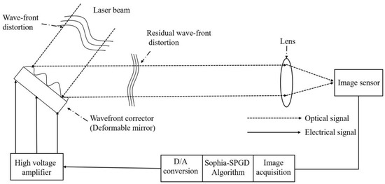
Figure 1.
Schematic of the WFS-less AO system. The solid lines indicate electrical signals, the dashed lines indicate optical signals, and the jagged lines indicate wavefront disturbances.
The distortion compensation process of the deformable mirror is achieved by altering the shape of its deformable surface to counteract the target wavefront distortions. There are many methods for representing the surface shape and wavefront; the most direct method is to represent the surface shape as , which is the distance of a point at coordinates from the horizontal plane. According to the working principle of the deformable mirror, the compensatory surface shape produced by the mirror can be represented by a linear combination of the influence functions of each actuator, and the equations are as follows:
Here, is the i-th control signal for the DM actuator, is the influence function of the i-th DM actuator, represents the coordinates on the wavefront plane, represents the coordinates of the i-th actuator on the DM, represents the spacing between adjacent elements, represents the coupling value between elements, and represents the Gaussian metric [13,14].
In the simulation experiment, a sum of 100 Kolmogorov phase screens under turbulence strengths of = 10, 15, and 20 are generated [28]. The phase screen comprises Zernike aberrations from the 3rd to the 104th order, excluding tilt terms. The statistical properties of the generated phase screen conform to the Kolmogorov spectrum, and the screens do not exhibit correlations between them. The turbulence intensity is denoted as , where is the telescope aperture and is the atmospheric coherence length. The optimization algorithm uses the mean radius (MR) and mean radius ratio (MRR) [29] as an optimization metric; the Strehl ratio (SR) [30] acts as an indicator metric. The MRR is the ratio between the average radius of the ideal far-field point spread function (PSF) and the average radius of the corrected PSF.
Allowing to be the phase distribution of the wave front, in a circular aperture, the complex amplitude of the wave front can be expressed as:
The relationship between the PSF and the complex amplitude of the wavefront can be described by means of Fourier transform. Performing a two-dimensional Fourier transform on the yields its representation of in the frequency domain, and the PSF can be obtained by calculating the square of the modulus of .
The formulas for the SR, mean radius ratio (MR), and MRR are given below:
where is the peak intensity of the image formed by the optical system with aberrations, is the peak intensity of the ideal diffraction-limited image, and MRideal is the ideal mean radius. The SRs are frequently used in numerical simulations as the system’s objective function because of their low computational demands and simple structure. SR values close to 1 indicate minimal aberration effects and a high image quality, whereas lower values suggest significant aberrations and a reduced image quality. The mean radius is an essential parameter for evaluating the quality of an optical system, as it measures the deviation of the actual wavefront from the ideal wavefront. A smaller mean radius signifies a closer approximation to the ideal, diffraction-limited wavefront, indicating a higher optical quality and enhanced imaging performance. Throughout the algorithm’s iterative process, MR values are recorded. For analytical convenience, changes in the SR values are also recorded alongside.
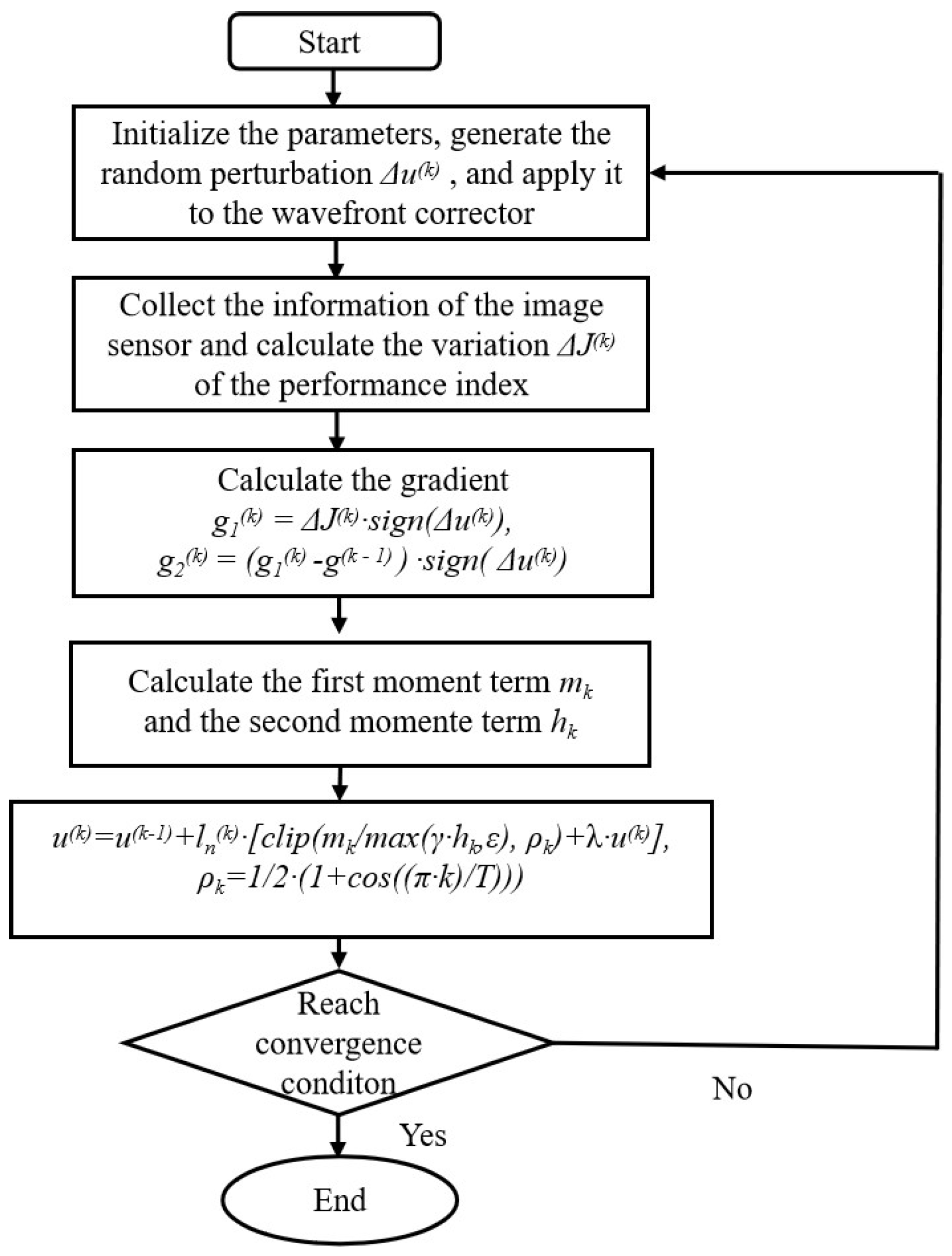
In this paper, we introduce a Sophia-optimized SPGD algorithm, referred to as Sophia-SPGD, which integrates the Sophia optimizer from deep learning with the traditional SPGD algorithm. The variation in the performance metrics of the spot image is approximated as a gradient. The algorithm incorporates momentum, adaptivity, and gradient clipping techniques in the gradient descent process. By utilizing the gradient momentum method, the algorithm compares the variation in gradients from the current and previous iterations. If the variation in gradients is in the same direction, it generates a positive excitation, whereas opposing directions cause a negative excitation. This method effectively minimizes oscillations throughout the iteration process, enhancing the stability and efficiency of the optimization. The learning rate is adaptively adjusted to mitigate local convergence issues. Additionally, the algorithm incorporates gradient clipping to control the step size of the gradient descent, ensuring that the performance indices of spot images do not fluctuate dramatically in the later stages of the iterations. This approach streamlines the optimization process, enhancing the efficiency and stability of wavefront corrections in WFS-less adaptive optics systems. The Sophia-SPGD algorithm flowchart is shown in Figure 2.
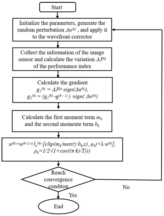
Figure 2.
Flowchart of the Sophia-SPGD algorithm.
The core concept of the stochastic parallel gradient descent (SPGD) algorithm involves estimating the gradient of control parameters through changes in performance metrics and randomized perturbation voltage vector . The algorithm iteratively searches for control voltage vectors along the direction of gradient descent until it finds a maximum value of the performance metrics. Here, the performance metric is a function of the control voltage vectors, expressed as , where represents the control voltages for the various units of the wavefront corrector.
The specific process is as follows: First, the system randomly generates a small perturbation voltage vector . Then, the positive perturbation voltages are applied to the DM to obtain the CCD images and calculate the positive performance metrics , and the negative perturbation voltages are applied to the DM via a similar method to obtain the negative performance metrics . The formula for calculating the variation in performance metrics is as follows:
where represents the gain coefficient, which is generally a positive value; is the voltage of the deformable mirror controller added during the k-th iteration; denotes the number of corrective units in the wavefront corrector; and is the randomly disturbed voltage vector applied during the k-th iteration. The control voltage vector is calculated in accordance with Formula (6) and applied to the deformable mirror. Images are collected to obtain the correction effect, and the k-th iteration is completed.
SPGD is pervasively recognized as an effective method for performance metric optimization; however, the use of a fixed gain coefficient limits its adaptability for wavefront correction in wavefront sensorless adaptive optics systems. This leads to suboptimal correction results, slow correction speeds, and an easy fall into the local optimum. To increase the convergence speed and reduce the probability of falling into the local optimum, the momentum of inertia and adaptive learning rates are the most common considerations.
In the Sophia-SPGD algorithm, the first-order gradient and the second-order gradient are calculated according to Equations (11) and (12):
where is the sign function, which determines the sign of a number. The sign of and its performance are determined by the direction of optimization of the performance metrics. If the performance metrics increase, takes a positive value; otherwise, it takes a negative value.
In the Sophia-SPGD algorithm, the introduction of a momentum term aims to accelerate learning and reduce oscillations. Here, represents the first-order momentum term, and represents the first-order momentum term. and are momentum hyperparameters, typically ranging between 0 and 1. The first-order momentum of the gradient and the second-order momentum of the gradient according to in Equations (13) and (14) are calculated as follows:
These formulas imply that the current momentum is a weighted average of the previous momentum and the current gradient. These two momentum terms play crucial roles in the parameter update process. By integrating past momentum with current gradient information, the algorithm progresses more steadily toward the optimal solution. This approach prevents overly sensitive parameter changes in situations of drastic gradient variations and enhances the convergence speed and robustness of the algorithm.
The primary role of adopting an adaptive learning rate is to balance the convergence speed and avoid becoming trapped in local optima during the optimization process. Adaptive-learning-rate algorithms automatically adjust the learning rate according to different parameters and formula conditions. In the initial stages of iteration, a higher learning rate is provided to accelerate convergence. As the iteration progresses and the performance indices gradually approach their extremum, the learning rate automatically decreases to prevent significant fluctuations near the optimal solution, thus ensuring stable convergence to the optimum. The relationship between the learning rate and the number of iterations is expressed as
Here, is a manually predefined initial learning rate. is the attenuation rate.
Introducing weight decay when updating control voltages can smooth the changes in parameter update, thereby accelerating the convergence speed. As discussed above, the Sophia-SPGD algorithm is used to update the control voltage vector computation formula as follows:
where represents the voltage signal for the iteration and where is the total number of iterations. The clipping function is used to limit within the range of the adaptive function , and is a very small constant set to 10−8 to avoid dividing by 0. In the above equation, the typical parameters are , , , , . Using an adaptive function to limit the range of the clipping function can effectively increase the convergence accuracy in the later stages of iteration and prevent falling into a local optimum.
The implementation of the Sophia-PGD algorithm is comprehensively described in Algorithm 1.
| Algorithm 1. Sophia-SPGD |
| Inputs: The learning rate , the initial learning rate , hyperparameters , , , , the constant , the initial momentum coefficient . Output: Calculated control voltage vectors 1: Set , where N is the number of corrector channels. Set , , . 2: for k = 1 to do 3: Randomly generate perturbed voltages 4: Compute the perturbation of performance indicators , , and 5: Compute 6: 7: 8: 9: |
| 10: |
| End |
To implement SPGD or any of its variants, a performance metric must be specified. Here, the MR and SR are used to measure the correction performance of the algorithm and are defined as shown in Equations (3) and (4). Through numerical simulation, we can further observe and assess the performance of the Sophia-SPGD algorithm in practical scenarios to determine its effectiveness and advantages in enhancing correction performance.
3. Simulations and Analysis
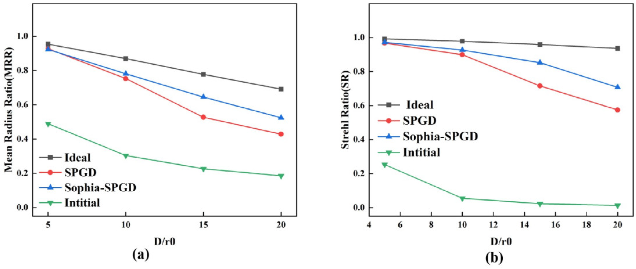
To analyze the feasibility of the Sophia-SPGD algorithm, we first select the optimal parameters for each algorithm on the basis of many simulation experiments under various turbulence intensities. Then, we use both algorithms to correct the same set of randomly generated wavefront aberrations and compare the simulation results. The number of correction iterations is set at 1500. A 97-element DM is introduced to perform the simulations. Figure 3 shows the obtained averaged SR and MRR adaptation curves. Except for cases with turbulence intensity , the correction capability of Sophia-SPGD surpasses that of SPGD, particularly in the presence of stronger turbulence.
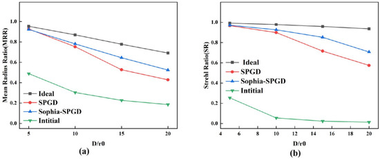
Figure 3.
Convergence extreme values of (a) MRR and (b) SR after 1500 iterations of Sophia-SPGD and traditional SPGD under turbulence strengths D/r0 = 5, 10, 15, and 20.
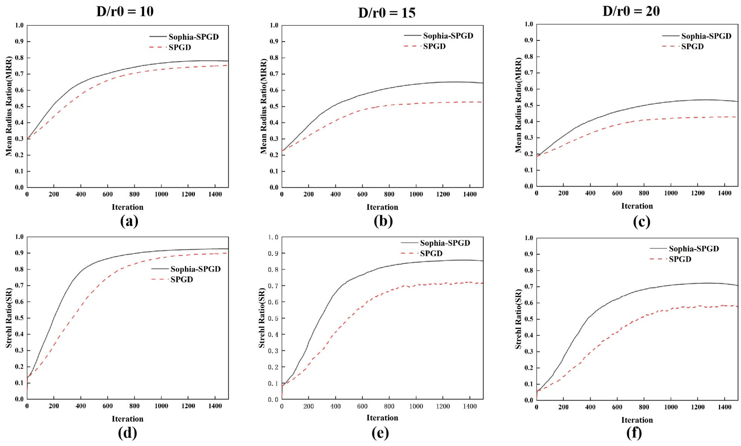
During the simulation process, 100 frames of random wavefront aberrations under different turbulence intensities of D/r0 = 10, 15, and 20 were used as correction subjects to analyze the convergence speeds of the Sophia algorithm and the SPGD control algorithms. The average correction results of the 100 frames of random aberrations serve as the experimental outcome, with each of the four algorithms iterating 1500 times. The average MRR and average SR adaptation curves are presented in Figure 4. Both the SPGD and Sophia-SPGD algorithms have sufficiently converged after 1500 iterations. Comparing the convergence curves of different algorithms under the same turbulence conditions, it is evident that at lower turbulence, Sophia does not demonstrate a significant advantage in terms of convergence speed over SPGD. However, a comparison of the convergence curves under varying turbulence conditions reveals that as the turbulence intensity increases, the convergence performance of the Sophia-SPGD control algorithm progressively exceeds that of the SPGD control algorithm. The Sophia-SPGD and SPGD algorithms can effectively optimize and compensate for aberrations to some extent. However, under high-turbulence conditions, the correction accuracy is degraded because of the limitations of the correction capacity of the deformable mirror.
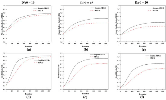
Figure 4.
Adaptive process of the adaptive optical system with D/r0 = 10, 15, and 20 when the Sophia-SPGD and SPGD control algorithms are used. (a–c) MRR curves; (d–f) the corresponding SR curves.
To observe the wavefront correction effects of the SPGD and Sophia-SPGD algorithms more objectively, a typical phase screen generated under a turbulence strength of D/r0 = 10 is selected. The uncorrected wavefront, its corresponding 3rd–18th Zernike coefficients and initial uncorrected PSF, are provided in Figure 5a, b, and c, respectively. The simulation results obtained via the SPGD algorithm are shown in Figure 5d–f, and the simulation results obtained via the Sophia-SPGD algorithm are shown in Figure 5h–i. After 500 iterations, both of the above algorithms eliminate the wavefront aberration effectively, and the corresponding far-field point spread function (PSF) takes shape well. Judging from the distribution of the Zernike coefficients corresponding to the wavefront residuals after correction by the two algorithms, the correction performance of the Sophia-SPGD algorithm is better than that of the SPGD algorithm.
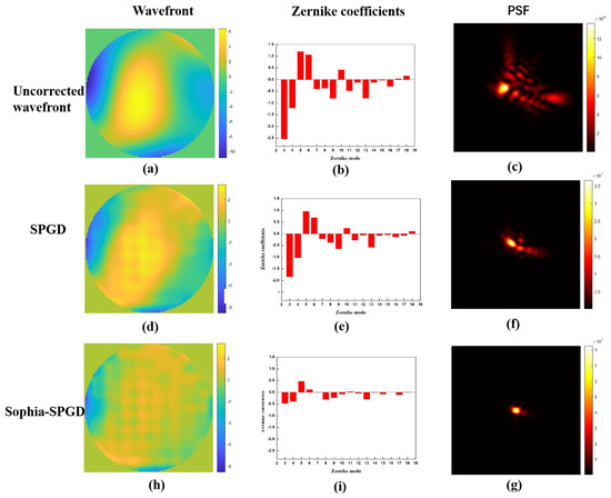
Figure 5.
Wavefront aberration correction and the corresponding far-field point spread function (PSF) of a typical phase screen generated under turbulence strength . The number of iterations is set to 500. (a) Uncorrected wavefront. (d) Wavefront corrected with SPGD. (h) Wavefront corrected with Sophia-SPGD. (b,e,i) The corresponding Zernike coefficients of wavefront. (c,f,g) The corresponding PSFs of wavefront, respectively.
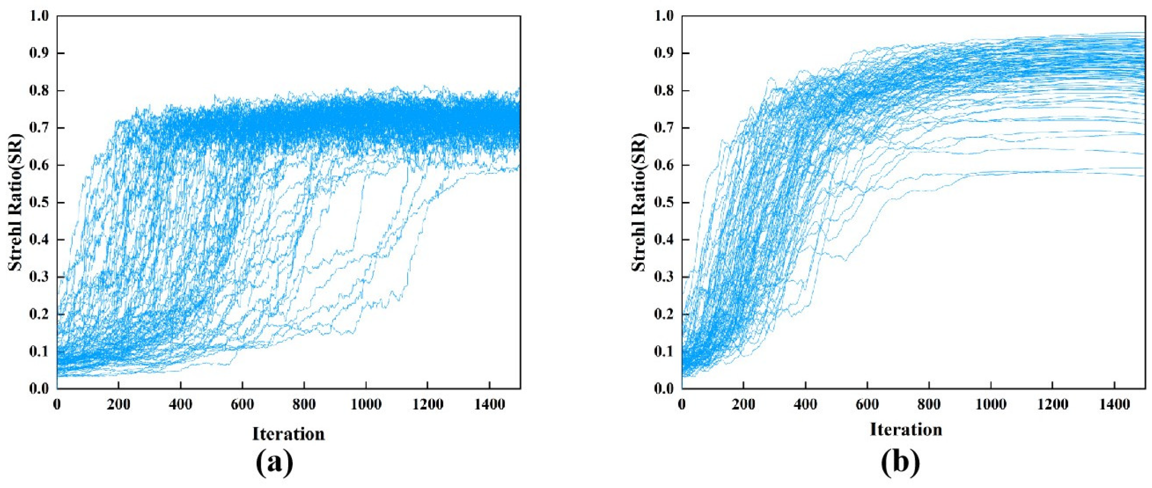
In order to investigate whether the algorithms fluctuate in the later iterations of the wavefront correction, we give the SR iteration curves of the SPGD and Sophia optimization algorithms, respectively (Figure 6). The atmospheric turbulence strength is D/r = 15 for all of these realizations. It is shown that, during the iteration, the SR curve of conventional SPGD exhibits fluctuations. In contrast, the SR curve of the Sophia-SPGD algorithm is relatively smooth during the iteration and shows no significant fluctuations in the later stage of the iteration.

Figure 6.
The SR curves of 100 realizations of (a) SPGD and (b) Sophia-SPGD under turbulence strength D/r0 = 15.
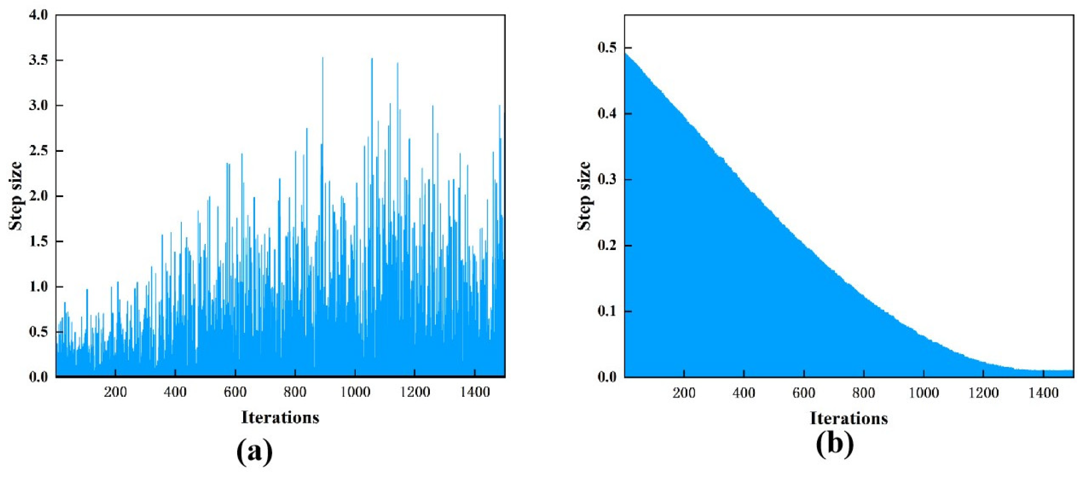
In addition, to better verify the stability of the algorithm, we use the Euclidean norm to measure the parameter update of the control voltage vector during the iteration. Figure 7 illustrates the in each step size of each algorithm throughout the iteration process. During the iteration of SPGD, the changes in adjacent step sizes are very drastic. In contrast, during the iteration of Sophia-SPGD, the changes in adjacent step sizes are gentle and tend to be stable in the later stage of the iteration.

Figure 7.
Step size of the k-th iteration during the whole iterative procedure of (a) SPGD and (b) Sophia-SPGD algorithms.
Convergence speed is a critical metric in the control of adaptive optics systems. Under three different conditions of strong turbulence, the initial average MR values were 0.304, 0.227, and 0.186, respectively; after correction by the SPGD control algorithm, the average MRR values at the convergence extremum were 0.753, 0.527, and 0.428, respectively. Calculating 80% of the MRR correction range under different turbulence conditions yielded values of 0.663, 0.467, and 0.380. These values serve as benchmarks to analyze and compare the number of iterations required by the two control algorithms to achieve the same correction effect, as shown in Table 1. The simulation data demonstrate that the Sophia algorithm is more efficient than the SPGD algorithm. At a turbulence strength of D/r0 = 10, the correction speed of the Sophia-SPGD algorithm is 35.6% faster than that of the SPGD algorithm; at D/r0 = 15, it is 75% faster; and at D/r0 = 20, it is 79.5% faster.

Table 1.
Comparison of the average value of the MRR and the number of times that 80% of the local optimum is reached between the two algorithms under different turbulence strengths.
Under three different conditions of strong turbulence, the initial average SR values were 0.136, 0.084, and 0.058; after correction by the SPGD control algorithm, the average MR values at the convergence extremum were 0.899, 0.714, and 0.575, respectively. Calculating 80% of the SR correction range under different turbulence conditions yielded values of 0.746, 0.573, and 0.472. These values serve as benchmarks to analyze and compare the number of iterations required by the two control algorithms to achieve the same correction effect, as shown in Table 2. At a turbulence strength of D/r0 = 10, Sophia-SPGD’s correction speed is 65.9% faster than that of SPGD; at D/r0 = 15, it is 80.4% faster; and at D/r0 = 20, it is 93.2% faster.
Table 2.
Comparison of the average value of the SR and the number of times that 80% of the local optimum is reached between the two algorithms under different turbulence strengths.
In conclusion, the convergence results from both the MR and SR indicate that as the turbulence intensity increases, the convergence effectiveness becomes constrained. Notably, under conditions of strong turbulence, Sophia-SPGD consistently achieves faster convergence than SPGD.
4. Experiments and Results
To evaluate the correction capability of the wavefront sensorless adaptive optics system based on the Sophia algorithm, the aberrations within the experimental system were selected as the reference aberrations. These aberrations were used to control a 97-element piezoelectric deformable mirror, and experiments were conducted to verify the correction performance for both point targets and extended targets. The deformable mirror used was a high-speed deformable mirror with 97 piezoelectric elements manufactured by ALPAO, France, with an effective aperture of 22.5 mm and an actuator spacing of 2.5 mm. The CCD camera utilized was the Prime BSI Express Scientific camera, which was developed and produced by Teledyne Photometrics. The experimental results were evaluated via the MR as a performance metric.
In the point target correction experiment, the experiment setup was carried out referring to the optical path shown in Figure 1. We employed an adjustable-power semiconductor laser (wavelength of 635 nm) as the light source. During the experiment, the laser emitted a 22.5 mm diameter beam through a collimating system, matching the effective aperture of the deformable mirror. The beam is reflected by an anamorphic mirror, passes through a beam reduction mirror (12.5×), and finally focuses on the target surface of the CCD camera through a focusing lens (f = 150 mm). An image acquisition card captured the speckle information detected by the CCD and transferred it to a MATLAB 2022b program on the computer for analysis. The program calculates the average radius of the speckles within a selected area as a performance metric for the algorithm. The required control voltages for the deformable mirror were converted by a D/A card, amplified by a high-voltage amplifier, and applied to 97 elements of the mirror, causing it to deform and optimize the speckle radius. The algorithm iterates until it reaches a predetermined number of iterations or converges to an optimal value. The algorithm used in this experiment was the same as that used in the previously described simulation experiment.
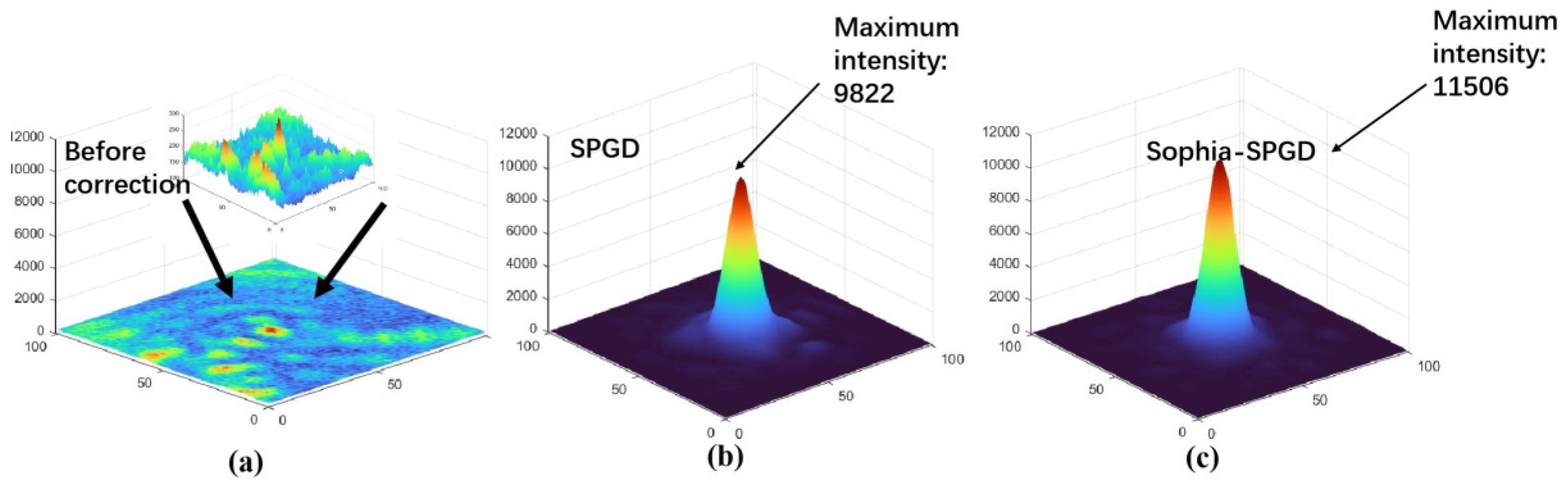
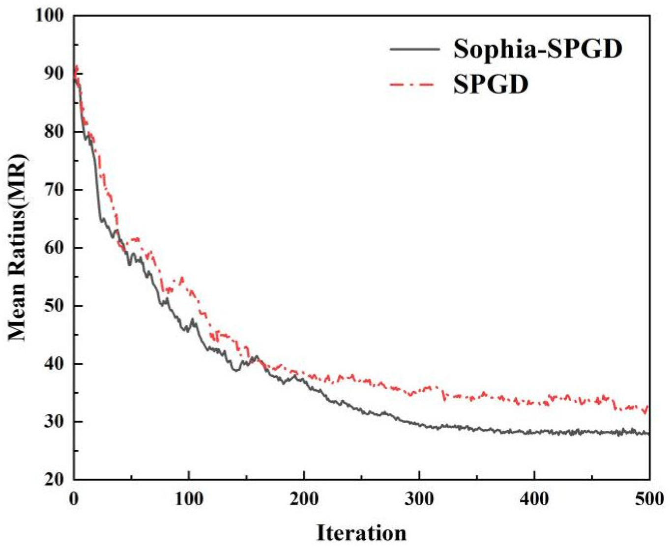
Figure 8a displays the far-field intensity distributions before correction under system static aberration. The diffraction limit of the experimental system used was calculated to be 19.8 pixels. Visually, the far-field speckle patterns reveal that the SPGD algorithm improved the MR from 89 pixels to 36 pixels, whereas the Sophia-SPGD algorithm increased it from 89 pixels to 27 pixels. Additionally, the number of iterations required to reach a far-field speckle size of three times the diffraction limit was 152 and 133 for the SPGD and Sophia-SPGD algorithms, respectively. Three-dimensional far-field intensity distributions are shown in Figure 8b,c, where it can be clearly seen that the largest value of central energy was obtained with the Sophia-SPGD-algorithm’s correction. Figure 9 shows the experimentally obtained MR curves during correction via the SPGD and Sophia-SPGD algorithms.
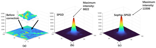
Figure 8.
Comparison of 3D far-field intensity distributions: (a) before correction under static aberration; (b,c) after correction with the SPGD and Sophia-SPGD algorithms.
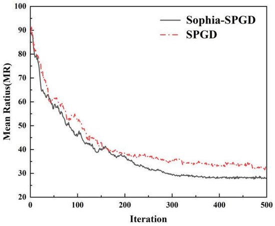
Figure 9.
MR curves for the SPGD and Sophia-SPGD algorithms.
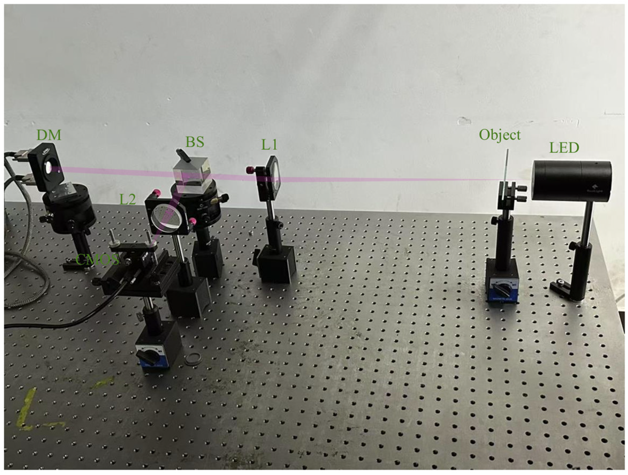
The extended-target-correction experimental system layout is shown in Figure 10. We used an LED with a center wavelength of 570 nm as the light source. The extended target was a resolution test board, model GH-YP832, Guangzhou, China which consisted of 29 sets of four-direction stripes with line widths from 2.5 µm to 500 μm. The diffraction limit of the constructed optical system was 25 µm. The anamorphic mirror was a 97-unit MEMS DM made by ALPAO, Grenoble, France, for aberration correction. The camera was a 16-bit CDD camera. Lens L1 has a focal length of 400 mm, and L2 has a focal length of 100 mm, both of which form a 4f system. This process is similar to point target tests: an image acquisition card collects information about the extended target from the CCD camera and transfers it to MATLAB 2022b programs on a computer for analysis. The program evaluates the algorithm’s performance via an image frequency evaluation function within a selected area. The control voltages for the deformable mirror, which are calculated via the algorithm, are converted and amplified before being applied to the 97 elements of the mirror, which induces deformation to optimize the performance metrics. The algorithm iterates until it reaches a predetermined number of iterations or converges to the optimal value. The algorithm used in this experiment was the same as that employed in previous simulation experiments.
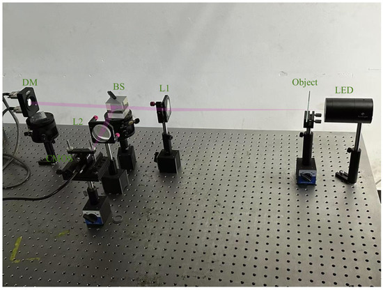
Figure 10.
Experimental system layout.
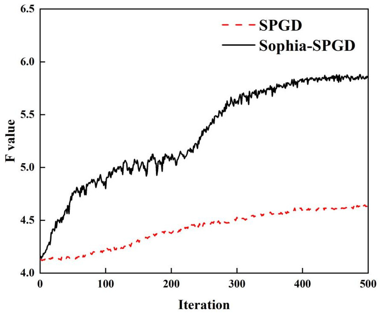
Figure 11a shows that the original stripe image is blurred in detail. After correction with the SPGD algorithm (Figure 11b), although there was some improvement in image detail, blurriness remained. Figure 11c shows that the newly proposed Sophia-SPGD algorithm successfully removed the blurred details, resulting in a clearer overall structure that more closely approximated the ideal diffraction-limited image. Image quality was assessed via the custom-modified frequency assessment function F. The F value of the image before correction was 4.1275; after correction, the F value of the SPGD algorithm was 4.6399; and the F value of the Sophia-SPGD algorithm was 5.8653.

Figure 11.
Reconstruction results of object imaging degraded by aberrations in the system. (a) Initial uncorrected image, (b) correction image via SPGD, (c) correction image via Sophia-SPGD.
F value curves after correction via the SPGD and Sophia-SPGD algorithms are shown in Figure 12. Compared with SPGD, Sophia-SPGD requires fewer iterations to achieve the same image quality evaluation metric. The images corrected by the SPGD algorithm were unsatisfactory, whereas the images corrected by Sophia-SPGD had satisfactory visual results.

Figure 12.
The F value curves for the SPGD and Sophia-SPGD algorithms.
5. Conclusions
This paper introduces an improved SPGD algorithm, termed Sophia-SPGD, aimed at addressing the poor adaptability of the gradient update within the algorithm, thereby enhancing the convergence speed and accuracy of the SPGD algorithm and reducing the likelihood of falling into local optima. The Sophia-SPGD algorithm approximates the minor changes in system performance indices as gradients, calculates the first and second moments of these gradients, and introduces mechanisms for weight decay and adaptive shearing limit updates. This allows for adaptive adjustment of the gain coefficient, improving the system’s convergence accuracy, accelerating the convergence speed, and reducing the probability of settling into local minima. Through numerical simulations and experiments, our algorithm was compared with the traditional SPGD algorithm. The results demonstrate superior performance under various atmospheric turbulence conditions compared with the SPGD algorithm. The Sophia-SPGD algorithm can reduce the number of iterations and the probability of falling into local optima. Moreover, the parameter adaptability of the Sophia-SPGD algorithm is stronger than that of the SPGD algorithm. Overall, the Sophia-SPGD algorithm proposed in this paper features a rapid convergence speed and is less prone to local optima, making it more promising for practical applications.
Author Contributions
Conceptualization, P.C. and H.Y.; methodology, P.C.; software, W.Y. and Z.Z.; validation, Y.G., X.L. and Z.Q.; resources, H.Y.; writing—original draft preparation, P.C.; writing—review and editing, H.Y.; funding acquisition, H.Y. All authors have read and agreed to the published version of the manuscript.
Funding
This research was funded by the National Laboratory on Adaptive Optics, China (grant number FNLAO-24-MS-O01); the National Natural Science Foundation of China (grant numbers 12473081 and U2141255); and the Jinling Institute of Science and Technology High-level Talent Introduction Program (grant number jit-b-201813).
Institutional Review Board Statement
Not applicable.
Informed Consent Statement
Not applicable.
Data Availability Statement
The data presented in this study are available on request from the corresponding author.
Conflicts of Interest
The authors declare no conflicts of interest.
References
- Tyson, R.K.; Frazier, B.W. Principles of Adaptive Optics; CRC Press: Boca Raton, FL, USA, 2022. [Google Scholar]
- Madec, P.Y. Overview of deformable mirror technologies for adaptive optics and astronomy. In Adaptive Optics Systems III; SPIE: Bellingham, WA, USA, 2012; Volume 8447, pp. 22–39. [Google Scholar]
- Martínez, N.; Ramos, L.F.R.; Sodnik, Z. Simulating the performance of adaptive optics techniques on FSO communications through the atmosphere. In Laser Communication and Propagation Through the Atmosphere and Oceans VI; SPIE: Bellingham, WA, USA, 2017; Volume 10408, pp. 49–57. [Google Scholar]
- Li, M.; Gao, W.; Cvijetic, M. Slant-path coherent free space optical communications over the maritime and terrestrial atmospheres with the use of adaptive optics for beam wavefront correction. Appl. Opt. 2017, 56, 284–297. [Google Scholar] [CrossRef] [PubMed]
- Primot, J. Theoretical description of Shack–Hartmann wave-front sensor. Opt. Commun. 2003, 222, 81–92. [Google Scholar] [CrossRef]
- Antonello, J.; van Werkhoven, T.; Verhaegen, M.; Truong, H.H.; Keller, C.U.; Gerritsen, H.C. Optimization-based wavefront sensorless adaptive optics for multiphoton microscopy. J. Opt. Soc. Am. A 2014, 31, 1337–1347. [Google Scholar] [CrossRef] [PubMed]
- Yang, H.; Soloviev, O.; Verhaegen, M. Model-based wavefront sensorless adaptive optics system for large aberrations and extended objects. Opt. Express 2015, 23, 24587–24601. [Google Scholar] [CrossRef]
- Zhang, Y.; Zhang, H.; Yuan, G. A Phase Recovery Technique Using the Genetic Algorithm for Aberration Correction in a Coherent Imaging System. Sensors 2023, 23, 7679. [Google Scholar] [CrossRef]
- Yang, P.; Hu, S.J.; Chen, S.Q.; Yang, W.; Xu, B.; Jiang, W.H. Research on the phase aberration correction with a deformable mirror controlled by a genetic algorithm. In Journal of Physics: Conference Series, International Symposium on Instrumentation Science and Technology, 8–12 August 2006, Harbin, China; IOP Publishing: Bristol, UK, 2006; Volume 48, No. 1. [Google Scholar]
- Yue, W.; Jin, G.; Yang, X. Adaptive Particle Swarm Optimization for Automatic Design of Common Aperture Optical System. Photonics 2022, 9, 807. [Google Scholar] [CrossRef]
- Hu, X.; Yang, D.; Dou, J.; Yang, Z.; Liu, Z. Differential evolution algorithm-based aberration correction method for the interference of vortex beams. Appl. Phys. B Laser Opt. 2022, 128, 133. [Google Scholar] [CrossRef]
- Li, Z.; Cao, J.; Zhao, X.; Liu, W. Atmospheric compensation in free space optical communication with simulated annealing algorithm. Opt. Commun. 2015, 338, 11–21. [Google Scholar] [CrossRef]
- Yang, H.; Zang, X.; Zhang, Z.; Liu, J. Wavefront Correction System Based on RUN Optimization Algorithm. Acta Photonica Sin. 2023, 52, 1111004. [Google Scholar]
- Yang, H.; Zang, X.; Chen, P.; Hu, X.; Miao, Y.; Yan, Z.; Zhang, Z. An Efficient Method for Wavefront Aberration Correction Based on the RUN Optimizer. Photonics 2024, 11, 29. [Google Scholar] [CrossRef]
- Vorontsov, M.A.; Sivokon, V.P. Stochastic parallel-gradient-descent technique for high-resolution wave-front phase-distortion correction. J. Opt. Soc. Am. A 1998, 15, 2745–2758. [Google Scholar]
- Zhao, H.; Lv, D.; An, J.; Kuang, K.; Yu, M.; Zhang, T. Meta-heuristic SPGD algorithm in spatial light wavefront distortion correction. Infrared Laser Eng. 2022, 51, 20210759. [Google Scholar]
- Li, J.; Wen, L.; Liu, H.; Wei, G.; Cheng, X.; Li, Q.; Ran, B. A Novel SPGD Algorithm for Wavefront Sensorless Adaptive Optics System. IEEE Photonics J. 2023, 15, 7801109. [Google Scholar]
- Zhao, H.; An, J.; Yu, M.; Lv, D.; Kuang, K.; Zhang, T. Nesterov-accelerated adaptive momentum estimation-based wavefront distortion correction algorithm. Appl. Opt. 2021, 60, 7177–7185. [Google Scholar] [PubMed]
- Zhang, H.; Xu, L.; Guo, Y.; Cao, J.; Liu, W.; Yang, L. Application of AdamSPGD algorithm to sensor-less adaptive optics in coherent free-space optical communication system. Opt. Express 2022, 30, 7477–7490. [Google Scholar]
- Song, H.; Fraanje, R.; Schitter, G.; Kroese, H.; Vdovin, G.; Verhaegen, M. Model-based aberration correction in a closed-loop wavefront-sensor-less adaptive optics system. Opt. Express 2010, 18, 24070–24084. [Google Scholar]
- Dong, B.; Li, Y.; Han, X.-L.; Hu, B. Dynamic Aberration Correction for Conformal Window of High-Speed Aircraft Using Optimized Model-Based Wavefront Sensorless Adaptive Optics. Sensors 2016, 16, 1414. [Google Scholar] [CrossRef]
- Verstraete, H.R.G.W.; Wahls, S.; Kalkman, J.; Verhaegen, M. Model-based sensor-less wavefront aberration correction in optical coherence tomography. Opt. Lett. 2015, 40, 5722–5725. [Google Scholar] [CrossRef]
- Yang, G.; Liu, L.; Jiang, Z.; Guo, J.; Wang, T. Incoherent beam combining based on the momentum SPGD algorithm. Opt. Laser Technol. 2018, 101, 372–378. [Google Scholar]
- Song, J.; Li, Y.; Che, D.; Wang, T. Numerical and experimental study on coherent beam combining using an improved stochastic parallel gradient descent algorithm. Laser Phys. 2020, 30, 085102. [Google Scholar]
- Fang, Z.; Xu, X.; Li, X.; Yang, H.; Gong, C. SPGD algorithm optimization based on Adam optimizer. In AOPC 2020: Optical Sensing and Imaging Technology; Luo, X., Jiang, Y., Lu, J., Liu, D., Eds.; International Society for Optics and Photonics, SPIE: Bellingham, WA, USA, 2020; Volume 11567, p. 115672S. [Google Scholar]
- Xu, L.; Wang, J.; Yang, L.; Zhang, H. Design and Performance Analysis of NadamSPGD Algorithm for Sensor-Less Adaptive Optics in Coherent FSOC Systems. Photonics 2022, 9, 77. [Google Scholar] [CrossRef]
- Liu, H.; Li, Z.; Hall, D.; Liang, P.; Ma, T. Sophia: A scalable stochastic second-order optimizer for language model pretraining. arXiv 2023, arXiv:2305.14342. [Google Scholar]
- Assémat, F.; Wilson, R.W.; Gendron, E. Method for simulating infinitely long and non stationary phase screens with optimized memory storage. Opt. Express 2006, 14, 988–999. [Google Scholar] [PubMed]
- Jiang, P.; Liang, Y.; Xu, J.; Mao, H. A new performance metric on sensorless adaptive optics imaging system. Optik 2016, 127, 222–226. [Google Scholar]
- Bobroff, N.; Rosenbluth, A.E. Evaluation of highly corrected optics by measurement of the Strehl ratio. Appl. Opt. 1992, 31, 1523–1536. [Google Scholar]


Disclaimer/Publisher’s Note: The statements, opinions and data contained in all publications are solely those of the individual author(s) and contributor(s) and not of MDPI and/or the editor(s). MDPI and/or the editor(s) disclaim responsibility for any injury to people or property resulting from any ideas, methods, instructions or products referred to in the content. |
© 2025 by the authors. Licensee MDPI, Basel, Switzerland. This article is an open access article distributed under the terms and conditions of the Creative Commons Attribution (CC BY) license (https://creativecommons.org/licenses/by/4.0/).