Pilot-Assisted Phase Recovery in Coherent Optical Receivers with Robust Locally Weighted Interpolation

Abstract

Accurate and low-complexity phase estimation is crucial for optimal data recovery in coherent optical receivers, especially for applications in emerging scenarios such as low-margin optical networks, green networks, probabilistic-shaping modulation, the use of high-order modulation formats in hollow-core fibers, long-haul links operating at low signal-to-noise ratios, and free-space optical links in low-earth orbit satellites, among others. These new developments demand highly efficient and reliable data transmission methods, even under stringent conditions of minimal operational excess margin. This paper introduces an efficient pilot-assisted phase estimation strategy for coherent optical receivers, integrating robust interpolation techniques for quasi-optimal operation. Our approach significantly enhances phase estimation accuracy, addressing the unique challenges posed by these new scenarios. Through comprehensive simulations, we illustrate our method’s superiority over conventional methods, showcasing marked improvements in computational complexity and bit error rate. The results highlight the critical role of sophisticated interpolation in bolstering pilot-assisted phase estimation, offering a promising technique for optimizing performance in next-generation coherent optical receivers.

1. Introduction

In high-bandwidth networks, coherent optical communication systems play a crucial role in addressing the ever-growing demand for data transmission capacity. However, these systems face significant challenges, particularly in managing phase noise that affects coherent receivers. Pilot-assisted techniques for tracking phase noise in optical systems may be essential in current low-margin optical network scenarios, where maintaining signal integrity is crucial. Despite notable progress in developing robust compensation techniques, as highlighted in [1,2], phase noise remains a substantial barrier, especially as data rates and modulation complexities increase.

The minimum distance estimator (MDE), for instance, has demonstrated superior capabilities in tracking phase noise across various quadrature amplitude modulation (QAM) formats. However, its complexity increases with the modulation order, requiring a larger number of trial phases and longer filter lengths for denser constellations, thereby imposing heavier computational burdens. This increase in processing may affect communication latency. Optimizing resource efficiency is crucial, particularly for high-order modulation schemes that are resource intensive. In green optical networks, for example, power management, especially through power scaling and adaptive modulation, is vital. Therefore, exploring alternative strategies or innovative combinations of the MDE and other phase-tracking methods is essential.

In the design of low-margin optical networks, the system margin (S-margin) accounts for time-varying network conditions, including slow-varying impairments due to network aging. This aging process can cause laser de-tuning, leading to misalignment with optical filters in intermediate nodes, such as reconfigurable optical add-drop multiplexers (ROADMs). Typically, transponder aging introduces a margin of $0.5\mathrm{dB}$ [3]. These mismatches in local oscillator lasers can affect the laser linewidth, which directly increases phase noise, negatively impacting overall system performance. Advancements in this field aim to achieve an optimal balance between improving system performance and reducing resource consumption, thereby ensuring the scalability and reliability of future optical communication networks.

Recent studies have emphasized the potential of pilot-aided carrier phase recovery (PA-CPR) as a promising approach to address phase random-walk challenges in coherent optical receivers [4,5,6,7,8,9]. The effectiveness of PA-CPR in mitigating phase noise is particularly noteworthy, as pilot symbols experience the same phase perturbations as data symbols, providing a reliable reference for phase correction. Typically, these pilot symbols are high-energy, known deterministic symbols such as binary phase shift keying (BPSK) or quadrature phase shift keying (QPSK), with well-defined phase angles, enabling accurate phase estimation. This approach can facilitate the development of new algorithms for low-margin network systems.

The adoption of new technologies, such as hollow core fibers (HCFs), has expanded to various applications, including low-latency transmission, data centers, radio front-haul, and experimental data transmission using coherent and direct detection transceivers [10]. These advances present significant opportunities for dense wavelength division multiplexing (DWDM) networks in the coming years. HCFs offer substantial advantages over traditional single-mode fibers (SMFs) and photonic shield core fibers (PSCFs), such as extremely low optical nonlinearity (over 1000 times weaker than SMFs), higher optical power handling, longer repeater spacing, reduced attenuation, new low-loss transmission bands, and low chromatic dispersion, making them highly suitable for very-high-order modulation formats. Consequently, phase estimation algorithms for these technologies should be able to efficiently operate up to 256QAM and higher-order modulation formats.

The low latency of nested antiresonant nodeless fibers (NANFs) is particularly advantageous, primarily due to their effective refractive index, $n_{\mathrm{eff}}\approx 1$. However, several challenges must be addressed, such as the inability to perform Raman amplification within the transmission fiber, difficulties in interconnecting the SMF to the HCF or the HCF to the HCF, and fiber leakage issues, particularly in extreme environments such as deep-sea applications or highly urbanized areas exposed to extreme heat. HCFs also have a more rigid core structure compared to traditional solid core fibers, making them less flexible and more prone to microbending losses. This rigidity complicates installation and handling, especially in environments that require tight bends or complex routing. Furthermore, their delicate microstructured design makes HCFs more difficult to manipulate, splice, and terminate, requiring specialized equipment and techniques to minimize losses and maintain performance [11].

In latency-sensitive applications such as telemedicine or high-frequency trading [12], $n_{\mathrm{eff}}$ is not the only critical parameter. Beyond short-distance transmissions, where accumulated loss and dispersion (including chromatic dispersion and polarization mode dispersion) are within acceptable limits, it becomes crucial to employ streamlined transponders that minimize time-consuming signal processing tasks, such as forward error correction (FEC), dispersion compensation, and complex coding/decoding in modulation. Therefore, novel techniques are needed to ensure that the latency gains achieved with HCFs are not negated by processing overhead [11].

The use of burst pilots can significantly simplify the coding and decoding processes in modulation while maintaining the low-latency advantages of hybrid coding frameworks by reducing the signal processing burden. A key benefit of pilot symbol-based systems is their inherent reconfigurability, which enables seamless adaptation to various modulation formats. This flexibility is particularly valuable for phase recovery algorithms (e.g., MDE), which require modulation-specific adjustments. Additionally, an inherent advantage of using pilots is that they eliminate the need for differential encoding.

In practical systems, differential encoding is often employed to address phase ambiguity, particularly when the absolute phase of the signal is unknown. However, its associated penalties must be carefully considered. Theoretical penalties for differential encoding have been calculated as 3 dB, 2.22 dB, 1.55 dB, and 1.04 dB for QPSK, 16QAM, 64QAM, and 256QAM, respectively [13].

In the blind phase search (BPS) algorithm, differential encoding plays a critical role in resolving phase ambiguities that arise during phase estimation. BPS estimates the phase with potential ambiguities in multiples of ${\displaystyle \frac{2\pi }{M}}$ for MQAM signals. The penalties for differential encoding in the BPS algorithm are reported as 0.7 dB, 0.6 dB, 0.5 dB, and 0.5 dB for QPSK, 16QAM, 64QAM, and 256QAM, respectively [1]. Similarly, [14] reports penalties of 0.5 dB and 0.4 dB on a receiver BER of ${10}^{-3}$ for set-partitioning 128 polarization-multiplexed 16QAM (128-SP-QAM) and polarization-multiplexed 16QAM (PM-16QAM), respectively.

The study in [15] investigates the impact of differential encoding on higher-order modulation formats and phase recovery. The authors highlight that differential coding is often employed to address cyclic phase slipping problems. However, they note that differential encoding and decoding introduce an approximately 1 dB penalty in optical signal-to-noise ratio (OSNR) sensitivity, especially when combined with high-coding-gain FEC. To overcome this limitation, the study proposes a training-assisted two-stage phase recovery algorithm, which eliminates the need for differential encoding. This approach reduces the OSNR penalty by about 1 dB and enhances the receiver sensitivity.

The work in [16] explores the benefits of a pilot-aided approach to mitigate cycle slips. Specifically, it reports OSNR gains of approximately 3.1 dB, 1.3 dB, and 0.6 dB (pre-FEC) for a 56 Gbit/s QPSK signal using a Viterbi–Viterbi (VV) algorithm cascaded with a pilot-aided phase-unwrapping (PAPU) technique. These gains were achieved with filter lengths of 8, 16, and 20, respectively, at a pre-FEC BER of $1.8\times {10}^{-2}$. Furthermore, the study claims post-FEC OSNR gains of 3 dB, 1 dB, and 0.5 dB under similar conditions.

The ability to dynamically adapt modulation formats to network traffic conditions is crucial for optimizing energy efficiency, enabling significant energy savings in optical networks. The modulation format switch has shown the potential to reduce energy consumption by as much as 18% [17]. Green optical networks are essential for meeting the growing demands of artificial intelligence (AI), which requires substantial computational resources and data transfer. Using advanced optical technologies to minimize power consumption, these networks support AI scalability while maintaining sustainability, a vital balance as AI and environmental concerns converge. Likewise, coherent communications are being considered for short-range applications to meet the growing demand for bandwidth [18].

In addition to HCFs, free-space optical (FSO) links in low-earth orbit (LEO) satellites represent another critical technology driving 6G wireless communications. However, this technology imposes much stricter pointing requirements and is highly susceptible to atmospheric turbulence and the demanding precision needed for optical beam alignment. Coherent communications maximize system capacity by leveraging the advantages of coherent modulation in both amplitude and phase, directly connecting optical systems without electronic conversion, reducing processing requirements and leading to energy savings [19,20].

Designing low-complexity carrier recovery algorithms for coherent FSO links remains a significant challenge. The Viterbi–Viterbi (VV) algorithm [21,22], designed specifically for phase shift keying (PSK) modulation, exploits the constant amplitude and uniform phase transitions of PSK signals. It employs a 4th-power operation to remove modulation and recover the carrier’s frequency and phase. However, this power operation significantly amplifies the background noise in the received signal. To mitigate this, a low-complexity joint compensation scheme for carrier recovery (JCSCR) has been proposed [23], which relies on the addition and subtraction of real absolute values based on modulated phase information, effectively avoiding the noise-enhancing 4th-power operation used in the VV algorithm for coherent FSO communications. In addition, other implementations utilize pilot-based channel estimation, bridging the gap between coherent fiber optic communications and free-space optical systems [24].

As discussed previously, these methods are inherently modulation dependent. For higher-order modulation formats, pilot-aided carrier phase recovery (PA-CPR) provides a modulation-format-independent approach to phase noise compensation. Moreover, PA-CPR exhibits significantly lower computational complexity compared to maximum likelihood (ML)-based detection and estimation algorithms, making it a more practical choice for high-speed optical communication systems.

A key advantage of PA-CPR is its ability to continuously track laser phase noise over the full phase range of 0 to $2\pi$, thereby enabling the use of absolute phase information for data transmission. This capability eliminates the optical signal-to-noise ratio (OSNR) penalties typically associated with differential coding, leading to improved system performance [5].

However, the effectiveness of PA-CPR strongly depends on the design of the pilot symbol, particularly the pilot spacing. Rapid fluctuations in laser phase noise impose a fundamental limit on the temporal effectiveness of pilot-based estimation, restricting its accuracy to short time intervals, as noted in [25]. Optimizing pilot placement and density is therefore crucial for maintaining robust phase noise compensation in practical implementations.

To address the ever-increasing demand for capacity, recent research has explored the use of probabilistic shaping to increase the Euclidean distance between constellation points and enhance digital signal processing (DSP) algorithms [26]. A promising approach combines probabilistic shaping with extended Kalman filtering [27]. Specifically, a rate-adaptive coded modulation scheme with probabilistic signaling has been integrated with the BPS algorithm [28] in order to reduce overhead while optimizing system performance.

Previous studies have explored methods for correcting phase cycle slips by integrating coarse phase detection with interpolators, along with the use of a maximum likelihood (ML) algorithm to correct residual phase offsets [29]. Additionally, advancements in FEC techniques have enabled the reduction of required pre-FEC signal-to-noise ratio (SNR) values, allowing signals to be recovered at lower SNR levels. These developments require more robust phase recovery and improved performance in challenging communication environments.

In this study, we present the implementation of pilot-aided carrier phase recovery (PA-CPR) in a burst-mode configuration, where pilot symbols are inserted into every L consecutive symbol. To optimize efficiency, the burst length was set at $L=32$, limiting the overhead to approximately $3\%$ of the total number of symbols. Initially, a linear regression interpolation (LRI) method was used for carrier phase recovery. This approach was chosen over frequency filter-based interpolation to avoid dependence on the entire signal for phase tracking. To further enhance performance, the LRI method was improved by integrating a hard-decision filter. This filter uses a noise variance threshold to identify and eliminate outliers, significantly improving accuracy compared to the standalone LRI method. We then explore an advanced technique to refine and stabilize phase tracking. Although smooth fitting curves have been a staple in signal processing for decades [30,31], our novel approach incorporates a cosine filter to remove outliers, followed by a localized weighted smoothing technique to improve phase tracking accuracy. This approach achieves significant computational efficiency by using pilot symbols for phase tracking. Using only the information between the pilot symbols in a burst mode, we eliminate the need to process the entire signal for phase interpolation, resulting in substantial computational savings.

The structure of this paper is organized as follows. Section 2 describes the system model, providing a detailed explanation of the PA-CPR technique, the LRI model, and the locally weighted regression (LWR) method. In addition, relevant pseudocodes are included to facilitate the replication of the proposed algorithms. Section 3 presents the simulation setup and results, offering a comparative analysis of the various methods studied. Section 4 analyzes the computational complexity of the cosine-robust locally weighted scatterplot smoothing algorithm (Cosine-RLOWESS) compared to the BPS method and the run-time comparison. In Section 5, the results of our research are further examined by comparing the performance of pilot-based techniques and evaluating their computational complexity. Finally, Section 6 summarizes the key findings and conclusions of this work.

2. System Model

In this section, we present the model for implementing pilot sequences and outline the methodology for simulating phase noise using a random-walk process. We then describe the application of linear regression to perform linear interpolation. In addition, we explore advanced techniques for outlier elimination, focusing on cosine filtering in conjunction with robust local weighting methods for smoothing. These techniques play a crucial role in reducing the impact of noise-induced distortions. In general, this discussion provides a comprehensive understanding of the key steps required for effective phase recovery in the implementation of pilot sequences.

2.1. Model System Setup

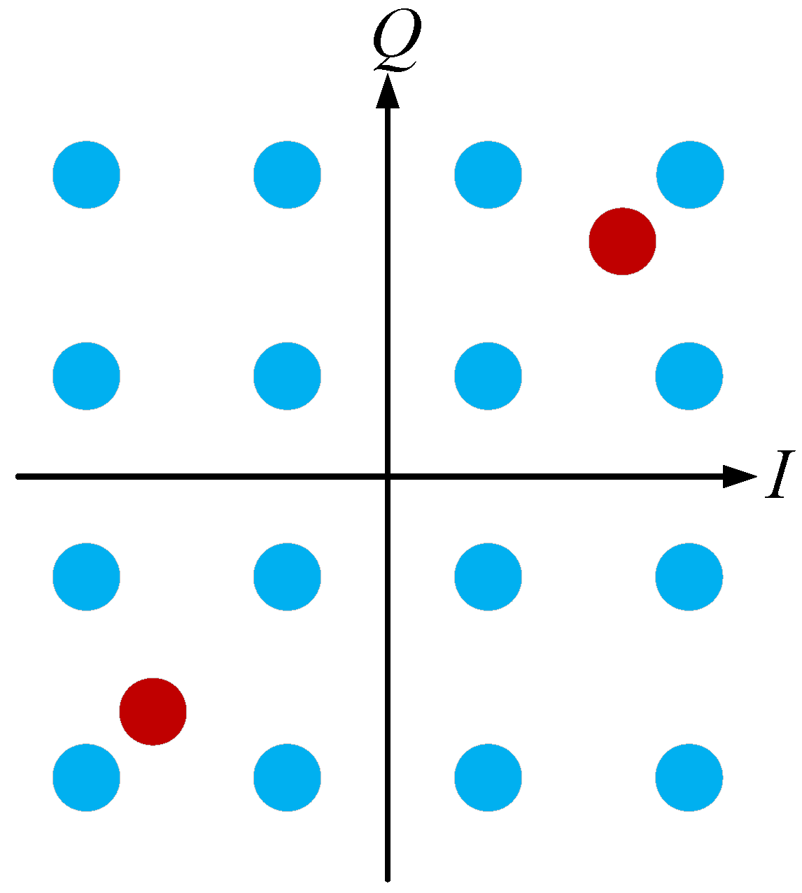
In our model, we implement the periodic insertion of pilot signals using BPSK modulation with a rotation of $\pi /4\mathrm{rad}$. This rotation helps to differentiate pilot signals from the square modulation used in data transmission. For the transmitter, we used square modulation schemes set through QPSK, 16QAM, 64QAM, and 256QAM constellations. An example of the model transmitting pilots can be seen in Figure 1 for a 16QAM modulation.

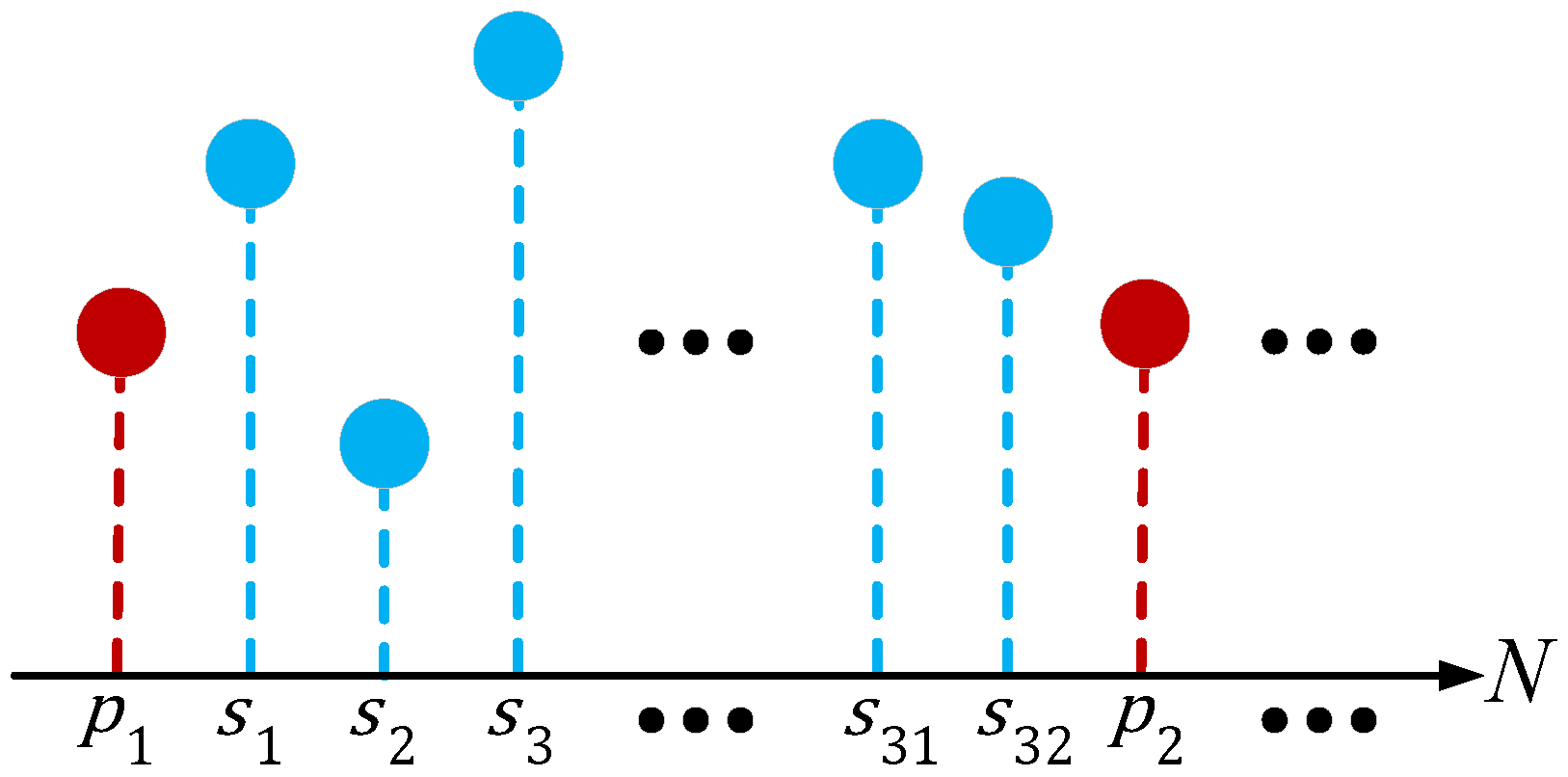
The pilot symbols were periodically inserted into the transmitted signal, following every 32 randomly generated data symbols. In the following discussion, we demonstrate that this interval can be adjusted. These pilot symbols serve as reference points, enabling the interpolator to accurately track and recover the phase, even in the presence of phase noise. Figure 2 illustrates an example of the transmitted symbols and pilots: the red markers indicate the pilot symbols, while the blue markers represent the data symbols generated by the modulator prior to transmission through the channel.

Consider the nth constellation symbol, $x\left[n\right]$, which is transmitted over a complex additive white Gaussian noise (AWGN) channel, where it is subject to additive noise $\eta \left[n\right]$, which models the amplified spontaneous emission (ASE) noise generated from inline amplifiers. Additionally, phase noise, resulting from the frequency and phase offset between the transmitter and local oscillator lasers, is modeled as a multiplicative factor $e^{j\theta \left[n\right]}$. Consequently, the received symbol $y\left[n\right]$ is expressed as:

$$\begin{array}{c}\hfill y\left[n\right]=x\left[n\right]e^{j\theta \left[n\right]}+\eta \left[n\right],\end{array}$$

(1)

where $\eta \left[n\right]$ is a Gaussian noise characterized by a zero mean AWGN with variance ${\sigma }^2\left[n\right]$, generated by optical amplification [32]. In optical coherent systems, phase noise is primarily influenced by the linewidths of local oscillators and manifests itself as a random-walk process. This behavior is also affected by the SNR in the receiver [33]. Assuming an initial condition $\theta \left(0\right)=0$ at time $t=0$, the phase evolves over time and deviates from 0 due to the random-walk process. At any subsequent time $t=\Delta t$, the phase difference measured during the symbol period $T_S$ follows a Gaussian distribution, with its variance directly proportional to the line width $\Delta \nu$ [34], as follows:

$$\begin{array}{c}\hfill E\left[{(\theta (t=0)-\theta (t=\Delta t))}^2\right]=2\pi \Delta \nu \Delta t.\end{array}$$

(2)

The phase noise at time t can be modeled as a Wiener process [1], as follows:

$$\begin{array}{c}\hfill \theta \left(t\right)=\sum _{n=-\infty }^{t}w\left[n\right],\end{array}$$

(3)

where $w\left[n\right]$ is a random $\mathcal{N}(0,2\pi \Delta \nu T_S)$ Gaussian variable with zero mean and variance given by [32]:

$$\begin{array}{c}\hfill {\sigma }_w^2=2\pi \Delta \nu T_S.\end{array}$$

(4)

In our model, $T_S$ denotes the symbol period, while $\Delta \nu$ represents the combined linewidth of the transmitter laser and the local oscillator (LO). The phase difference between two adjacent symbols follows a zero-mean Gaussian distribution with a variance given in Equation (4).

Following the analytical and geometrical arguments in [27,35], the phase noise evolution is then described with good approximation as:

$$\phi \left[n\right]=\phi [n-1]+w\left[n\right].$$

(5)

2.2. Linear Interpolation for CPR

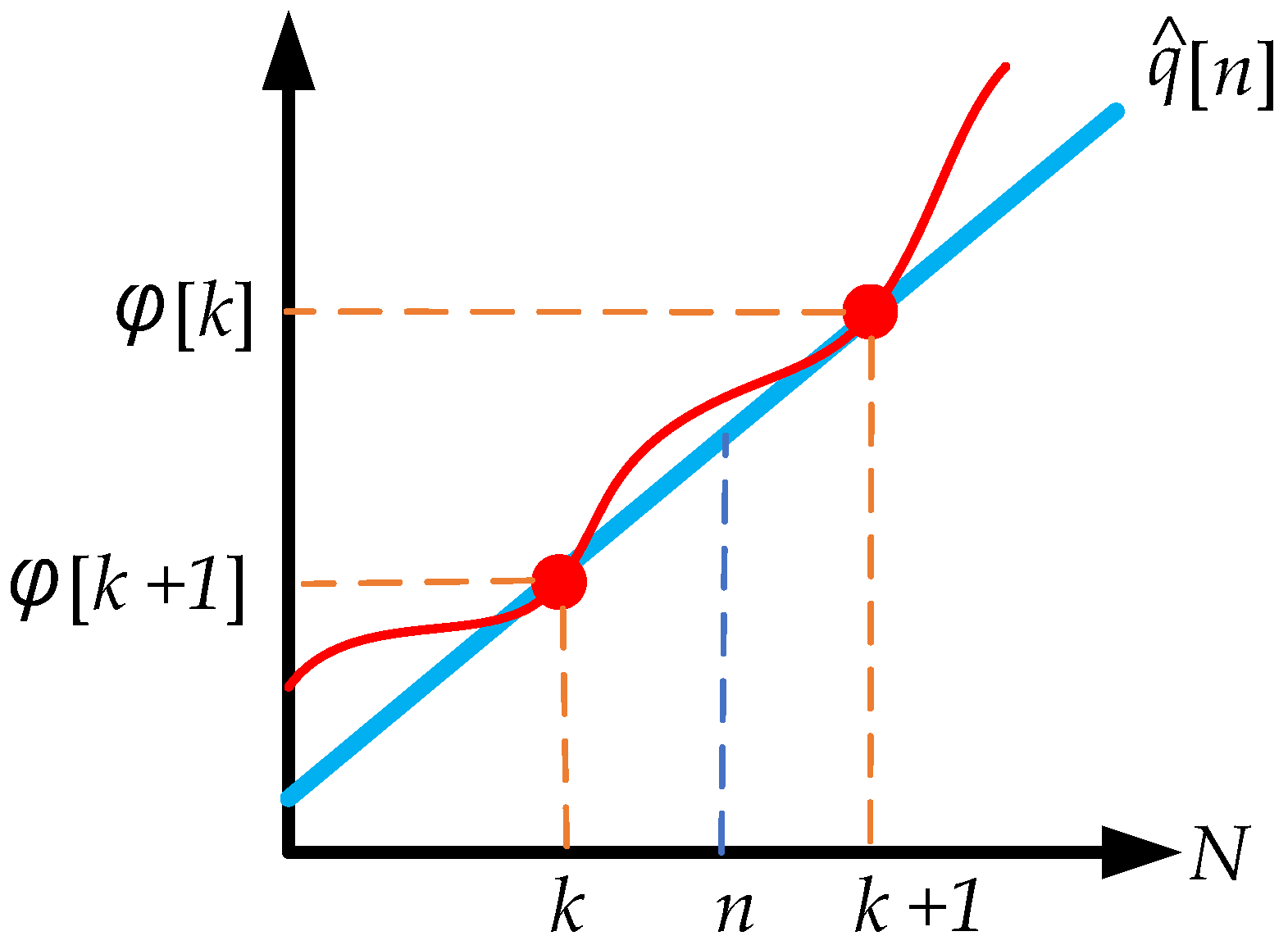
Linear interpolation is a straightforward regression method that is often used as a reference point in research. It serves as the foundation for experiments aimed at mitigating the impact of outliers that degrade phase recovery. The process begins by computing the coarse phase between consecutive pilot positions using the argument of the product between the received signal $y\left[n\right]$, at pilot positions $k=nL$, where $k=0,L,\dots ,K$, and the conjugate of the corresponding pilot sequence, $p\left[k\right]$.

The pilot sequence is introduced using the $\pi /4$-rotated BPSK modulation, as previously described, where k denotes the pilot positions. Specifically, the estimated phase at each pilot position is given by:

$$\begin{array}{c}\hfill \phi \left[k\right]=arg\left(y\left[Lk\right]p{\left[k\right]}^{*}\right),\end{array}$$

(6)

where ${[·]}^{*}$ denotes the conjugate operator and $\phi \left[k\right]$ represents the coarse phase in the pilot position, with pilots spaced in every $L=32$ samples. This burst length can be modified according to the resource conditions. The estimated phase, $\phi \left[k\right]$, can be used directly for linear interpolation, eliminating the need for a hard-decision filter. However, this approach may lead to degraded performance under certain conditions. In linear interpolation, it is assumed that the estimated phase $\hat{q}\left[n\right]$ is on the straight line connecting the nearest pilot phases $p\left[k\right]$ and $p[k+1]$, as illustrated in Figure 3.

The linear interpolated value $\hat{q}\left[n\right]$ is given by [36]:

$$\begin{array}{c}\hfill \hat{q}\left[n\right]=\phi \left[k\right]+\left({\displaystyle \frac{\phi [k+1]-\phi \left[k\right]}{L}}\right)\left([n-Lk]\right),\forall Lk<n\le L(k+1).\end{array}$$

(7)

In Algorithm 1, $\phi \left[k\right]$ denotes the value of the coarse phase at the pilot position, and n represents the position of the received symbols. Modification of linear interpolation using a hard-decision filter involves the use of a threshold ${\phi }_{th}$, which is estimated as ${\phi }_{th}=\pi {\sigma }_l$, where ${\sigma }_l$ represents the standard deviation of phase noise. The calculation of ${\sigma }_l$ is based on the burst length plus one $(L+1)$ and the noise variance ${\sigma }_w^2$ of the random phase, and is given by:

$$\begin{array}{c}\hfill {\sigma }_l=\sqrt{(L+1){\sigma }_w^2}.\end{array}$$

(8)

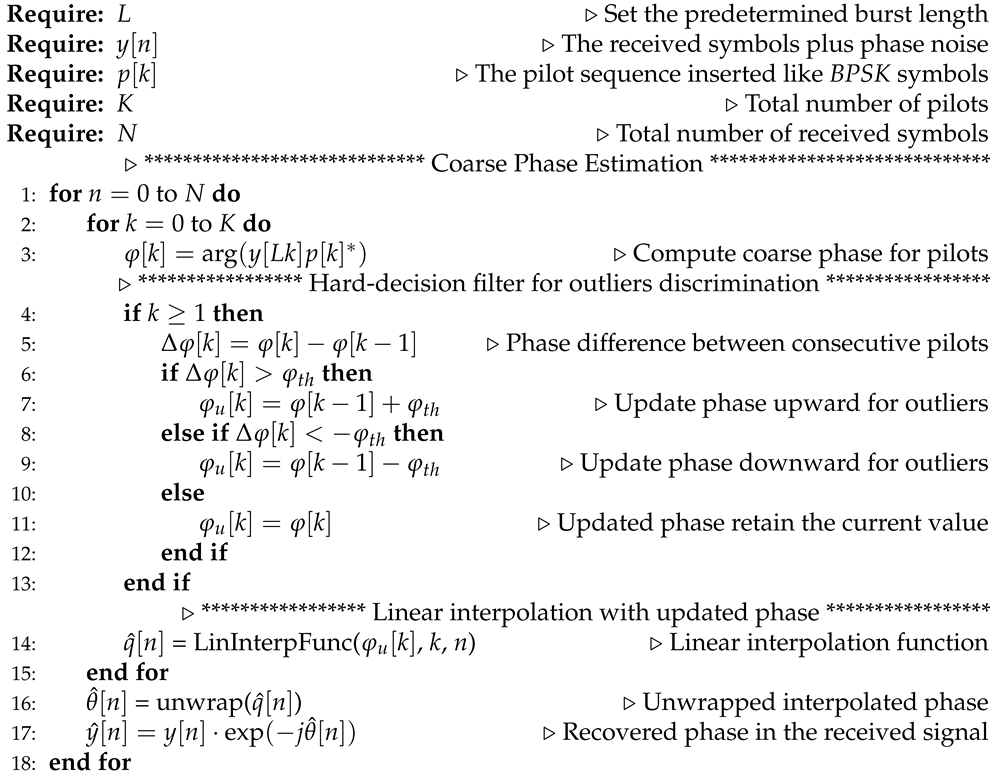
Algorithm 1 Hard-Decision Filter (HDF) Method for Outlier Detection and Linear Interpolation

A discrimination filter, which functions as a hard-decision filter, is applied prior to linear interpolation. This filter operates by limiting abrupt phase changes through a hard-decision approach based on the phase difference between consecutive pilots. The phase variation between consecutive pilots is defined as:

$$\begin{array}{c}\hfill \Delta \phi \left[k\right]=\phi \left[k\right]-\phi [k-1].\end{array}$$

(9)

For each pilot in the sequence, starting from the second pilot, i.e., $k=1,2,\dots ,K$, the updated phase value ${\phi }_u\left[k\right]$, after applying the hard-decision filter, is given by:

$$\begin{array}{c}\hfill {\phi }_u\left[k\right]=\left\{\begin{array}{cc}\phi [k-1]+\pi {\sigma }_l,\hfill & \mathrm{if}\Delta \phi \left[k\right]>\pi {\sigma }_l,\hfill \\ \phi [k-1]-\pi {\sigma }_l,\hfill & \mathrm{if}\Delta \phi \left[k\right]<-\pi {\sigma }_l,\hfill \\ \phi \left[k\right],\hfill & \mathrm{otherwise}.\hfill \end{array}\right.\end{array}$$

(10)

The updated phase at the pilot positions is then applied to a linear function to recover the phase signal.

The outlier discrimination process, implemented using a hard-decision filter, also described in Algorithm 1, detects deviations by analyzing the standard deviation of phase noise within the pilot sequence. This improves the precision of the phase estimation. When outliers fall outside a predefined critical range, the algorithm adjusts the phase at the pilot positions, either increasing or decreasing it to a more appropriate amplitude. If no outliers are detected, the current phase remains unchanged. The effectiveness of this method is illustrated in Section 3, with results highlighting its ability to track phase noise and its impact on BER performance.

2.3. Robust Locally Weighted Regression

The robust locally weighted regression method efficiently smooths the received symbols using a burst-based approach, excluding the necessity to process the entire signal or substantial segments of it. This method preferentially assigns greater weights to input symbols characterized by lower phase noise variance, thus reducing the impact of symbols affected by higher phase noise.

The robust method effectively identifies and eliminates outliers, mitigating distortions in the smoothed data points. This approach employs an iterative reweighting of the least-squares method [30,37]. A notable improvement in the algorithm’s performance is achieved by replacing the previously discussed hard-decision filter with a soft-decision filter that uses a cosine function for outlier discrimination. This enhanced filter incorporates information from both pilot symbols and data symbols interspersed between pilots.

The design of the soft-decision filter resulted from extensive experimental studies, which initially evaluated a Gaussian filter response. However, testing revealed that the cosine-based filter produced the most accurate results. This soft filter applies cosine-based corrections to severe outliers, ensuring smoother phase adjustments. Furthermore, the burst length is determined solely by the size of the pilot block, eliminating the need to rely on the entire signal or a large portion of it to correct the phase.

Unlike the hard-decision filter, the standard deviation ${\sigma }_w$ is directly derived from the phase noise and does not depend on the total length of the pilot sequence. Instead, it is calculated on the basis of the burst length, which corresponds to the interval between pilot samples. The parameter $\phi$ represents the coarse phase estimate. The equation for detecting and adjusting potential outliers at pilot positions, where $n=k$ indicates the pilot indices, is given by:

$$\begin{array}{c}\hfill w_f\left[n\right]=\left\{\begin{array}{cc}{\displaystyle \frac{1}{2}\left[1+cos\left(\frac{\pi {\sigma }_w}{2(Lk+k)}\right)\right]\phi [Lk+k],}\hfill & \mathrm{if}n=Lk,\hfill \\ {\displaystyle \frac{\beta }{2}\left[1+cos\left(\frac{\pi {\sigma }_w}{2(n+k)}\right)\right]\phi [n+k],}\hfill & \mathrm{if}n\ne Lk,\hfill \end{array}\right.\end{array}$$

(11)

in which $w_f\left[n\right]$ represents weights derived from a cosine function, with a default burst length of L. This length can be adjusted on the basis of the proportion of pilot symbols or the percentage of resources allocated to phase recovery, providing flexibility in configuration. These weights are applied to update the local weights of the process during the a-posteriori step. In Equation (11), $n\ne Lk$ specifies the indices of symbols located between the pilots. The parameter $\beta$ is a weighting factor chosen within the range $[0.65,0.95]$, experimentally determined as a function of the degradation of the phase noise $\Delta \nu T_S$. Outliers, identified as values that exceed twice the standard deviation of phase noise $(\phi >2{\sigma }_w)$, are set to zero to minimize their influence on phase tracking. The pseudocode for the enhanced algorithm is presented in Algorithm 2, where outliers are identified and mitigated using the modified cosine weighting function and then applied to the smoothing function.

After applying the soft-decision cosine filter for outlier discrimination, the robust locally weighted regression algorithm is applied. The received signal $y\left[n\right]$ is processed to obtain the coarse phase at the pilot positions and between the pilots using the burst division. The coarse phase $\phi \left[n\right]$ is divided into bursts of L samples each. The b-th burst, denoted as ${\phi }_b\left[n\right]$, can be expressed as:

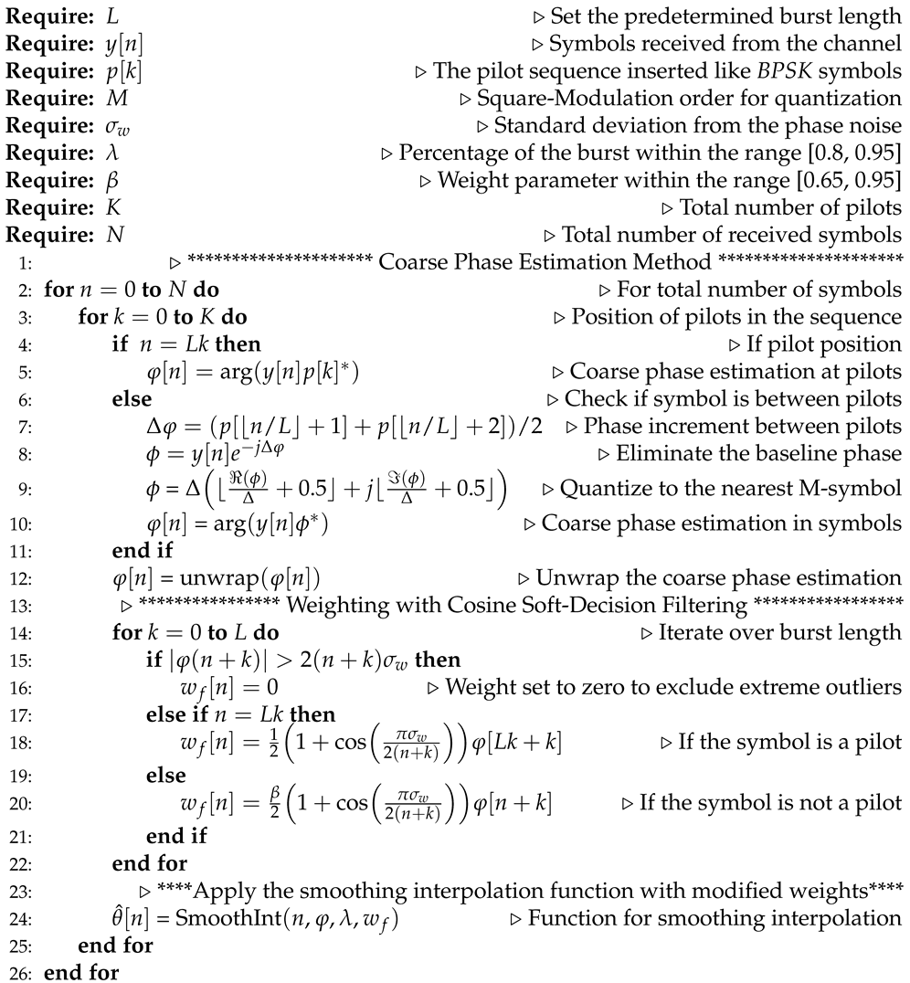
Algorithm 2 Enhanced Cosine Filter Method for Outlier Detection

$$\begin{array}{c}\hfill {\phi }_b\left[n\right]=\phi \left[n\right],n\in \{kL,kL+1,\dots ,kL+L-1\},\end{array}$$

(12)

where $k=0,1,2,\dots ,K$.

The locally weighted regression algorithm is used to calculate the fitted phase values based on the input coarse phase within the burst division ${\phi }_b\left[n\right]$. The signal $q\left[n\right]={\phi }_b\left[n\right]$ represents the phase to be processed. Accordingly, the equation representing the input to the algorithm for the smoothing process is given by:

$$\begin{array}{c}\hfill q\left[n\right]=g\left[n\right]+ϵ\left[n\right],\forall kL\le n<kL+L,0\le k<K.\end{array}$$

(13)

in which g denotes a smooth function. Instead of processing the entire signal at once, the algorithm operates on smaller fragments of the burst segment. The range specified in Equation (12) defines the windowed segment within the burst length across the entire signal. The noise term $ϵ\left[n\right]$ added in Equation (13) represents the residual phase noise; as the coarse phase $q\left[n\right]$ has not undergone any processing, it is the coarse phase received in burst mode. This noise is assumed to follow a normal distribution. The smoothed phase value at n, denoted by $\hat{q}\left[n\right]$, is obtained after applying the smoothing process.

The weight function $W\left[n\right]$ is adjusted based on the non-negative index n, increasing or decreasing accordingly. The weights $w_{\ell }\left[n\right]$ decrease as the distance between $n_{\ell }$ and n increases. The weights $w_{\ell }\left[n\right]$ are assigned to each burst, considering the neighboring symbols $-n_{\ell }\le \ell \le n_{\ell }$ and $\ell \ne 0$. This process centers the weight matrix W at n within the burst and scales it so that W becomes zero at the r-th nearest neighbor of n. The fitted value $\hat{q}\left[n\right]$ for each n is obtained by fitting a polynomial of degree d to the data using weighted least squares, with weights $w_{\ell }\left[n\right]$. This yields the initial set of fitted values. The residuals $\delta \left[n\right]$ are then computed as

$$\begin{array}{c}\hfill \delta \left[n\right]=q\left[n\right]-\hat{q}\left[n\right].\end{array}$$

(14)

In this framework, larger residuals result in smaller weights, while smaller residuals result in larger weights. This weighting process can be adjusted by manually assigning values at the pilot positions, where the information is theoretically more reliable. Consequently, the weights at the first and last positions of the burst, corresponding to known reference points, can be assigned to higher values. The methodology above is reapplied iteratively to update the fitted values using recalculated weights based on $\delta \left[n\right]$, continuously refining both the weights and the fitted values to achieve an improved fit.

The smoothing process g is designed to generate a robust approximation of $\hat{q}\left[n\right]$ by using neighboring points around n. The span, which defines the percentage of neighboring points that contribute to $\hat{q}\left[n\right]$, typically ranges from $10\%$ to $80\%$. In the absence of specific guidance for selecting the span, a default value of $50\%$ is often used. In Algorithm 2, the span is governed by the parameter $\lambda$, restricted within the range $[0.65,0.95]$.

The procedure for computing the robust weighting is as follows: Let $h\left[n\right]$ denote the distance from n to its r-th nearest neighbor. Specifically, $h\left[n\right]$ is the r-th smallest distance among $|n-\ell |$ and $\ell \ne n$. Then,

$$\begin{array}{c}\hfill w_{\ell }\left[n\right]=W\left(h{\left[n\right]}^{-1}|n-\ell |\right).\end{array}$$

(15)

Locally weighted regression (LWR) and robust locally weighted regression (RLWR) are characterized by the following sequence of operations:

• For each n, compute the estimates ${\hat{\beta }}_j\left[n\right]$ for $j=0,\dots ,d$, representing the parameters of a polynomial regression of degree d fitted to the data $(\ell ,q[n+\ell \left]\right)$. This regression is performed using weighted least squares, with weights $w_{\ell }\left[n\right]$ for each data pair $(\ell ,q[n+\ell \left]\right)$. The estimates ${\hat{\beta }}_j\left[n\right]$ are the values that minimize the following objective function:

  $$\sum _{\ell }{w}_{\ell }\left[n\right]{\left(q[n+\ell ]-{\beta }_0-{\beta }_1\ell -\dots -{\beta }_d{\ell }^d\right)}^2.$$

  (16)
  The smoothed point at n using a locally weighted polynomial regression of degree d is $(n,\hat{q}\left[n\right])$, where $\hat{q}\left[n\right]$ represents the fitted value of the regression at n. Thus,

  $$\hat{q}\left[n\right]=\sum _{j=0}^d{\hat{\beta }}_j{n}^{j+1}.$$

  (17)
• Define the bisquare weight function B as follows:

  $$B\left[n\right]=\left\{\begin{array}{cc}(1-n^2),\hfill & \mathrm{for}\left|n\right|<1,\hfill \\ 0,\hfill & \mathrm{for}\left|n\right|\ge 1.\hfill \end{array}\right.$$

  (18)
  Define the residuals based on the current fitted values as follows:
   

  $$e\left[n\right]=q\left[n\right]-\hat{q}\left[n\right].$$

  (19)
  Let s represent the median of the absolute residuals, $\left|e\right[n\left]\right|$. The robustness weights are then defined as follows:

  $$\delta [n+\ell ]=B\left({\displaystyle \frac{e[n+\ell ]}{6s}}\right).$$

  (20)
• For each n, compute the new $q\left[n\right]$ by fitting a polynomial of degree d using weighted least squares, where the weights for each pair $(\ell ,q[\ell \left]\right)$ are given by $\delta [\ell ]w_{\ell }\left[n\right]$.
• Repeat steps 2 and 3 for a total of ℓ iterations to obtain the final robust locally weighted regression fit values $\hat{q}\left[n\right]$. The weight function W is defined as a “tri-cube” function:

  $$W\left[n\right]=\left\{\begin{array}{cc}{(1-|n|}^3{)}^{(3/2)},\hfill & \mathrm{for}\left|n\right|<1,\hfill \\ 0,\hfill & \mathrm{for}\left|n\right|\ge 1.\hfill \end{array}\right.$$

  (21)

The pseudocode for carrier phase recovery by the LWR method is detailed in Algorithm 3 (the symbol ∘ represents element-wise power (Hadamard power), and the symbol ⊙ represents the Hadamard product, which involves multiplying corresponding elements of two vectors or matrices), while the computation for robust smoothing weighting is delineated in Algorithm 4.

Algorithm 3 Phase Computation Using the LOWESS Method

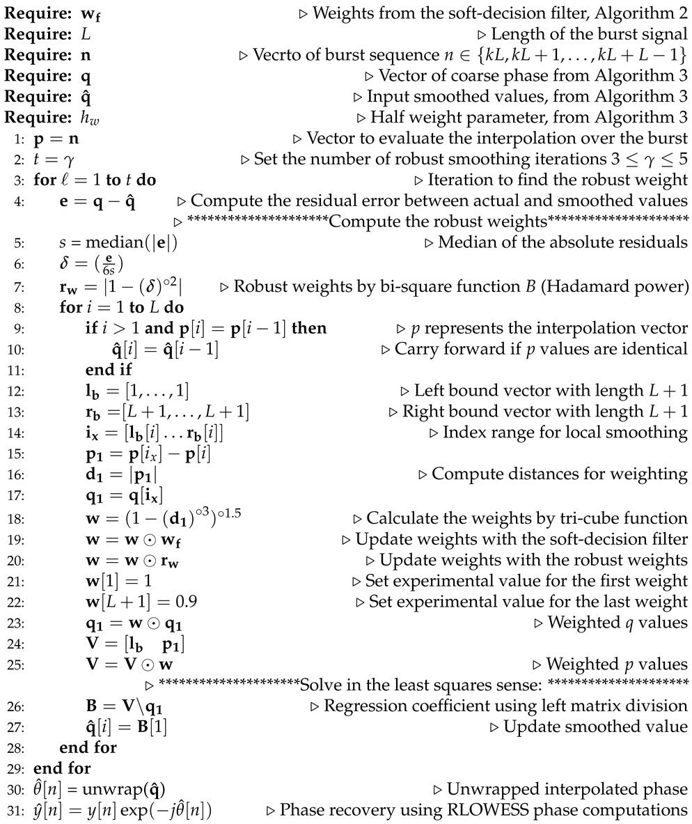
Algorithm 4 Robust Weight Computation for Fine Phase Recovery

A more detailed explanation of the robust locally weighted regression is available in [31]. One of the adaptations implemented in Algorithm 4 leverages the well-known positions of the pilots. Consequently, the data input is transmitted in burst mode, which means that the first and last symbols in the burst are always pilots. This setup allows for experimental data modifications at these two critical positions, depending on the quantity of phase noise or the modulation order.

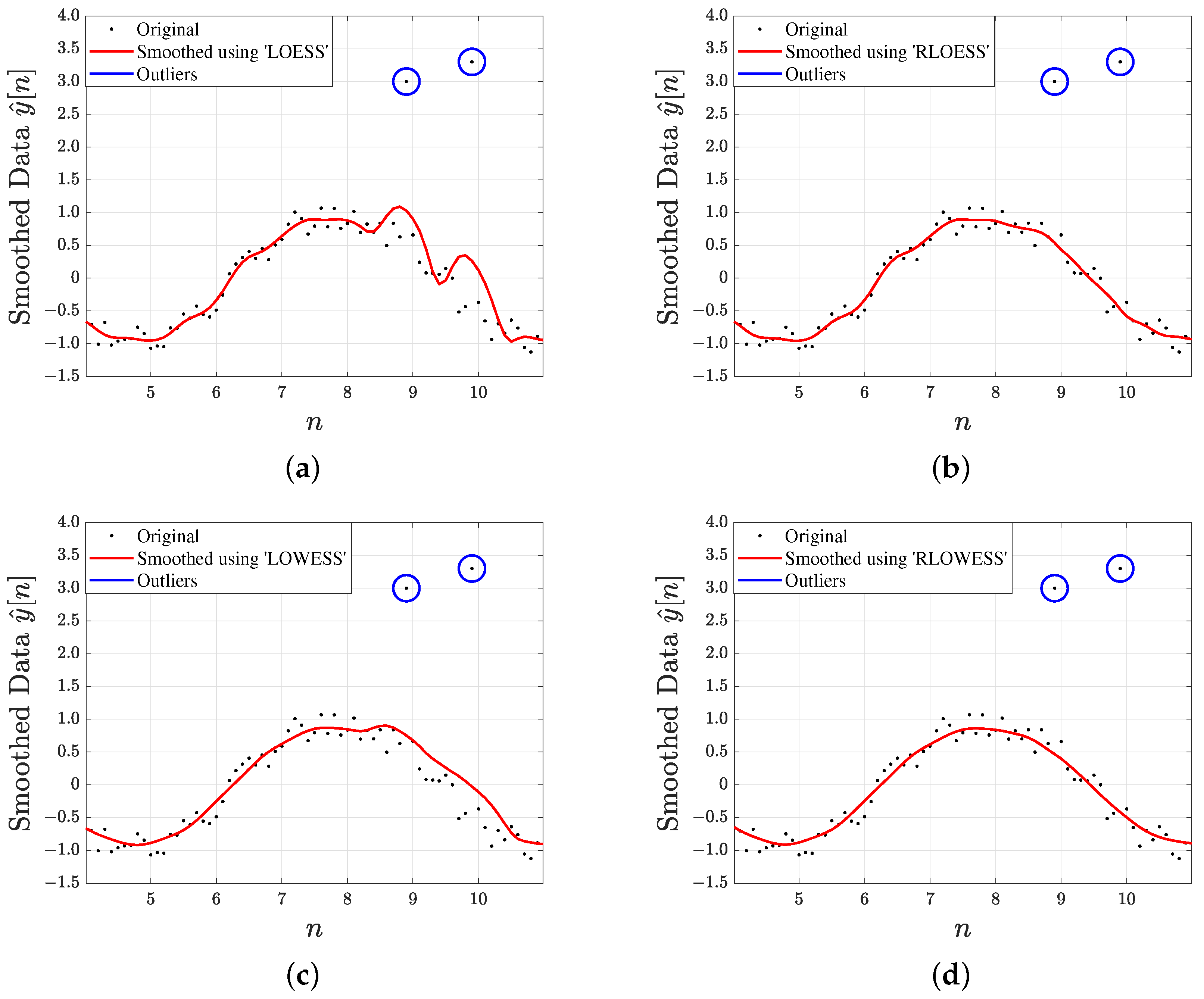
In Figure 4, we compare the performance of locally estimated scatterplot smoothing (LOESS), robust locally estimated scatterplot smoothing (RLOESS), locally weighted scatterplot smoothing (LOWESS), and robust locally weighted scatterplot smoothing (RLOWESS) in a simulation that includes specific outliers. Observations from Figure 4b,d indicate that both RLOESS and RLOWESS exhibit superior performance by effectively mitigating the influence of outliers.

The RLOESS method performs effectively on its own. Since it does not employ a weighted function, it is likely to have a lower computational cost and run faster than RLOWESS. However, the robust weighting approach in RLOWESS provides a key advantage: It allows weights to adapt dynamically, thereby reducing the impact of outliers. In addition, this adaptive weighting enhances flexibility, helps minimize the effects of phase noise, and facilitates the integration of the computed weights from the cosine filter.

3. Simulation Results

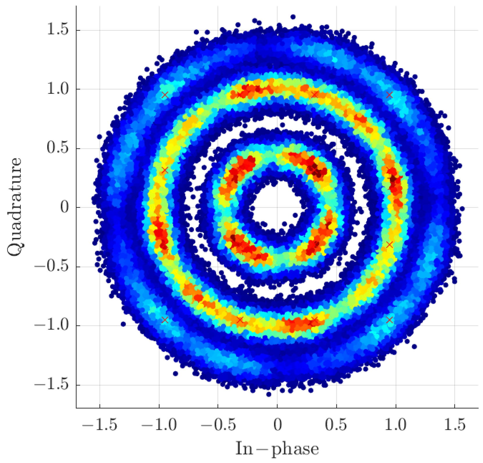
In this section, we analyze the simulations generated in our study. Figure 5 presents the constellation results for 16QAM with phase rotation. Furthermore, we applied our analysis to other modulation schemes, including QPSK, 64QAM, and 256QAM. For this experiment, phase noise was defined as $\Delta \nu =100\mathrm{kHz}\times 2$, accounting for contributions from both the transmitter and the receiver. A linewidth of $100\mathrm{kHz}$ is commonly used as a benchmark in phase compensation studies and is considered low enough that phase-locked loop (PLL) techniques become ineffective [1]. To achieve lower laser linewidths, below $100\mathrm{kHz}$, external cavity lasers (ECLs) are often employed. These devices are typically compact and suitable for small form factor transceivers and modules [38]. Therefore, instead of using PLL techniques, a feedforward carrier recovery method is recommended. The power level was set high, with $\mathrm{SNR}=20\mathrm{dB}$, to produce a cleaner constellation where the rotation effect due to phase noise is clearly visible.

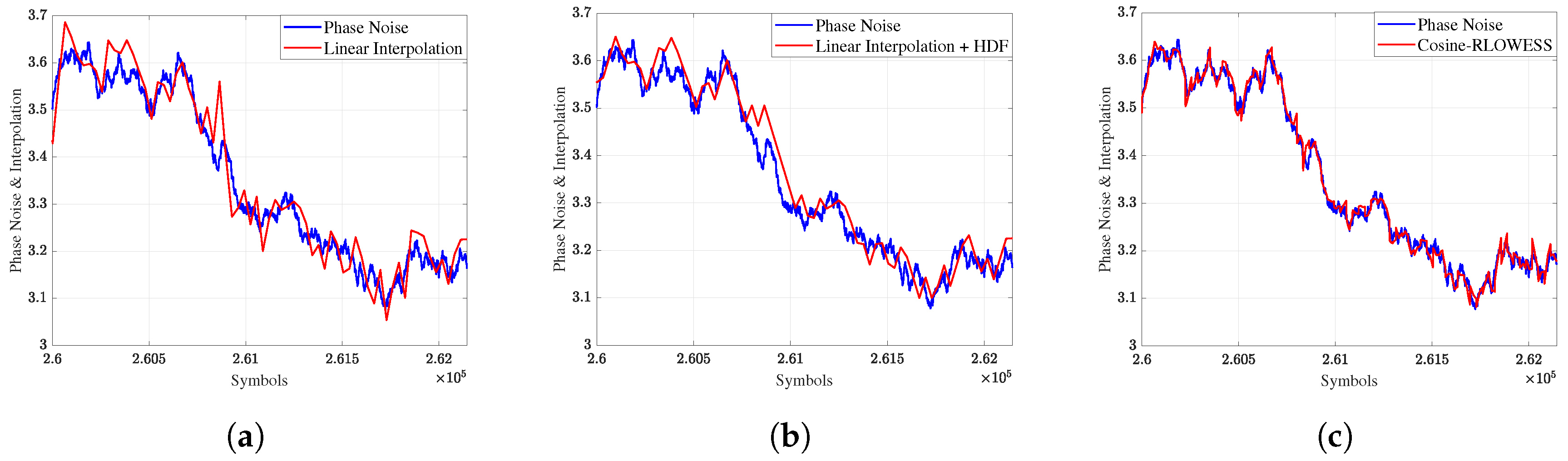
In Figure 6, we present the phase tracking analysis. This figure highlights the effectiveness of the hard-decision filter, as depicted in Figure 6b, in reducing peak values during the tracking process. Compared to the results produced by the pure linear interpolator in Figure 6a, the application of this hard-decision filter significantly attenuates the peaks. However, the tracking is not entirely smooth. In contrast, the results obtained using the robust interpolator, shown in Figure 6c, show much smoother phase tracking. This comparison clearly demonstrates the superiority of the RLOWESS method over other interpolation techniques for phase tracking.

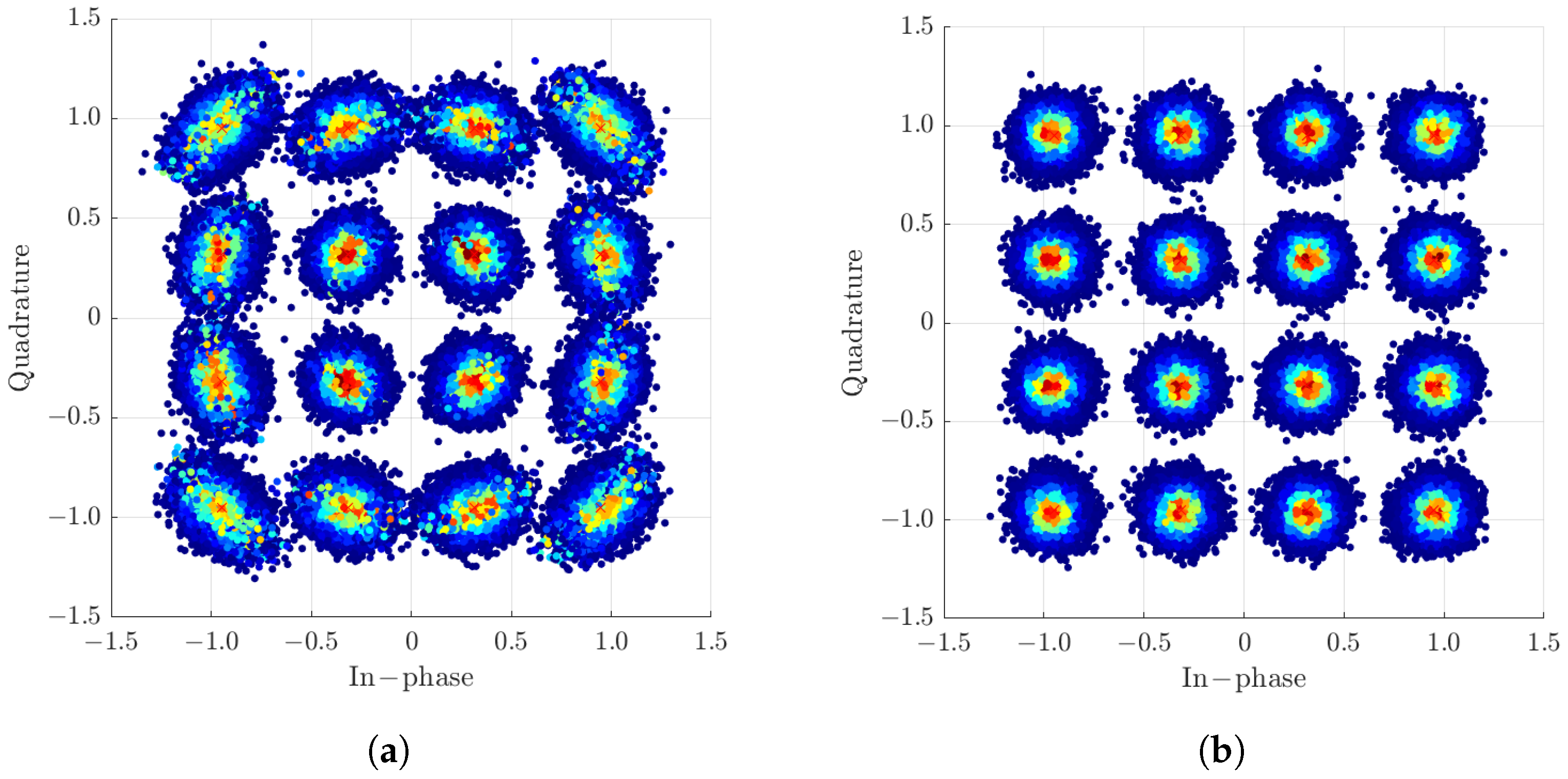
In Figure 7, the results of the 16QAM constellation after phase recovery are illustrated, comparing two interpolation methods. Figure 7, on the left, shows the constellation after phase recovery using the linear method combined with a hard-decision filter. In particular, the symbols at the outer edges of the constellation exhibit significant elongation, indicating distortion in the recovered symbols. In contrast, Figure 7, on the right, presents the scenario in which pilot symbols have been removed and carrier recovery has been performed using a cosine filter in conjunction with the robust locally weighted smoothing interpolation method (Cosine-RLOWESS). Here, the external symbols appear in a Gaussian format, demonstrating that smoother phase recovery is crucial for effective carrier phase recovery. This improvement will have a significant impact on the subsequent analysis of the bit error rate.

A key conclusion from the constellation analysis is that the hard-decision filter-based interpolator exhibits a notable disadvantage: it causes elongation in the outer symbols. However, this limitation can be alleviated by using probabilistic shaping techniques. These techniques reduce the probability of symbols occupying these outer regions, while leveraging the simplicity and efficiency of linear interpolation.

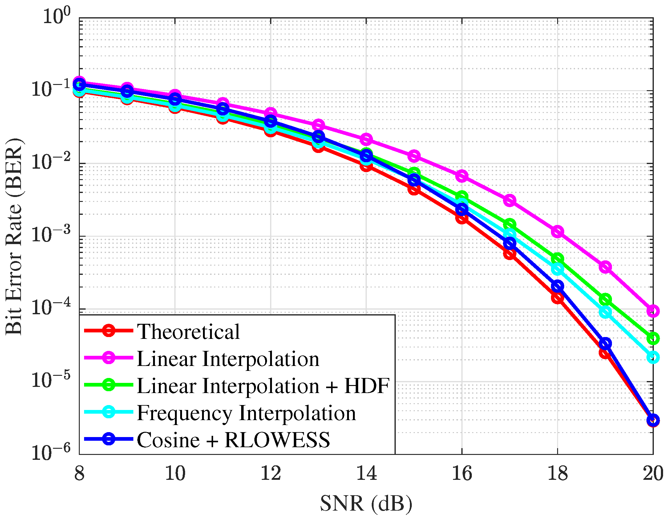
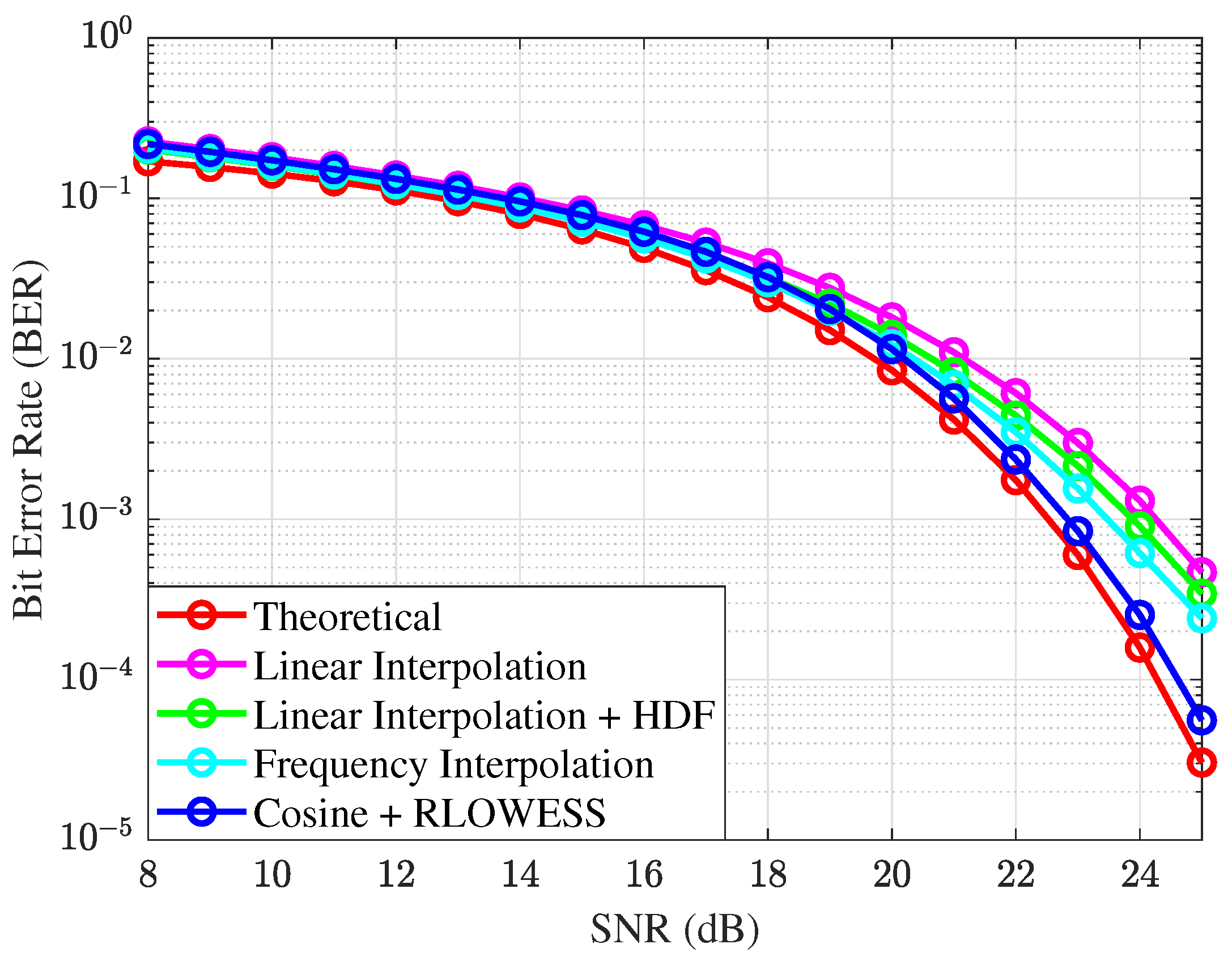
In the BER vs. SNR analysis, shown in Figure 8, we evaluate the performance of various CPR algorithms with interpolation for 16QAM modulation. The system operates with a linewidth of $\Delta \nu =100\times 2\mathrm{kHz}$ and a symbol rate of 50 Gbaud. Among the algorithms considered, the linear interpolator exhibits the weakest performance but serves as a valuable reference for benchmarking system improvements. The theoretical curve represents the performance of BER in the presence of pure ASE noise, modeling the bit error rate (BER) for M-QAM modulation in an AWGN channel when phase noise is absent.

Notably, the incorporation of a hard-decision filter enhances the linear interpolator’s performance, particularly at SNR values below 13 dB, demonstrating the utility of straightforward implementations. However, as the SNR increases, the effectiveness of the hard-decision filter diminishes. This reduction in performance is likely due to the filter’s reliance on fixed thresholds, which are sensitive to variations in power levels, affecting noise power estimation and outlier detection. Consequently, these power fluctuations lead to variability in the BER.

To address these issues and improve the reliability of the system, we transitioned from a hard-decision approach to a more sophisticated filtering technique. A cosine filter was selected because of its proven effectiveness in achieving smoother interpolation. The combination of a cosine filter and robust locally weighted regression yields consistently impressive results across the entire SNR spectrum, demonstrating excellent stability. The efficiency of this algorithm is further enhanced by its burst analysis approach, which utilizes pilot symbols and eliminates the need for complete signal analysis to achieve effective tracking. In particular, a BER of ${10}^{-3}$ is achievable at approximately 17 dB SNR, as shown by the blue line in Figure 8, which is remarkably close to the theoretical value. This result is based on the analysis of a signal containing $2^{18}$ symbols.

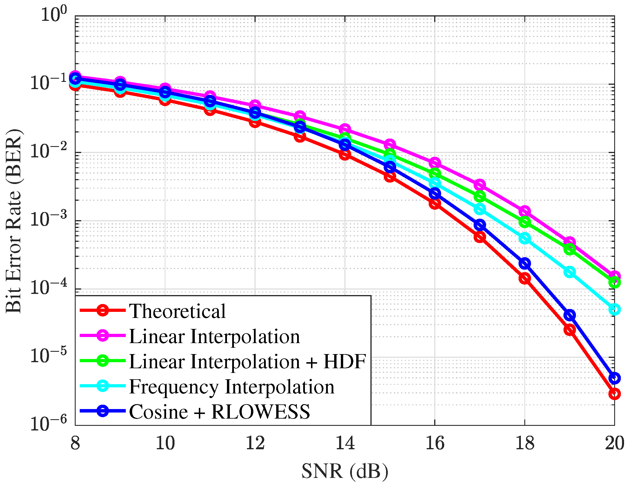
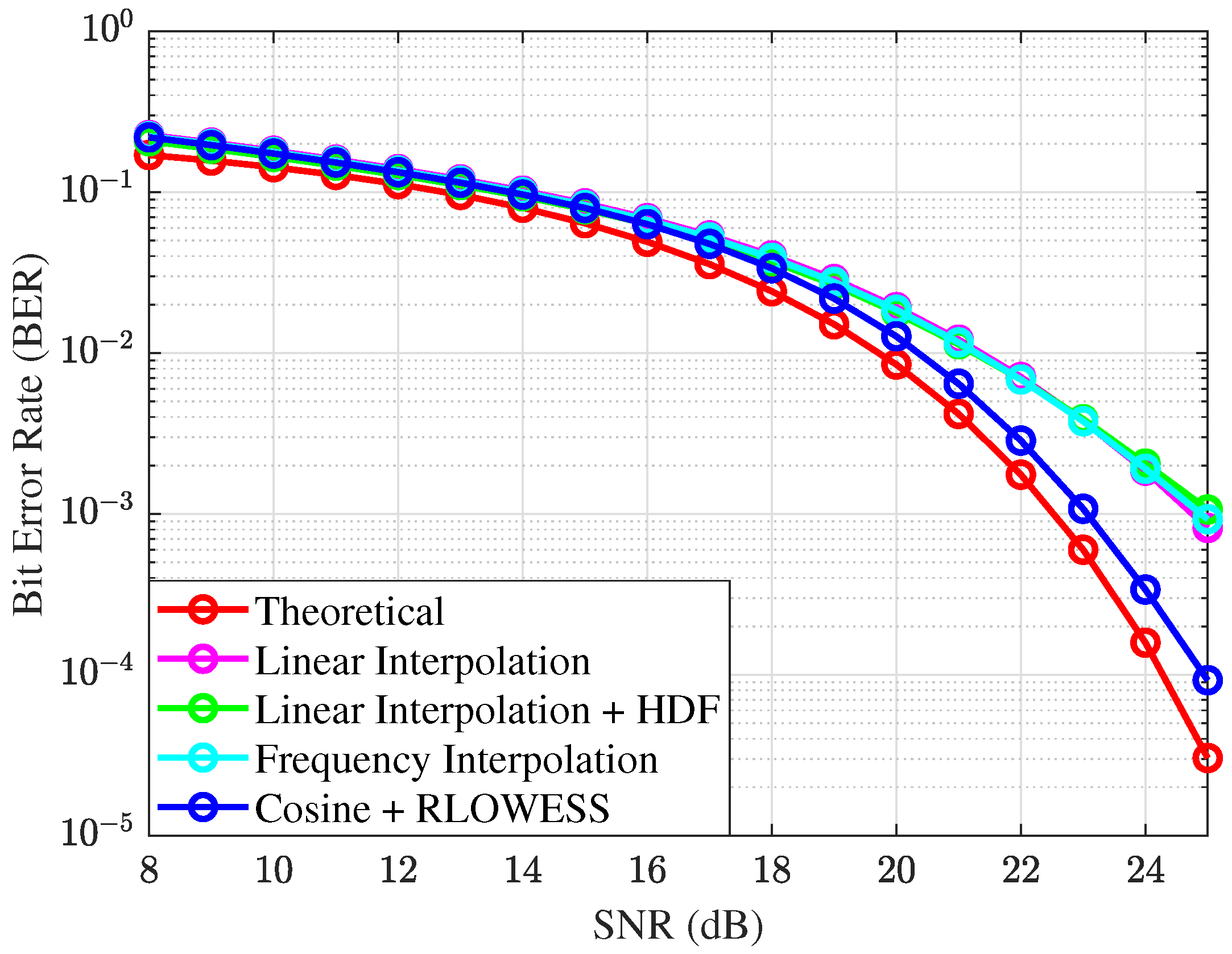
In Figure 9, the phase noise increases to $\Delta \nu =400\times 2\mathrm{kHz}$ with a symbol rate of $50\mathrm{Gbaud}$. To prevent frequency filter interpolation from experiencing losses, as observed in Figure 9 as an increase in signal-to-noise ratio (SNR), which may indicate a stability issue, the passband width is expanded to $150\mathrm{MHz}$. As a result, the filter continues to perform effectively within the defined linewidth of $\Delta \nu =400\times 2\mathrm{kHz}$.

Among the algorithms evaluated, the combination of the cosine filter and RLOWESS (Cosine-RLOWESS) consistently delivers the best performance across the entire range of SNR values. Although an increase in phase noise leads to greater losses, these losses are effectively mitigated by the advanced processing capabilities of the Cosine-RLOWESS algorithm.

The results for $\Delta \nu =100\times 2\mathrm{kHz}$, a symbol rate of $50\mathrm{Gbaud}$, and a modulation order of $64\mathrm{QAM}$ are illustrated in Figure 10. The analysis shows that the linear interpolation algorithm, when combined with a hard-decision filter, performs acceptably at lower SNR values. However, as the SNR increases, certain limitations of both hard-decision filters and frequency interpolators become apparent. In contrast, the system that demonstrates stability across a wide range of SNR values is the linear interpolator combined with the cosine and RLOWESS techniques.

The behavior of the interpolators remains consistent when the linewidth is increased to $\Delta \nu =400\times 2\mathrm{kHz}$ at the given symbol rate, as illustrated in Figure 11. A significant modification to the frequency interpolator was made by expanding its bandwidth to $450\mathrm{MHz}$, resulting in better performance. However, issues previously observed at the bandwidth edges reappeared despite this adjustment. Therefore, it can be concluded that the interpolator that combines the cosine and RLOWESS filters consistently outperforms the others.

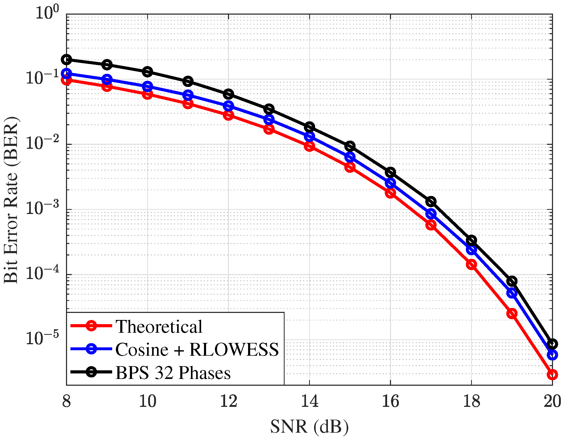
In Figure 12, the parameters are set as follows: $\Delta \nu =800\times 2\mathrm{kHz}$, a symbol rate of $50\mathrm{Gbaud}$, and a modulation order of $16\mathrm{QAM}$. On the basis of previous results, the Cosine-RLOWESS technique has been established as the reference interpolator. Here, its performance is compared to a blind phase search (BPS) algorithm using 32 phases, which is suitable for improved performance with 16QAM. The Cosine-RLOWESS interpolator demonstrates stable performance across the entire SNR range, consistently outperforming the BPS algorithm.

At approximately $16\mathrm{dB}$ SNR, the Cosine-RLOWESS interpolator shows a gain of $0.5\mathrm{dB}$ over the BPS algorithm. A key advantage of the Cosine-RLOWESS method is its ease of reconfiguration. In contrast, as will be discussed later, changing the modulation scheme with the BPS algorithm requires reconfiguring its differential encoding.

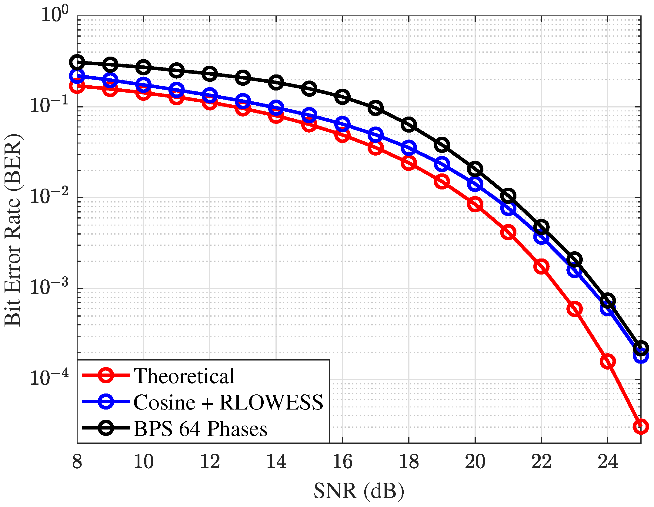
In Figure 13, the modulation order is increased to 64QAM, and the phase search is expanded to 64 phases, meeting the minimum requirements for this modulation type, which typically requires at least 32 phases [1]. These results align with previous observations for the 16QAM constellation. At an SNR of $23\mathrm{dB}$, the Cosine-RLOWESS interpolator achieves a gain of $0.2\mathrm{dB}$ over the BPS algorithm at a BER of $1\times {10}^{-3}$. However, as the SNR increases and $\Delta \nu T_s$ grows, the performance gap between algorithms diminishes. However, the Cosine-RLOWESS method continues to demonstrate stability across the entire SNR range, underscoring its robustness.

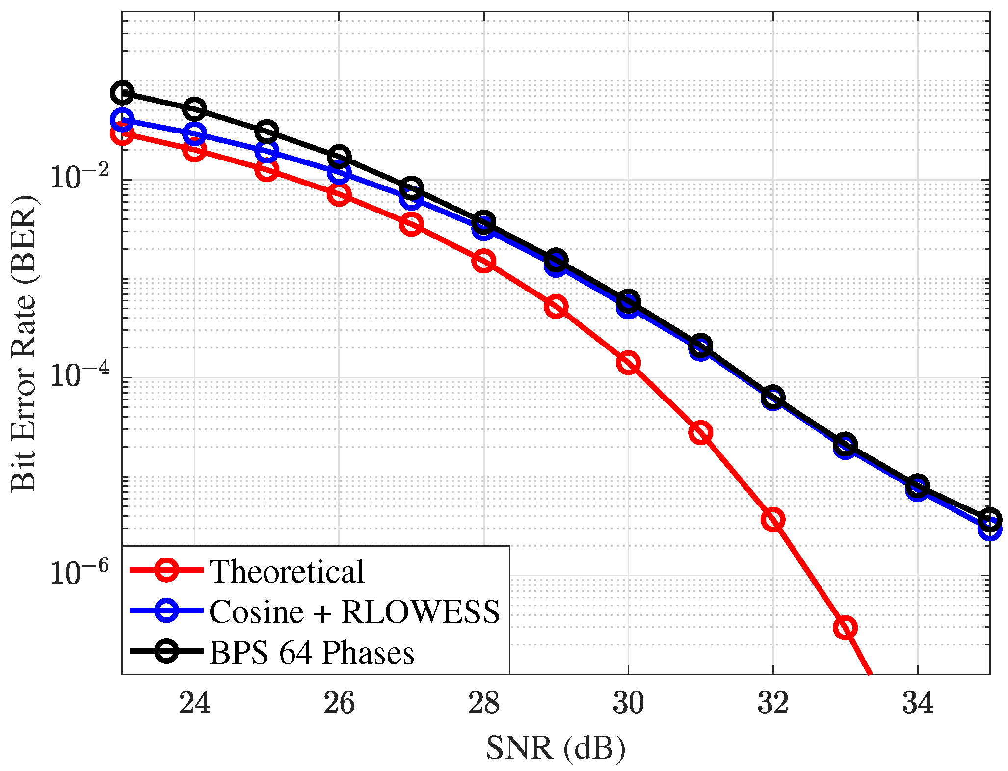
In Figure 14, the parameters are set as follows: $\Delta \nu =200\mathrm{kHz}\times 2$, a symbol rate of $50\mathrm{Gbaud}$, and a modulation order of 256QAM. These values are consistent with the requirements of the modulation format. Although there are visible differences compared to the theoretical curve, the Cosine-RLOWESS interpolator achieves results comparable to those of the BPS algorithm. These findings suggest that the Cosine-RLOWESS interpolator performs optimally with lower modulation orders and smaller linewidths. However, with higher modulation orders such as 256QAM and significant linewidth effects, its performance converges with that of the BPS algorithm.

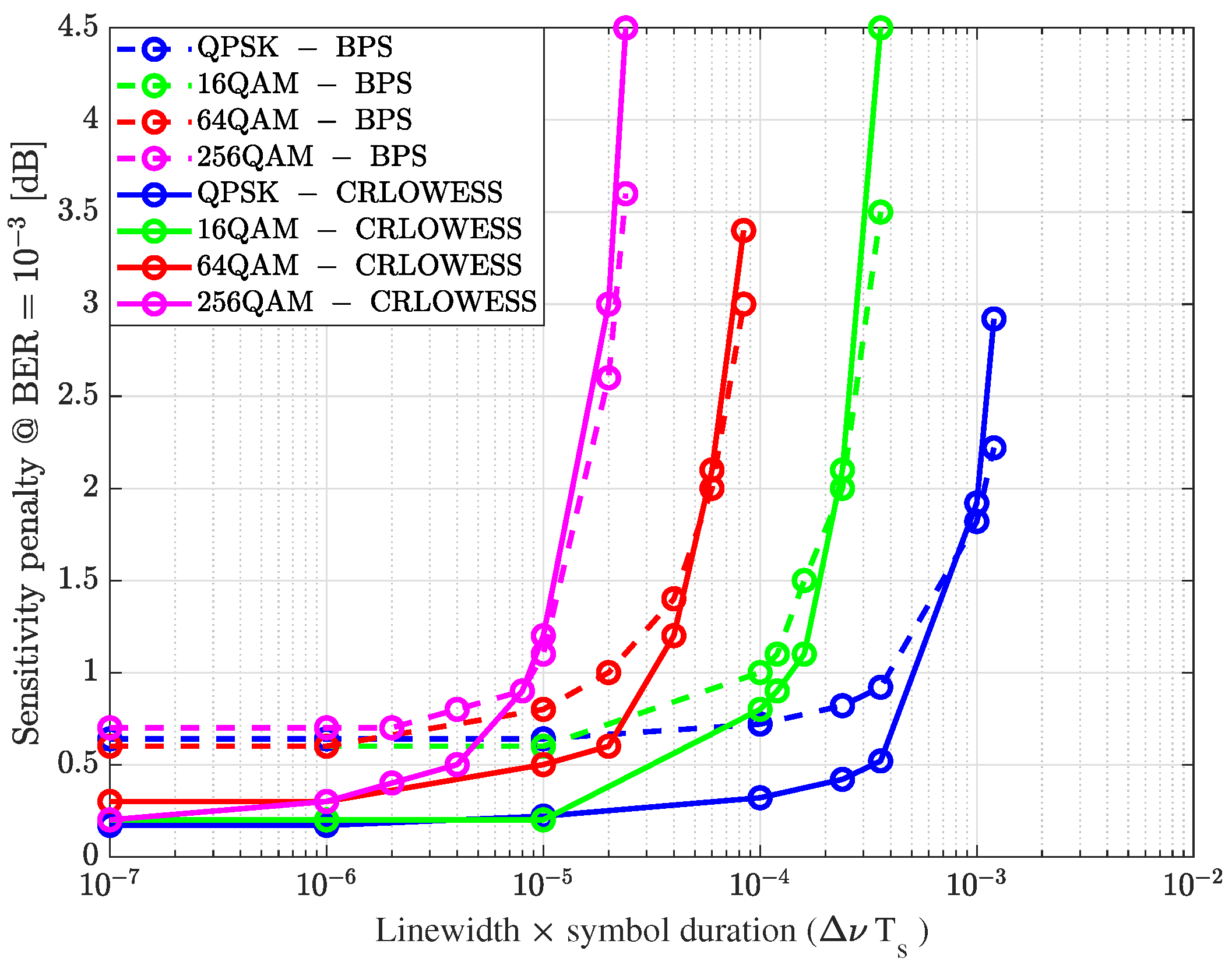
Figure 15 illustrates the sensitivity penalty at a BER of ${10}^{-3}$ for different modulation formats when compensating for phase noise using the BPS and Cosine-RLOWESS algorithms. The Cosine-RLOWESS algorithm demonstrates strong robustness against low values of $\Delta \nu T_s$. Specifically, for the QPSK, 16QAM, and 64QAM modulation formats, the sensitivity penalty in dB is consistently lower compared to BPS [1,32,39], particularly when $\Delta \nu T_s$ is below ${10}^{-5}$. This indicates that employing advanced laser oscillators with finely tuned linewidths could offer significant advantages [38]. Furthermore, in the design of low-margin optical networks, adjusting the data rate according to demand can help to maintain $\Delta \nu T_s$ within an optimal range.

As the modulation order and linewidth increase, the performance of Cosine-RLOWESS converges with that of BPS. For higher values of $\Delta \nu T_s$—such as when the symbol period decreases or the laser linewidth increases to several megahertz—BPS demonstrates better tolerance. However, the Cosine-RLOWESS algorithm offers the advantage of a lower complexity compared to BPS, as reflected in the reduced processing time discussed in Section 4.

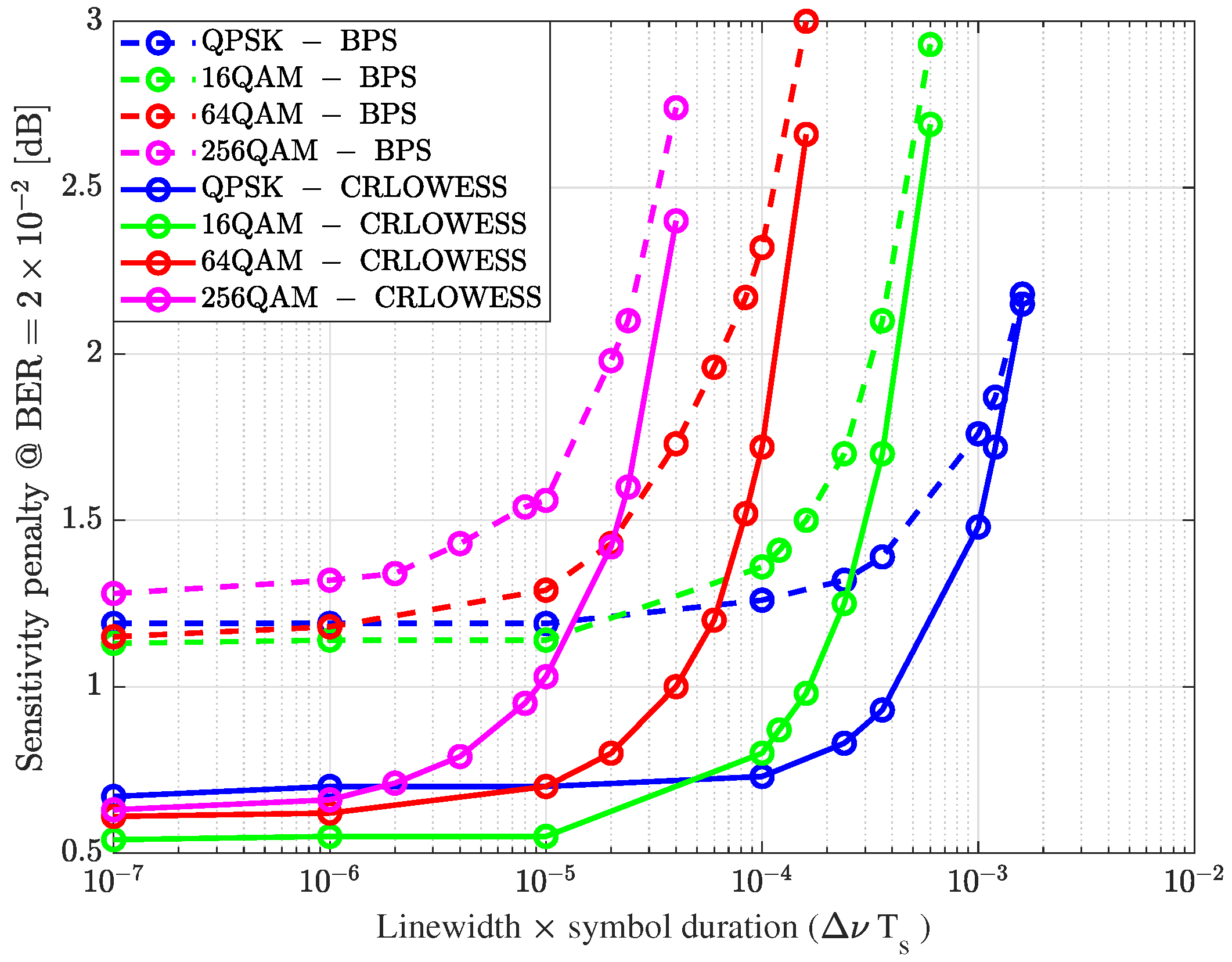
Advances in forward error correction (FEC) algorithms allow for more flexible bit error rate (BER) thresholds, particularly when FEC is not employed. Specifically, new approaches are shifting from traditional hard-decision methods to soft-decision methods, or a combination of both, to improve overall system performance. As noted in [40], setting a fixed BER threshold should be avoided, especially when using soft-decision decoding. Instead of relying on the BER threshold, it is recommended to use generalized mutual information (GMI) as a more accurate reference metric.

However, when hard-decision decoding is used, setting a BER threshold remains a valid approach. Traditionally, this threshold has been set to $3.8\times {10}^{-3}$. According to [41], the hard-decision FEC thresholds can reach $2.24\times {10}^{-2}$, but achieving a post-FEC BER of ${10}^{-15}$ requires an overhead of 33.33%. Based on these findings, we set the sensitivity to a minimum BER of $2\times {10}^{-2}$. Figure 16 presents the sensitivity results for the blind phase search algorithm (BPS) and the Cosine-RLOWESS method.

The Cosine-RLOWESS consistently outperforms the BPS algorithm, even at a sensitivity level corresponding to a BER of $1\times {10}^{-3}$. Specifically, across all constellations compared, the Cosine-RLOWESS algorithm exhibits superior performance when the product $\Delta \nu T_s$ is very low or extremely high. This advantage enables the system to support higher laser linewidth values more effectively.

As mentioned above, using these hard-decision decoding values requires an increase in overhead. Therefore, it is important to consider the trade-off between the minimum required BER and the maximum allowable overhead in practical scenarios. In Figure 16, with a BER of $2\times {10}^{-2}$, the Cosine-RLOWESS algorithm consistently outperforms the BPS algorithm. For example, with a linewidth of $\Delta \nu =2500\mathrm{kHz}$ and a symbol rate of $R_S=50\mathrm{Gbaud}$, corresponding to $\Delta \nu T_s=1\times {10}^{-4}$, the performance difference is 0.56 dB for 16QAM and increases to 0.6 dB for 64QAM. As the sensitivity curves indicate, this performance gap becomes more pronounced as the laser linewidth narrows.

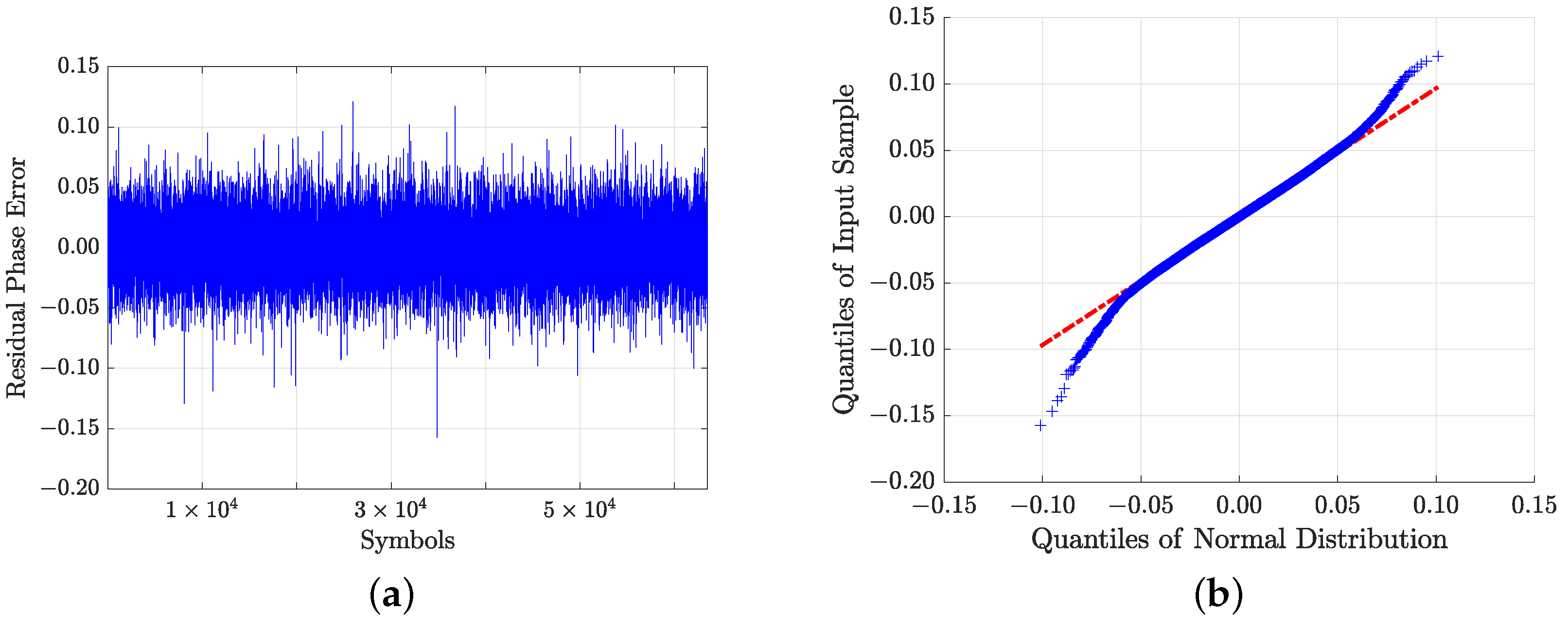
Figure 17a analyzes the residual phase noise, which is calculated as the difference between the phase noise and the output of a tracking algorithm using the Cosine-RLOWESS method. The residual noise is influenced primarily by two factors: the variance of the phase noise and the signal-to-noise ratio (SNR). Occasionally, spurious values appear that are not directly caused by phase noise errors but resemble Gaussian channel noise, particularly near the quadrant boundaries in the constellation diagram. To mitigate this, an algorithm is implemented to detect and correct phase jumps by referencing the previous symbol, resulting in a more realistic representation of the residual phase noise.

Figure 17b shows the quantile–quantile plot that compares residual noise quantiles against the theoretical quantiles of a normal distribution, using the Cosine-RLOWESS interpolator. A linear pattern in this plot suggests that the residual noise follows a normal distribution. However, at higher noise variance, observable at an SNR of $25\mathrm{dB}$, with a linewidth of $\Delta \nu =800\mathrm{kHz}$, a symbol rate of $R_s=50\mathrm{Gbaud}$, and a modulation order of 64QAM, the plot’s extremities begin to diverge. This divergence indicates variability in phase noise differences near the boundaries, particularly around a value of $\pm 0.15$. This value can fluctuate on the basis of the overall phase noise variance, and in more degraded environments the quantiles may exhibit extreme peaks at the edges.

4. Computational Complexities

The use of pilot symbols in coherent optical communication systems has been investigated for cycle slip analysis [42,43], as a way to avoid differential coding. Cycle slips are particularly common in long-range communication systems. As discussed in the Introduction, the overhead for pilot symbols is set at 3% of the total transmitted symbols, resulting in an SNR penalty of $0.13\mathrm{dB}$. This penalty is calculated using the formula ${\displaystyle \frac{P}{P+D}}$, where P represents the length of the pilot sequence and D represents the length of the transmitted data. These studies highlight that the main drawback of using pilot symbols is the reduction in spectral efficiency, which is why an overhead of up to 5% is recommended.

The BPS algorithm is widely recognized as a benchmark for carrier recovery processing. However, its computational complexity is significantly affected by the relationship between the number of test phases and the modulation order. Specifically, the number of test phases scales as $2^4$, $2^5$, and $2^6$ for 16QAM, 64QAM, and 256QAM, respectively, leading to high computational demands. Various studies have focused on improving the efficiency of BPS implementation, often combining techniques in two stages, as demonstrated in [44]. Furthermore, the use of differential coding in BPS presents additional challenges, which has led recent research to explore alternative approaches. One promising solution is the use of recursive probability weighting based on phase variance levels, which can reduce the number of test phases required [45].

The BPS algorithm works by testing a set of discrete phase values across the received signal block and selecting the phase that minimizes a cost function, typically related to the magnitude of the error vector. The computational complexity of BPS is driven primarily by the phase testing stage, resulting in a complexity of $\mathcal{O}\left(NB\right)$. This means that complexity scales linearly with the number of test phases, B, and the size of the processed symbols, N, which makes BPS computationally expensive compared to other phase estimation methods, where the selection of N and B can significantly influence both the performance of the algorithm and its computational burden.

For the Cosine-RLOWESS interpolation method, the first step involves extracting the pilot symbols and phase information from the input signal. This process results in a computational complexity of $\mathcal{O}\left(N\right)$, where N represents the total number of symbols, indicating that the algorithm has a linear computational complexity.

The LOWESS method involves locally weighted regression over a sliding window that moves across the data points. The computational complexity of this method depends on the number of operations performed for each data point within its local window. Generally, the complexity is $\mathcal{O}\left(nm\right)$, where n represents the number of points to smooth and m denotes the span or window size, which corresponds to the number of points used in each local regression. Typically, m is much smaller than n, and its effect is most significant when it constitutes a substantial fraction of n.

In this context, n refers to the pilot spacing and m is set to 5% of that length. If m is considered constant for practical purposes or is restricted to a small fraction of n, the complexity can be approximated as $\mathcal{O}\left(n\right)$.

Since the LOWESS method is applied to the entire set of N symbols, the overall computational complexity of the algorithm becomes $\mathcal{O}\left(N\right)\times \mathcal{O}\left(mn\right)=\mathcal{O}\left(Nmn\right)$. Assuming that m and n are independent of N and each other, and since m is small and can be treated as a constant, the complexity depends primarily on how n scales with respect to N. Consequently, the overall complexity can still be simplified to $\mathcal{O}\left(N\right)$ when considering practical scenarios.

$$\mathcal{O}\left(Nn\right).$$

(22)

Therefore, the overall computational complexity for running both processes one after the other is as follows:

$$\mathcal{O}\left(N\right)+\mathcal{O}\left(Nn\right)=\mathcal{O}\left(Nn\right).$$

(23)

This means that, for large values of N, the term $\left(Nn\right)$ dominates, and thus represents the overall growth rate of the computational workload.

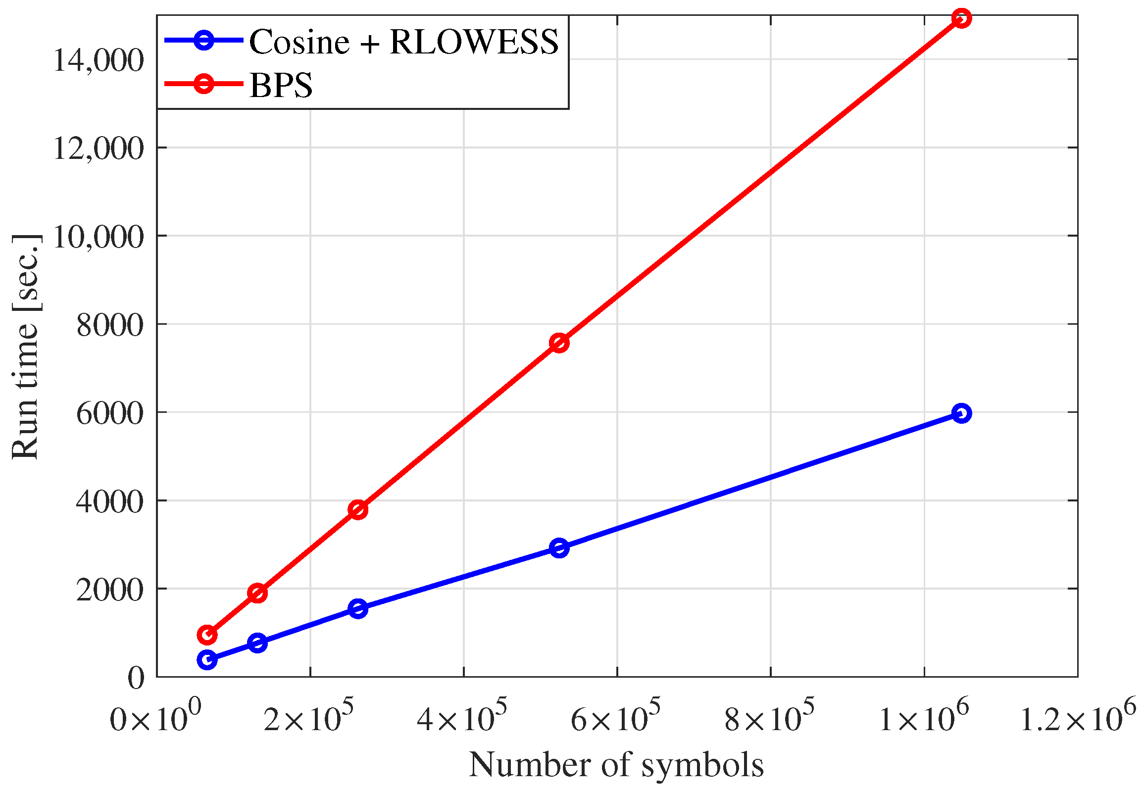
Figure 18 compares the run times of the Cosine-RLOWESS and BPS algorithms, providing information on their relative performance under identical conditions. Although run times are influenced by factors such as processor speed and memory, this analysis ensures a fair assessment by standardizing parameters. The evaluation focuses on the impact of varying the number of input symbols while maintaining consistent phase noise and modulation settings. Specifically, 64QAM modulation is used with a linewidth of $\Delta \nu =800\mathrm{kHz}\times 2$ and a symbol rate of $R_s=50\mathrm{Gbaud}$. The input symbol count ranges from $2^{16}$ to $2^{20}$, with the number of test phases for the BPS algorithm set to 64 and the filter length set to 12.

The results indicate that the Cosine-RLOWESS algorithm consistently achieves shorter run times across all input sizes compared to the BPS algorithm. Moreover, the Cosine-RLOWESS algorithm demonstrates a computational complexity increase that is approximately $50\%$ lower than that of the BPS algorithm, making it a more efficient choice for managing phase noise as computational demands grow.

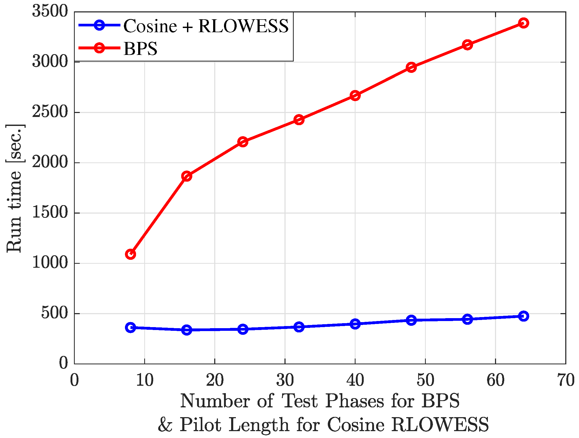
Figure 19 presents a comparative analysis of the run times of the BPS and Cosine-RLOWESS algorithms under varying conditions. For the BPS algorithm, the filter length is fixed at 12, while the number of test phases is varied. As anticipated, increasing the number of test phases improves the precision of the results but also leads to a corresponding increase in run time, as shown in the figure.

For the Cosine-RLOWESS algorithm, we evaluated the impact of varying pilot symbol lengths, ranging from short lengths (8 symbols) to longer lengths (64 symbols). Unlike the BPS algorithm, reducing the pilot length increases precision, but at the cost of spectral efficiency. A pilot length of 32 symbols strikes a favorable balance, delivering satisfactory precision with only a minimal increase in run-time, thus having a negligible impact on the algorithm’s overall efficiency. Although a pilot length of 16 symbols improves performance, it results in a 6.6% loss in spectral efficiency, which is prohibitive. Therefore, we conclude that the Cosine-RLOWESS algorithm offers significant advantages in computational efficiency and run time, making a pilot length of 32 symbols an optimal choice.

The run-time analysis indicates that integrating the BPS algorithm with pilot burst mode transmission in optical communications is not only feasible but also shows considerable potential to improve performance in specific scenarios.

5. Discussion

In this section, we analyze the results of our study and compare them with related work in the field. Most existing carrier phase estimation (CPE) algorithms rely on pilot symbols for assistance, which can slightly increase system complexity and, for most practical applications, only slightly reduce the overall information rate [27]. In contrast, blind phase estimation methods, such as the blind phase search (BPS) algorithm [1] and the Viterbi–Viterbi phase estimator (VV-PE) [22], eliminate the need for pilot symbols. However, VV-PE requires adaptation for higher-order modulation formats, while BPS, despite being modulation-format-independent, suffers from high computational complexity. Moreover, both methods are vulnerable to severe burst errors caused by cycle slips, which can significantly degrade the system performance [25].

In our research, we analyze the advantages of eliminating outliers in phase tracking, as their presence degrades the accuracy of the interpolator, thereby affecting phase recovery. This effect is evident in Figure 6. Among the interpolation methods considered, RLOESS and RLOWESS provide the best fit, the latter being selected because of its ability to introduce greater flexibility in modifying the weights. This flexibility offers more control over the smoothing process, allowing for the fine-tuning of phase correction, which is particularly beneficial in more challenging scenarios.

Figure 6 illustrates the benefits of incorporating a filter into the interpolator. The process begins with the hard-decision filter, shown in Figure 6b, and culminates in a smooth interpolation achieved through the combination of the cosine function and the RLOWESS interpolator, as depicted in Figure 6c.

Furthermore, Figure 8 presents a comparison of different interpolators with the theoretical curve, which represents the performance of a communication system without phase noise disturbances. In this scenario, the only impairment is amplified spontaneous emission (ASE) noise, modeled as additive white Gaussian noise (AWGN) in the channel.

Although the frequency domain interpolator shows good performance, as discussed in [25], its implementation complexity is significantly high. Computing the FFT requires a substantial portion of the signal, making this approach less practical for real-time applications.

For instance, when the modulation order increases or when phase noise is exacerbated by an increase in the laser linewidth to $\Delta \nu =2\times 400$ kHz, an adjustment in the bandwidth of the frequency filter becomes necessary to maintain acceptable performance. Specifically, the filter bandwidth must be increased from 150 MHz to 450 MHz to compensate for the increased phase noise. The impact of this adjustment on system performance is illustrated in Figure 11.

In contrast, the Cosine-RLOWESS method provides a more efficient solution for phase noise tracking while maintaining lower computational complexity, making it suitable for real-time implementations. In this approach, the tracking is performed based only on a slot portion of the signal, unlike the frequency-filter approach.

In our system, the spacing of the pilot symbols was set to a ratio of 1:32, corresponding to $3\%$ of the transmitted symbols. It is interesting to compare this pilot symbol configuration with related studies, such as Cao et al. [46], which uses the aiding Kalman filter (AKF) as the carrier phase estimation (CPE) algorithm. The ratios of pilot symbols used in their study are relatively very high (1:1, 1:3, and 1:7), thus limiting the power and spectral efficiencies, while the Cosine-RLOWESS method maintains acceptable power and spectral efficiencies for pilot-based systems, within the recommended maximum overhead of up to $5\%$ [42,43,47].

In general, studies that use pilot symbols exhibit significantly lower computational complexity, as reported in [9,27,46]. Another key advantage is the ability to mitigate cycle slips without requiring differential coding. For example, in [9], the authors propose an improved carrier phase estimation (CPE) method that employs dual pilot tones to suppress equalization-enhanced phase noise (EEPN) while mitigating cycle slips. Compared to the BPS algorithm, this approach introduces additional filtering and pilot tone processing, but eliminates the need for complex phase correction. Similarly, Cosine-RLOWESS inherently resists cycle slips, as discussed in the introduction of Section 4.

In Section 4, we compared the computational complexity of the Cosine-RLOWESS and BPS algorithms.

The blind phase search (BPS) algorithm employs a brute-force phase estimation approach, where multiple test phase angles are applied to the received symbols, and the optimal phase is selected. The primary computational components of BPS are as follows [1,32]:

• Multiplications: Each test phase requires a phase rotation (complex multiplication), leading to a complexity of $\mathcal{O}\left(NB\right)$.
• Additions: Computing the phase error metric in all test phases scales as $\mathcal{O}\left(NB\right)$.
• Comparisons: Selecting the best phase requires additional comparisons, adding a complexity of $\mathcal{O}\left(B\right)$.

Thus, the total computational complexity of BPS is given by $\mathcal{O}\left(NB\right)$. In contrast, the Cosine-RLOWESS method reduces the computational complexity to $\mathcal{O}\left(Nn\right)$, where n represents the pilot spacing.

Overall, the proposed algorithm is computationally more efficient than BPS, particularly for high-order modulation formats, where BPS requires a large B, making it computationally expensive.

A comparison of Cosine-RLOWESS with other pilot-based algorithms is summarized in

Table 1. Computational complexity comparison of CPE algorithms based on pilot symbols.

Algorithm	Multiplications (MULT)	Additions (ADD)
CMA+BPS [46]	$16M+16+6NB+4N$	$16M+4+6NB-B+2N+2$
AKF [46]	585	459
2-Stage BPS [27]	$6NBT+4N$	$5NBT+2N+3$
PCPE [27]	$10N+8$	$6N+3$
MPD-BPS [27]	$12NBT$	$21N$
UKF [27]	$56N$	$264N$
EKF-PC [27]	$56N$	$88N$
Cosine-RLOWESS	$\mathcal{O}(Nlogn)$	$\mathcal{O}\left(N\right)$

.

Table 1 compares the computational complexity of various carrier phase estimation (CPE) algorithms, including methods based on Cosine-RLOWESS, BPS, and Kalman.

Compared to extended Kalman filtering (EKF-PC) and unscented Kalman filtering (UKF), Cosine-RLOWESS has a lower computational burden, particularly in high-order modulation formats, where Kalman-based methods require matrix operations. However, potential performance trade-offs should be considered, as Kalman filtering techniques may offer superior phase noise tracking under highly dynamic conditions.

The AKF algorithm maintains a fixed complexity of $\mathcal{O}\left(N\right)$, as stated in Table 1, since it processes symbols sequentially with a constant computational cost. In contrast, the general Cosine-RLOWESS has a complexity of $\mathcal{O}\left(Nn\right)$, where n denotes the pilot spacing.

Since n is typically a slot of N, the computational cost of Cosine-RLOWESS is slightly higher than that of AKF, especially as the number of pilot symbols increases. However, for small values of n, its complexity remains close to $\mathcal{O}\left(N\right)$, making Cosine-RLOWESS a computationally viable alternative.

Overall, while AKF is more efficient in terms of computational complexity, Cosine-RLOWESS may offer advantages in phase noise robustness, depending on the pilot symbol density and modulation order. Moreover, it achieves a superior spectral and power efficiencies compared to AKF approaches.

Furthermore, Cosine-RLOWESS provides a computationally efficient alternative to BPS for phase estimation, particularly in high-order modulation formats, while maintaining a lower complexity compared to Kalman-based approaches.

6. Conclusions

An efficient, low-complexity, pilot-assisted phase estimation technique has been presented for coherent optical receivers. This method is based on a robust interpolation technique designed for quasioptimal operation, offering improved phase estimation accuracy. It effectively addresses the unique challenges posed by new scenarios in optical communication systems. We conducted comprehensive simulations to demonstrate the performance of the method compared to conventional techniques, highlighting the improvements in the curves of BER as a function of SNR and in the penalties in SNR at the pre-FEC BER thresholds of 1.0 × 10⁻³ and 2.0 × 10⁻².

The proposed Cosine-RLOWESS interpolation outperforms all other pilot-assisted interpolation techniques studied across entire ranges of SNRs. In fact, the BERxSNR curves for the Cosine-RLOWESS method are very close to the optimal AWGN channel curves. The Cosine-RLOWESS method surpasses BPS in all cases throughout the SNR range, except in the higher range of SNR > 28 dB for 256QAM, where both algorithms performed equally well. We show the sensibility penalties incurred by the BPS and Cosine-RLOWESS methods at a pre-FEC BER of 1.0 × 10⁻³, respectively. First, we observe that the breakdown thresholds for $\Delta \nu T_s$, above which there is an exponential increase in the sensitivity penalties, are approximately the same for all the respective modulation formats (QPSK, 16QAM, 64QAM, and 256QAM) for both the BPS and Cosine-RLowess methods. However, in the flat working region for $\Delta \nu T_s$ below the breakdown thresholds for the four modulation formats, the Cosine-RLOWESS sensibility penalties are approximately 0.42 dB (QPSK), 0.4 dB (16QAM), 0.3 dB (64QAM), and 0.3 dB (256QAM) lower than the corresponding penalties for the BPS algorithm. For a pre-FEC BER of 2.0 × 10⁻², there is an even greater improvement in the Cosine-RLOWESS sensibility penalties.

In summary, the simulation results show a significant performance improvement of the Cosine-RLOWESS method compared to other linear interpolation methods and the BPS algorithm. Moreover, the proposed pilot-assisted method avoids cycle slips, presents low computational complexity, and can be applied to probabilistic shaping modulation, where the BPS fails at optimal operational distributions.