Dynamic Indoor Visible Light Positioning and Orientation Estimation Based on Spatiotemporal Feature Information Network

Abstract

Visible Light Positioning (VLP) has emerged as a pivotal technology for industrial Internet of Things (IoT) and smart logistics, offering high accuracy, immunity to electromagnetic interference, and cost-effectiveness. However, fluctuations in signal gain caused by target motion significantly degrade the positioning accuracy of current VLP systems. Conventional approaches face intrinsic limitations: propagation-model-based techniques rely on static assumptions, fingerprint-based approaches are highly sensitive to dynamic parameter variations, and although CNN/LSTM-based models achieve high accuracy under static conditions, their inability to capture long-term temporal dependencies leads to unstable performance in dynamic scenarios. To overcome these challenges, we propose a novel dynamic VLP algorithm that incorporates a Spatio-Temporal Feature Information Network (STFI-Net) for joint localization and orientation estimation of moving targets. The proposed method integrates a two-layer convolutional block for spatial feature extraction and employs modern Temporal Convolutional Networks (TCNs) with dilated convolutions to capture multi-scale temporal dependencies in dynamic environments. Experimental results demonstrate that the STFI-Net-based system enhances positioning accuracy by over 26% compared to state-of-the-art methods while maintaining robustness in the face of complex motion patterns and environmental variations. This work introduces a novel framework for deep learning-enabled dynamic VLP systems, providing more efficient, accurate, and scalable solutions for indoor positioning.

1. Introduction

The rapid development of technologies such as industrial Internet of Things (IoT), intelligent robotics, and Automated Guided Vehicles (AGVs) has created an urgent demand for high-precision indoor positioning systems, which have become core demands for intelligent manufacturing, smart warehousing, and logistics scheduling [1,2,3,4]. Visible Light Positioning (VLP), as an emerging solution, utilizes LED signals for target positioning and orientation tracking, offering high stability, low carbon emissions, and wide coverage. These advantages provide superior accuracy and spatial resolution compared to traditional positioning technologies such as Wi-Fi, Bluetooth, and infrared.

VLP systems can be classified into two main categories based on the receiver type: photodiode (PD)-based and CMOS image sensor-based configurations. PD-based VLP (PD-VLP) is particularly well-suited for large-scale IoT deployments due to its low cost, energy efficiency, and privacy protection. In contrast, CMOS-based solutions face limitations in position sensitivity, high computational demands, and privacy concerns, despite offering potential precision benefits. By exploiting simplified light-intensity-to-position models and leveraging the inherent angular sensitivity of PDs, PD-VLP enables joint 6-DoF (Degrees of Freedom) estimation of both position and orientation—a crucial capability for dynamic indoor positioning in industrial environments. However, real-time tracking of moving targets in IoT scenarios remains hindered by signal gain fluctuations and multipath interference, resulting in significant accuracy degradation in existing systems. Current PD-VLP research primarily follows three technical routes summarized below:

(1) Fixed-parameter propagation models: These methods use predefined signal propagation models to infer target position and orientation. For example, ref. [5] proposed a Particle-Assisted Stochastic Search (PASS) algorithm for joint estimation, coupled with Cramér–Rao Lower Bound analysis, while [6] achieved 7.85 cm accuracy by using an Improved Whale Optimization Algorithm (IWOA) to reduce rotation-induced errors. However, these methods are heavily reliant on static environmental conditions (e.g., constant reflectivity, stable transmission power). As a result, their performance deteriorates in dynamic environments, where system parameters exhibit time-varying characteristics.

(2) Multi-sensor fusion approaches: These methods combine data from inertial measurement units (IMUs), visual sensors, or ultrasonic modules with fusion algorithms (e.g., extended Kalman filter, particle filter) to enhance robustness. The FusionVLP system integrated PD and vision modalities, maintaining 8.3 cm accuracy under occlusion [7]. Studies like [8] used IMUs to correct tilt-induced orientation errors, while [9] employed IMU-assisted orientation inference to improve positioning accuracy. Ref. [10] further validated smartphone–VLC integration, despite challenges related to hardware compatibility and noise. However, these systems exhibit several limitations: (i) complex spatiotemporal synchronization and calibration requirements increase deployment and maintenance costs; (ii) inherent IMU drift leads to error accumulation over time; (iii) multi-modal data processing introduces latencies greater than 500 ms, making these systems unsuitable for real-time industrial applications [11].

(3) Deep learning models: These approaches establish end-to-end mappings between observations (e.g., RSS) and target states to improve positioning accuracy. For instance, ref. [12] replaced trilateration with Artificial Neural Networks (ANNs), reducing positioning error to 11.93 cm and achieving 50× faster computation. Shi et al. [13] achieved 18 cm accuracy in a 3.6 × 2.2 × 2.8 m³ area using a convolutional-quasi-recurrent architecture (CQRNN). Other works [14] achieved >99% industrial localization accuracy using CNN-based frameworks, while [15] obtained 0.78 cm precision in 1 m² areas through K-means-DNN fusion. Ref. [16] further reduced the computation time to 9.19 ms in vehicular positioning. However, these models treat inputs as independent samples and lack explicit modeling of spatiotemporal dependencies. Consequently, they exhibit significant accuracy degradation under rapid motion or environmental dynamics.

(4) Spatio-temporal feature of VLP: Recent advances have explored spatiotemporal variations for VLP systems. Yu et al. proposed a spatiotemporal sequence attention mechanism achieving 9.886 cm accuracy under low SNR conditions, but it suffers from black-box modeling and fixed attention windows [17]. Palitharathna developed ANN-based optimization for user path prediction in VLC systems, focusing primarily on power optimization rather than high-precision localization [18]. Additionally, [19] employed CRNN for mining spatiotemporal characteristics in coal mine environments, achieving 11.24 cm average error, but it is limited by gradient vanishing and sequential computation constraints. However, existing spatiotemporal VLP methods exhibit fundamental limitations: (i) black-box modeling approaches lack explicit decomposition of VLP-specific spatiotemporal dependencies; (ii) traditional RNN/LSTM architectures suffer from gradient instability and low training efficiency; (iii) fixed receptive field designs cannot adapt to multi-scale motion patterns in VLP scenarios.

To address the challenges of signal fluctuation in dynamic VLP and inadequate spatiotemporal correlation modeling, we propose a Spatio-Temporal Feature Information Network (STFI-Net). Our approach utilizes a triple-branch architecture: (i) convolutional blocks for extracting spatial features from RSS sequences, capturing geometric relationships between targets and receivers; (ii) Temporal Convolutional Networks (TCNs) to model temporal dependencies and motion patterns; (iii) a feature fusion module to integrate spatial-geometric and temporal-dynamic representations. In brief, the proposed STFI-Net introduces several key innovations over existing methods: it explicitly decomposes spatiotemporal dependencies in VLP into univariate, intra-channel, and cross-variable components, replacing black-box modeling with an interpretable architecture; it employs a modern temporal convolutional network (TCN) enabling fully parallelized training and efficient sequence learning; and it incorporates a multi-scale receptive field design with large kernels and dilated convolutions to capture both rapid and slow-varying signal dynamics. These contributions collectively offer a principled, high-precision, and scalable solution for dynamic indoor visible light positioning.

The remainder of this paper is organized as follows: Section 2 presents system modeling and data generation. Section 3 provides an in-depth explanation of the STFI-Net methodology. Experimental design and results are discussed in Section 4, followed by conclusions in Section 5.

2. System Modeling and Data Generation

This chapter covers the modeling of the VLP system and the data generation for subsequent network training. Section 2.1 describes the environment modeling, Section 2.2 explains the target motion model, Section 2.3 discusses the analysis of visible light reception signals at the target terminal, and Section 2.4 introduces how to generate spatial datasets.

2.1. Environment Establishment

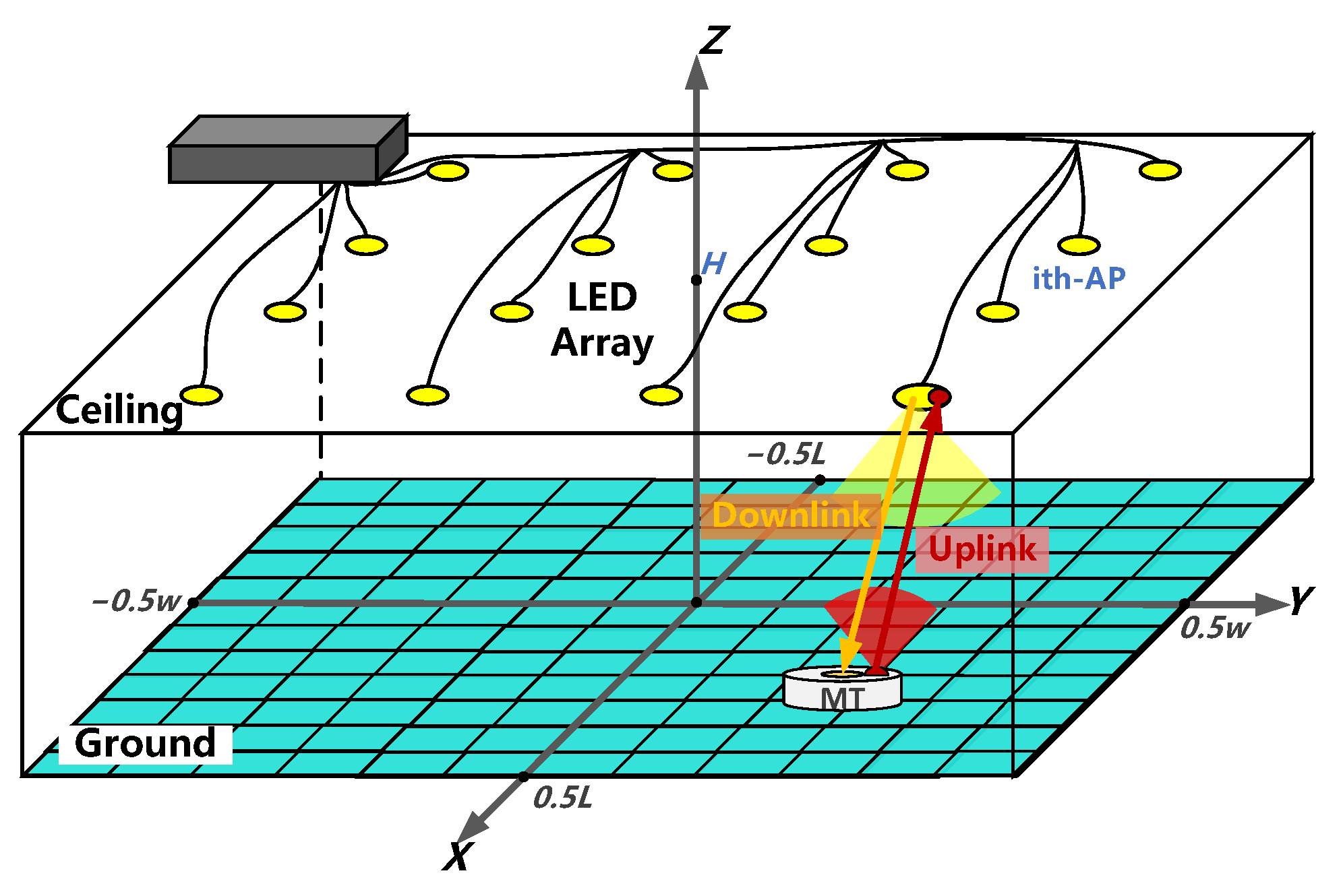
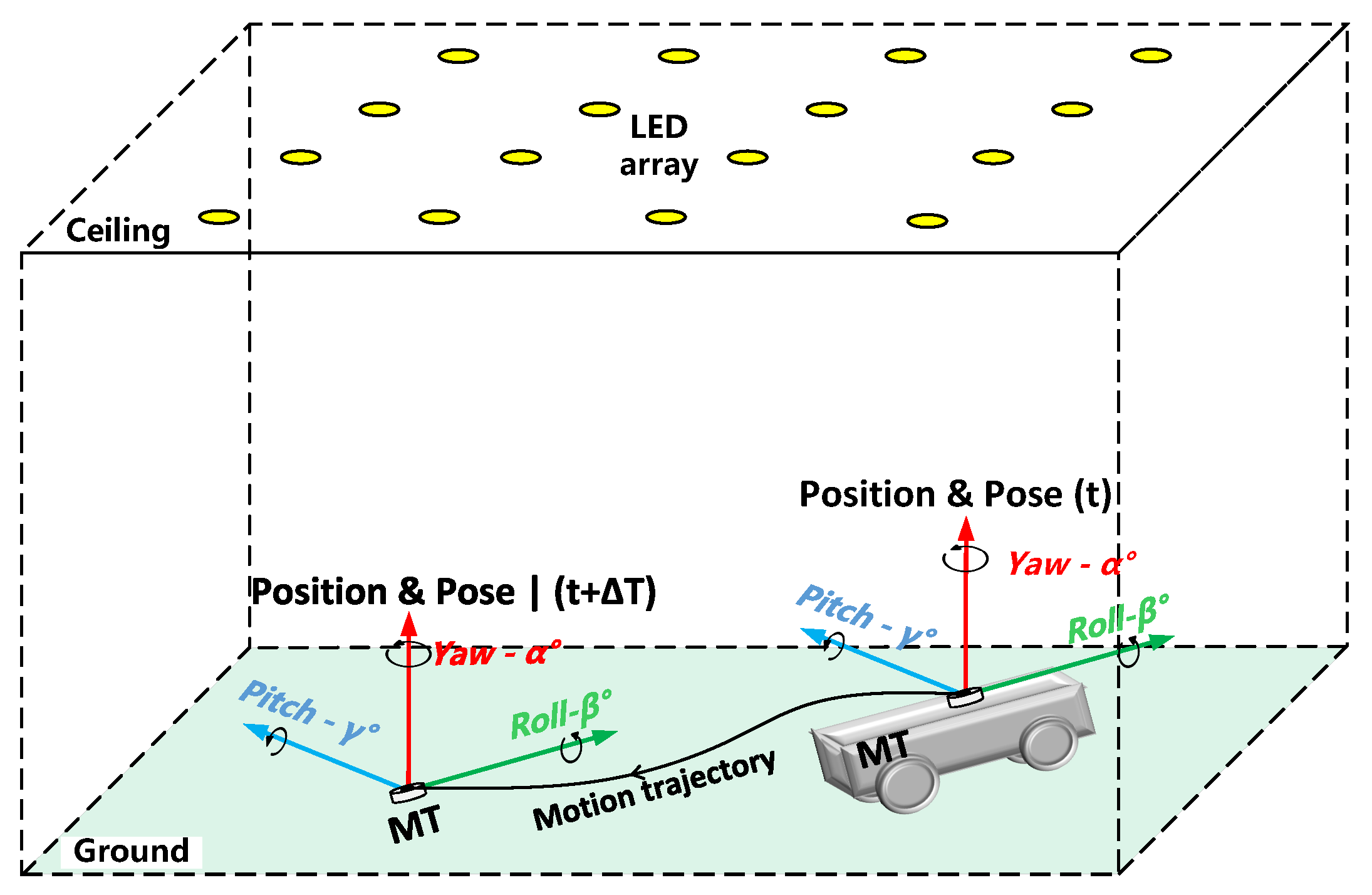
Figure 1 illustrates an indoor VLP system within a space of dimensions $L\times W\times H$, featuring typical VLC links between Access Points (APs) and Mobile Terminals (MTs). The ceiling deploys $N_r$ visible light APs, each vertically oriented downward and integrated with paired LED and PD modules. The floor level accommodates VLC-enabled MTs, each equipped with $N_t$ Infrared LEDs and $N_t$ PDs for uplink transmission and downlink reception, respectively. Utilizing distinct optical spectra for uplink (${\lambda }_{\mathrm{IR}}$) and downlink (${\lambda }_{\mathrm{vis}}$) cross-interference is avoided, thereby enabling full-duplex communication.

2.2. Target Motion Model

(1) Target motion state: In indoor environments, the target is assumed to follow regular motion patterns. Considering the movement characteristics of AGVs or robots, the target’s motion state can be described using deterministic and stochastic components. Let the uniform motion velocity be $u_R\in {\mathbb{R}}^3$, where $|u_R{|}_2=v_u$ m/s and $v_u\in {\mathbb{R}}^{+}$ denotes the speed magnitude. The random motion vector at time t, $v_R^{\left(t\right)}\in {\mathbb{R}}^3$, follows a Gaussian random process, i.e., $v_R^{\left(t\right)}\sim \mathcal{N}(0,V_s)$, where $V_s\in {\mathbb{R}}^{3\times 3}$ is the covariance matrix. The target’s position and orientation are assumed to be constrained by motion control, as shown in Figure 2. Under these assumptions, the discrete-time position evolution equation of the target is expressed as Equation (1):

$$x_R^{(t+1)}=x_R^{\left(t\right)}+\Delta t\times v_R^{\left(t\right)}$$

(1)

where $\Delta t$ is the sampling time interval. This model focuses on predictable regular motion characteristics, provides kinematic prior constraints for the dynamic positioning algorithm.

(2) Target position and orientation distribution: The spatial orientation of the MT is represented by three Euler angles: $\alpha$, $\beta$, and $\gamma$, corresponding to yaw, pitch, and roll around the Z-, X-, and Y-axes, respectively. Specifically, $\alpha \in [0^{\circ },{360}^{\circ })$, $\beta \in [-{180}^{\circ },{180}^{\circ })$, and $\gamma \in [-{90}^{\circ },{90}^{\circ })$.

According to Euler’s rotation theorem, any rotation matrix can be expressed as $\mathbf{R}={\mathbf{R}}_{\alpha }{\mathbf{R}}_{\beta }{\mathbf{R}}_{\gamma }$. This rotational transformation directly affects path angle calculations, which in turn influence the received light intensity and ultimately the RSS features and positioning results. Therefore, accurate modeling of orientation angles is essential for achieving high-precision 6D positioning.

2.3. Signal Analysis

(1) Channel gain: As depicted in Figure 3, the channel gain matrix $\mathbf{H}$ is defined in [20]. For $i\in [1,N_{\mathrm{r}}]$ and $j\in [1,N_{\mathrm{t}}]$, the channel matrix can be expressed as Equation (2):

$$\mathbf{H}=\left(\begin{array}{ccc}{h}_{1,1}& \dots & h_{1,N_t}\\ ⋮& \ddots & ⋮\\ h_{N_r,1}& \dots & h_{N_r,N_t}\end{array}\right)$$

(2)

Each element of the matrix can be further decomposed into the Line-of-Sight (LOS) gain $h_{i,j}^{\mathrm{LOS}}$ and Non-Line-of-Sight (NLOS) gain $h_{i,j}^{\mathrm{NLOS}}$, expressed as Equation (3):

$$h_{i,j}=h_{i,j}^{\mathrm{LOS}}+h_{i,j}^{\mathrm{NLOS}}$$

(3)

According to [21], the LOS channel gain $h_{i,j}^{\mathrm{LOS}}$ is given by Equation (4):

$$\begin{array}{cc}\hfill h_{i,j}^{\mathrm{LOS}}=& {\displaystyle \frac{(m+1)A}{2\pi d_{i,j}^2}}{cos}^m\left({\varphi }_{i,j}\right)\mathrm{rect}\left({\displaystyle \frac{{\varphi }_{i,j}}{\mathrm{\Phi }}}\right)\hfill \\ \hfill & \times cos\left({\psi }_{i,j}\right)\mathrm{rect}\left({\displaystyle \frac{{\psi }_{i,j}}{\mathrm{\Psi }}}\right)\hfill \end{array}$$

(4)

where ${\varphi }_{i,j}$ is the radiation angle, Φ is the field of view (FOV), ${\psi }_{i,j}$ is the incident angle, and Ψ is the FOV of the PD at the light source. $d_{i,j}$ represents the distance between the transmitter and receiver. The parameter $m=-1/{log}_2\left(cos\left({\mathrm{\Phi }}_{1/2}\right)\right)$ denotes the Lambertian emission order of the IR-LED.

To estimate the NLOS channel gain $h_{i,j}^{\mathrm{NLOS}}$, we use the multi-reflection modeling method described in [22]. This method divides the indoor environment into several surface elements with diffuse reflection characteristics, each treated as a Lambertian radiator. The entire indoor space is assumed to be divided into K reflective units, with each reflective surface acting as a secondary signal source, enabling multiple reflections modeling. The NLOS channel gain $h_{i,j}^{\mathrm{NLOS}}$ is then expressed as Equation (5):

$$h_{i,j}^{\mathrm{NLOS}}={\mathbf{r}}^{\mathrm{T}}{\mathbf{G}}_{\zeta }{\left(\mathbf{I}-\mathbf{E}{\mathbf{G}}_{\zeta }\right)}^{-1}\mathbf{t}$$

(5)

where vectors $\mathbf{t}$ and $\mathbf{r}$ represent the LOS links between the j-th IR-LED and all surface elements in the room, and from all surface elements in the room to the i-th AP [22], respectively. The matrix ${\mathbf{G}}_{\zeta }=diag({\zeta }_1,\dots ,{\zeta }_K)$ is the reflection coefficient matrix of all K reflectors, with E representing the $K\times K$ LOS transfer function matrix linking all surface units, and $I_K$ is the K-dimensional identity matrix. Thus, the channel matrix $\mathbf{H}$ has been derived, with all elements explicitly calculated via LOS and NLOS path modeling.

(2) Received signal analysis: The received optical power can be expressed as $\mathbf{P}\mathrm{r}=\mathbf{H}\mathbf{P}\mathrm{t}$. The PD responsivity is denoted by $R_{\mathrm{p}}$ (A/W), which converts the incident optical power to current. The signal is then amplified by a transimpedance amplifier with gain T (V/A), generating a voltage signal vector. The signal can be described as Equation (6):

$$\mathbf{y}=\lambda \mathbf{H}\mathbf{x}+\mathbf{n}$$

(6)

where $\lambda =T{R}_{\mathrm{P}}\eta$, and $\mathbf{n}={\left[n_1,n_2,\dots ,n_{N_{\mathrm{r}}}\right]}^T$ represents the $N_{\mathrm{r}}\times 1$ noise vector at the PD, which follows a real-valued additive Gaussian white noise distribution, $\mathcal{N}\left({\mathbf{0}}_{N_{\mathrm{r}}},{\sigma }_{\mathrm{n}}^2{\mathbf{I}}_{N_{\mathrm{r}}}\right)$, where ${\sigma }_{\mathrm{n}}^2=N_{0}B$, and B is the bandwidth.

Pose estimation requires broadcasting reference signals to all receiving APs. Assuming the received signal at the i-th AP is $y_i=\left(\lambda {\sum }_{j=1}^{N_{\mathrm{t}}}{h}_{i,j}\right)s+n_i$, the signal-to-noise ratio (SNR) can be expressed as Equation (7):

$${\rho }_i={\displaystyle \frac{{\left(\lambda {\sum }_{j=1}^{N_{\mathrm{t}}}{h}_{i,j}\right)}^2{P}_{\mathrm{elec}}}{{\sigma }_n^2}}$$

(7)

The received signals at any given communication time can be represented as a vector $\rho$, determined by the channel matrix $\mathbf{H}$, which is a function of the MT’s 6-DoF pose parameters $(x,y,z,\alpha ,\beta ,\gamma )$. The coordinates $(x,y,z)$ represent the instantaneous spatial position of the MT, while $(\alpha ,\beta ,\gamma )$ reflect its instantaneous orientation. This mapping indicates that the instantaneous received signal features can uniquely reconstruct the position and orientation of the MT at any given time.

Further considering dynamic continuity: In practical positioning scenarios, the received signals of the MT are continuously sampled over time. The resulting RSS time series essentially represents the projection of the target’s motion trajectory in signal strength space, with inherent spatiotemporal correlations encoding the target’s kinematic characteristics. This leads to the core principle of dynamic estimation: In the instantaneous dimension, the received signal strength(RSS) at a single moment contains the static pose information of the MT at that time; in the temporal dimension, the continuous sequence of received signals forms a dynamic observation signal $S_{1:T}$, where its temporal evolution directly represents the complete motion trajectory of the MT over the observation period. In other words, the instantaneous signal strength provides the current position and orientation, while the time-series data reveals the motion patterns and trajectory changes of the target, together supporting dynamic positioning and pose estimation of the target.

2.4. Data Generation

To build a dataset that links RSS measurements with position and orientation labels for training a subsequent model, we generate the dataset using the following steps:

(1) Generation of position samples: Based on the statistical distribution assumptions in [23], the position of the MT follows a uniform distribution in the spatial domain, given by Equation (8):

$$\begin{array}{cccc}\hfill & f_x\left(x\right)={\displaystyle \frac{1}{L}}{\mathcal{U}}_{\left[-{\displaystyle \frac{L}{2}},{\displaystyle \frac{L}{2}}\right]}\left(x\right),\hfill & \hfill f_y\left(y\right)={\displaystyle \frac{1}{W}}{\mathcal{U}}_{\left[-{\displaystyle \frac{W}{2}},{\displaystyle \frac{W}{2}}\right]}\left(y\right),& f_z\left(z\right)={\displaystyle \frac{1}{H_{\mathrm{device}}}}{\mathcal{U}}_{\left[0,H_{\mathrm{device}}\right]}\left(z\right)\hfill \end{array}$$

(8)

where $H_{\mathrm{device}}$ represents the maximum height of the MT, and $f_X\left(·\right)$ is the probability density function of the random variable X.

(2) Generation of orientation angle samples: According to the statistical model for accurate measurement of rotational angles provided in [24], we assume that the orientation angles follow a truncated Laplace distribution in space. The mean and standard deviation are as follows Equation (9):

$$\begin{array}{c}\left({\mu }_{\alpha },{\sigma }_{\alpha }\right)=\left(\mathrm{\Omega }-{90}^{\circ },3.{67}^{\circ }\right),\left({\mu }_{\beta },{\sigma }_{\beta }\right)=\left(40.{78}^{\circ },2.{39}^{\circ }\right),\left({\mu }_{\gamma },{\sigma }_{\gamma }\right)=\left(-0.{84}^{\circ },2.{21}^{\circ }\right)\end{array}$$

(9)

where Ω denotes the movement direction measured from the east direction of the Earth coordinate system, which follows a uniform distribution within the range of $[0^{\circ },{360}^{\circ }]$.

(3) Computation of corresponding SNR vectors: After generating the spatial samples, we calculate the channel matrix $\mathbf{H}$ for each position and orientation based on the previously outlined received signal model. The corresponding received SNR vector, $\rho$, is then computed. Finally, the feature vector is stored in the dataset RSS_total.mat, and the corresponding labels are stored in Label.mat.

3. Proposed Method

3.1. Overall Architecture Design

3.1.1. Spatiotemporal Correlation of Observation Samples

As discussed in Section 2.3, the temporal sequence of the received signals is intrinsically linked to the dynamic pose state of the moving target. Both of these are jointly involved in the foundation of positioning observations through the spatiotemporal coupling mechanism.

(1) Spatial dimensional correlation: The RSS signal is essentially the geometric projection of the light signal onto the PD array. Based on the Lambert radiation model, the time-varying RSS between the i-th LED and the j-th PD can be modeled as Equation (10):

$$s_{ij}\left(t\right)={\displaystyle \frac{(m+1)A}{2\pi d_{ij}^2\left(t\right)}}{P}_t{cos}^m\left({\varphi }_{ij}\left(t\right)\right)cos\left({\theta }_{ij}\left(t\right)\right)·T_s\left({\theta }_{ij}\left(t\right)\right)·g\left({\theta }_{ij}\left(t\right)\right)$$

(10)

Here, $d_{ij}\left(t\right)$ represents the time-varying transmission distance. The target’s pose determines the spatial distribution of the RSS through two mechanisms:

Position-to-signal mapping: The target’s position and orientation directly determine the transmission distance $d_{ij}\left(t\right)$. According to the inverse square law, changes in pose induce alterations in the RSS spatial gradient as Equation (11):

$${\displaystyle \frac{\partial s_{ij}}{\partial \mathbf{p}}}\propto -{\displaystyle \frac{2}{d_{ij}^3}}{\displaystyle \frac{\partial d_{ij}}{\partial \mathbf{p}}}$$

(11)

Orientation-to-signal mapping: Changes in orientation affect the receiving angle ${\theta }_{ij}$ through adjustments to the PD normal vector ${\mathbf{n}}_{P{D}_j}$ in Equation (12):

$$cos\left({\theta }_{ij}\left(t\right)\right)={\mathbf{n}}_{P{D}_j}(\alpha \left(t\right),\beta \left(t\right),\gamma \left(t\right))·{\displaystyle \frac{{\mathbf{p}}_{LE{D}_i}-{\mathbf{p}}_{P{D}_j}\left(t\right)}{∥{\mathbf{p}}_{LE{D}_i}-{\mathbf{p}}_{P{D}_j}\left(t\right)∥}}$$

(12)

Thus, the spatial distribution of the RSS signal can be decoupled as a geometric function of the pose parameters, embedding the mapping information between target pose and signal geometry.

(2) Temporal dimensional correlation: The RSS sequence evolves under the constraint of the target’s motion continuity. It is inherently the projection of the target’s motion trajectory in the signal strength space. The continuous sequence of received signals forms the dynamic observation series $S_{1:T}$, where the temporal evolution directly represents the complete motion trajectory of the target during the observation period. Assuming that the target’s pose change within a short time interval $\Delta t$ satisfies the continuity assumption as Equation (13):

$$\mathbf{P}(t+\Delta t)=\mathbf{P}\left(t\right)+\mathbf{v}\left(t\right)\Delta t+\mathcal{O}\left(\Delta t^2\right)$$

(13)

This equation describes the state change of the target between time t and $t+\Delta t$. The target’s current position, orientation, velocity, and the time interval jointly determine its subsequent state. This dependency allows temporal convolutions to effectively model the sequential evolution of the pose trajectory.

3.1.2. Algorithm Framework

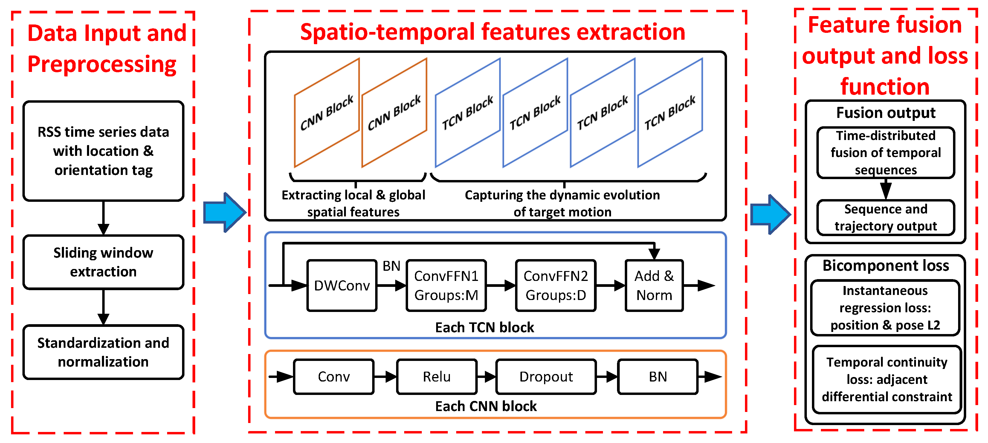
To overcome the accuracy degradation problem in dynamic positioning due to the insufficient consideration of spatiotemporal dependencies in traditional methods, we propose the STFI-Net. This method utilizes the inherent spatiotemporal dependencies within the RSS temporal sequence. Following the design principle of “spatial geometry feature extraction → temporal pattern modeling → spatiotemporal feature fusion,” the overall architecture of the proposed solution is shown in Figure 4.

3.1.3. Novelty Analysis Relative to Traditional Methods

To clarify the fundamental novelty of STFI-Net relative to traditional CNN/LSTM and quasi-recurrent network (QRN) approaches, we provide a comprehensive analysis across multiple dimensions that demonstrates the radical departure our method represents from existing temporal modeling paradigms in

Table 1. Temporal modeling method comparison analysis.

Dimension	CNN+LSTM	Quasi-Recurrent Networks (QRN)	STFI-Net (CNN+Modern TCN)
Architecture	Sequential processing, hidden state propagation	Convolution-recurrent hybrid	Pure convolution, fully parallel
Temporal Dependency	Black-box hidden state learning	Partial explicit modeling	Explicit decoupling of three dependencies
Receptive Field	Fixed gating mechanism	Fixed convolution kernels	Multi-scale large kernels + dilation
VLP Adaptation	Generic time series method	Generic time series method	RSS signal-specific optimization
Parallelization	Low (sequential constraint)	Medium	High (fully parallel)
Gradient Stability	Vanishing gradient problem	Partially improved	Residual + BN complete solution
Computational Complexity	$O\left(T·H^2\right)$	$O\left(T·K·H\right)$	$O\left(T·K·H\right)$, K parallelizable
Sequence Output	Requires additional design	Requires additional design	Native sequence-to-sequence support
Training Efficiency	Baseline	1.5–2× improvement	3–5× improvement

. Unlike CNN+LSTM approaches that rely on opaque hidden states to capture temporal patterns through sequential processing and state propagation, and QRNs that provide only partial explicit modeling via convolution–recurrent hybrid architectures, STFI-Net decomposes complex temporal dependencies into three orthogonal and interpretable components. This explicit decomposition encompasses: (1) single-variable temporal dependency captured through depthwise separable convolutions that model the intrinsic continuity within each RSS signal sequence, (2) intra-channel dependency modeled through grouped convolutions that capture feature interactions within individual spatial dimensions, and (3) cross-variable dependency learned via cross-variable feed-forward networks that enable information fusion across the entire RSS signal space.

The architectural innovations of STFI-Net extend beyond temporal dependency modeling to encompass fundamental improvements in receptive field design and computational efficiency. While traditional CNN+LSTM methods employ fixed gating mechanisms that limit their ability to capture varying temporal scales, and QRN approaches utilize fixed convolution kernels that constrain their temporal modeling capacity, STFI-Net introduces multi-scale dilated convolutions with large kernel designs (15, 31, 63) specifically optimized for capturing the heterogeneous temporal characteristics of target motion in indoor environments. This multi-scale approach enables the network to simultaneously model short-term signal fluctuations and long-term trajectory patterns that are critical for accurate dynamic positioning.

Furthermore, STFI-Net incorporates RSS signal-specific optimizations that are fundamentally absent from generic temporal modeling approaches employed by CNN+LSTM and QRN methods. These optimizations include a signal-aware kernel design that accounts for the unique propagation characteristics of optical signals in VLP systems, and motion pattern-specific architectural choices that leverage the geometric constraints inherent to indoor positioning scenarios. The pure convolutional architecture eliminates the gradient instability problems that plague recurrent structures, achieving three to five times training efficiency improvements over conventional methods while maintaining complete parallelization capabilities that enable real-time deployment in resource-constrained environments.

3.2. Input Data Preprocessing

To ensure effective network training, the input data need two essential preprocessing steps: time window segmentation and sequence construction, followed by data standardization. These operations transform the original RSS signals into a format suitable for deep learning models, thereby enhancing the extraction of spatiotemporal features associated with target motion.

3.2.1. Time-Window Segmentation and Sequence Construction

Traditional static positioning methods typically process RSS observation vectors from individual time instances. However, in dynamic positioning scenarios, it is crucial to incorporate temporal dependencies to capture continuous variations in target position and orientation. To this end, this study employs a sliding time window strategy to organize the continuous RSS observation sequence, leveraging temporal dependencies to learn the dynamic motion trajectory of the target.

Raw Data Sequence: The continuous RSS observation sequence at different time instants is defined as Equation (14):

$$\mathbf{X}=\left\{{\mathbf{x}}_1,{\mathbf{x}}_2,\dots ,{\mathbf{x}}_N\right\},{\mathbf{x}}_{\tau }\in {\mathbb{R}}^{16}$$

(14)

where N is the total number of sampling points, and ${\mathbf{x}}_{\tau }={[s_1\left(\tau \right),s_2\left(\tau \right),\dots ,s_{16}\left(\tau \right)]}^T$ represents the RSS signal strengths of the APs at the $\tau$-th time instant.

Sliding window construction: To convert the continuous RSS sequence into a temporal data sample suitable for the model, a fixed-length sliding window is used. Each time window contains a continuous RSS subsequence of length T, defined as Equation (15):

$${\mathbf{W}}_t=\left\{{\mathbf{x}}_{\tau }\mid \tau \in [t-T+1,t]\right\}=\left[{\mathbf{x}}_{t-T+1},{\mathbf{x}}_{t-T+2},\dots ,{\mathbf{x}}_t\right]$$

(15)

where T is Window length, determined by the target’s velocity v and the sampling rate $f_s$; s represents sliding step size, controlling the overlap between adjacent windows, with $s\in [1,T/2]$; $f_s$ is sampling frequency, ensuring the time resolution meets the target’s motion capture requirements.

Window generation: Training samples are generated by sliding the window with step size s in Equation (16):

$$\mathcal{W}=\left\{{\mathbf{W}}_{t_i}\mid t_i=T+(i-1)·s,i=1,2,\dots ,M\right\}$$

(16)

where $M=\lfloor (N-T)/s\rfloor +1$ represents the total number of windows generated.

Three-dimensional tensor organization: To meet the input requirements of the deep learning framework, each time-window sequence is reorganized into a three-dimensional tensor as Equation (17):

$${\mathbf{X}}^{\left(\mathrm{batch}\right)}\in {\mathbb{R}}^{B\times T\times 16}$$

(17)

where, B: Batch size indicating the number of samples in a training batch; T is time window length.

3.2.2. Data Normalization

Differences in the transmit power, installation position, and optical characteristics of different APs lead to significant scale variations in the raw RSS signals, which can adversely affect the convergence and stability of network training. Therefore, RSS signals undergo standardization to eliminate these scale differences across APs. Each AP’s RSS signal is normalized to have zero mean and unit variance, as defined by Equation (18):

$$\tilde{x}(\tau ,i)={\displaystyle \frac{x(\tau ,i)-{\mu }_i}{{\sigma }_i}}$$

(18)

where $x(\tau ,i)$ is the raw RSS value of the i-th AP at the $\tau$-th time instant; ${\mu }_i={\displaystyle \frac{1}{N}}{\sum }_{\tau =1}^{N}x(\tau ,i)$ is the sample mean; ${\sigma }_i=\sqrt{{\displaystyle \frac{1}{N-1}}{\sum }_{\tau =1}^N{(x(\tau ,i)-{\mu }_i)}^2}$ is the sample standard deviation.

3.3. Spatial Feature Extraction Module

The spatial feature extraction module serves to distill geometric-semantic features from single-frame RSS signals, thereby providing high-quality input representations for subsequent temporal modeling. A single-frame RSS measurement constitutes a spatially distributed signal representation, where each component corresponds to the response intensity of the i-th PD at time instance t, encapsulating rich geometric-semantic information pertaining to the target relative to the LED array. Disparities in signal intensity among adjacent PDs reflect the spatial gradient distribution of light intensity, whereas the aggregate signal distribution pattern across the PD array encodes the overarching geometric relationship between the target and the LED array.

To satisfy the real-time operational and computational efficiency demands inherent to dynamic positioning, this module adopts a lightweight two-layer convolutional architecture, structured as follows:

• First Layer (Local Feature Extraction): Employs a convolutional kernel of size $k_1=5$ alongside 64 filters to extract localized gradient features from the RSS signal, concentrating on short-range variations in signal intensity patterns.
• Second Layer (Global Semantic Encoding): Utilizes a convolutional kernel of size $k_2=3$ with 128 filters to broaden the receptive field, thereby amalgamating local features and deriving semantic features that characterize global distribution patterns and geometric relationships.

Each convolutional layer operates upon the input signal via localized receptive fields to extract spatial features, effectively capturing the signal’s geometric distribution and path loss characteristics. The corresponding operation is defined as Equation (19):

$${\mathbf{F}}_i=ReLU\left(\mathrm{BN}\left({\mathbf{W}}_i\ast {\mathbf{F}}_{i-1}+{\mathbf{b}}_i\right)\right)$$

(19)

where ${\mathbf{W}}_i$ denotes the convolutional kernel weights of the i-th layer, ∗ signifies the convolution operation, BN represents batch normalization, and ReLU is the rectified linear unit activation function. A dropout regularization with a rate of $0.2$ is applied subsequent to the first convolutional layer to mitigate overfitting. The resultant output feature vector is subsequently flattened and propagated as input to the ensuing network layers.

This module effectively transmutes the raw RSS time-series data into a compact semantic feature sequence denoted by ${\mathbf{Z}}^{\left(s\right)}\in {\mathbb{R}}^{B\times T\times D}$ (with $D=128$). This synthesized sequence integrates localized signal intensity information with global geometric contextual cues, substantially bolstering the model’s adaptability to dynamically moving targets. Through the collaborative extraction of local gradient variations and global geometric structures, the convolutional layers empower the module to: (i) discern relative geometric relationships between the target and the LED array; (ii) encode spatial attenuation characteristics inherent to optical signal propagation; and (iii) supply robust spatial prior knowledge essential for subsequent temporal modeling.

3.4. Time Series Modeling Module

The temporal modeling module employs a Modern-TCN architecture, designed to efficiently capture the dynamic evolution patterns of target motion from spatial feature sequences. In contrast to traditional sequential models (e.g., RNNs or LSTMs), the Modern TCN offers three distinct advantages inherent to its purely convolutional design: (i) parallel computation: the inherent parallelism of convolutional operations significantly accelerates the training process; (ii) long-range dependency modeling: dilated convolutions and large kernel sizes facilitate the capture of long-range temporal dependencies; (iii) training stability: the architecture circumvents the vanishing and exploding gradient problems prevalent in recurrent neural networks. This module innovatively decouples complex spatiotemporal dependencies into three orthogonal subtasks. A dedicated component is designed to model each specific dependency: temporal, intra-channel, and cross-variable.

Component 1: Depthwise separable convolution (DWConv)

This component independently learns the temporal dependencies within each variable sequence, capturing the intrinsic continuity and smoothness of the target’s motion. It is mathematically represented as Equation (20):

$${\mathbf{H}}_1=DWConv(\mathbf{X},K),\hspace{1em}\mathrm{group}=M\times D_{\mathrm{unit}}$$

(20)

Implementation steps: (i) Tensor reshaping: $\mathbf{X}\in {\mathbb{R}}^{B\times T\times M\times D_{\mathrm{unit}}}\to {\mathbb{R}}^{B\times T\times \left(M·D_{\mathrm{unit}}\right)}$ (ii) Depthwise convolution: Apply large kernel one-dimensional convolutions along the temporal dimension. (iii) Multi-scale perception: The convolution kernel size $K\in 15,31,63$, and dilation rate $d\in 1,2,4,8$.

Component 2: Channel-Wise feed-forward network (ConvFFN1)—Intra-channel dependency

This component learns dependencies between feature dimensions within each individual variable, enhancing representational capacity. It is primarily responsible for capturing short-term motion trajectories. The transformation is defined as Equation (21):

$${\mathbf{H}}_2=ConvFFN1\left({\mathbf{H}}_1\right),\hspace{1em}\mathrm{group}=M$$

(21)

The layer implements an expansion-reduction transformation: $D_{\mathrm{unit}}\to 4\times D_{\mathrm{unit}}\to D_{\mathrm{unit}}$.

Component 3: Cross-variable feed-forward network (ConvFFN2)—Cross-variable dependency

This component progressively fuses spatiotemporal semantic information to learn long-term behavioral patterns. The operation is defined as Equation (22):

$${\mathbf{H}}_3=ConvFFN2\left({\mathbf{H}}_2\right),\hspace{1em}\mathrm{group}=D_{\mathrm{unit}}$$

(22)

where grouped convolutions (group = $D_{\mathrm{unit}}$) enable efficient integration of multi-variable information. By decomposing temporal modeling into temporal, intra-channel, and cross-variable dependencies, the proposed module effectively balances local continuity, feature expressiveness, and global fusion, thereby providing a robust foundation for accurate and stable dynamic VLP.

3.5. Spatiotemporal Feature Fusion Strategy

The temporal features extracted by the Modern TCN are transformed into a compact global representation suitable for final pose estimation. To effectively fuse the spatiotemporal features and precisely represent the target’s dynamic evolution in both spatial and temporal domains, a dedicated output layer is designed. This layer comprises two TimeDistributed fully connected (FC) layers, which collectively enable the processing of sequential data and facilitate dynamic regression. The architecture is formulated as follows Equations (23) and (24):

Feature Transformation Layer:

$$\mathbf{H}=\mathrm{TimeDistributed}\left(ReLU\left({\mathbf{W}}_1{\mathbf{Z}}^{\left(st\right)}+{\mathbf{b}}_1\right)\right)$$

(23)

Pose Regression Layer:

$$\widehat{\mathbf{Y}}=\mathrm{TimeDistributed}\left({\mathbf{W}}_2\mathbf{H}+{\mathbf{b}}_2\right)$$

(24)

where ${\mathbf{W}}_1\in {\mathbb{R}}^{128\times 64}$ and ${\mathbf{W}}_2\in {\mathbb{R}}^{64\times 6}$ are the weight matrices of the respective FC layers. This hierarchical output architecture allows the model to effectively learn the complex nonlinear mapping from the 128-dimensional spatiotemporal features to the final 6-DoF pose estimates through an intermediate nonlinear transformation.

3.6. Joint Loss Function Design

For dynamic positioning tasks, the design of the loss function must simultaneously address two essential objectives: (i) Instantaneous accuracy, which ensures precise regression of the pose at each individual timestep, and (ii) Temporal continuity, which maintains the smoothness of the predicted trajectory by avoiding abrupt changes between consecutive frames. Therefore, we design a dual-component joint loss function that includes both the pose regression loss and the temporal continuity loss, which ensures accurate predictions at each time step while also guaranteeing the smooth variation in dynamic trajectories. The total loss function is given as Equation (25):

$${\mathcal{L}}_{\mathrm{total}}={\mathcal{L}}_{\mathrm{pose}}+{\lambda }_{\mathrm{temp}}{\mathcal{L}}_{\mathrm{temporal}}$$

(25)

where ${\mathcal{L}}_{\mathrm{pose}}$ is the pose regression loss, ${\mathcal{L}}_{\mathrm{temporal}}$ is the temporal continuity loss, ${\lambda }_{\mathrm{temp}}$ is the weight for the temporal loss, controlling the balance between pose regression loss and temporal continuity loss.

Pose regression loss: The pose regression loss is used to regress the error of the target’s position and orientation at each frame. It calculates the L2 regression errors for both position and orientation. The pose regression loss is defined as Equation (26):

$${\mathcal{L}}_{\mathrm{pose}}={∥{\mathbf{p}}_{\mathrm{pred}}-{\mathbf{p}}_{\mathrm{true}}∥}_2^2+{\lambda }_{\mathrm{rot}}{∥{\mathit{\theta }}_{\mathrm{pred}}-{\mathit{\theta }}_{\mathrm{true}}∥}_2^2$$

(26)

Here, ${\mathbf{p}}_{\mathrm{pred}}$ and ${\mathbf{p}}_{\mathrm{true}}$ represent the predicted and true position vectors, respectively, ${\mathit{\theta }}_{\mathrm{pred}}$ and ${\mathit{\theta }}_{\mathrm{true}}$ represent the predicted and true orientation angles (yaw $\alpha$, pitch $\beta$, roll $\gamma$), ${\lambda }_{\mathrm{rot}}$ is a weight parameter that adjusts the relative importance of the position and orientation losses.

Temporal continuity loss: To ensure the smoothness and consistency of the time series, we introduce a temporal difference loss, which constrains the change between adjacent time steps. The temporal continuity loss is formulated as Equation (27):

$${\mathcal{L}}_{\mathrm{temporal}}=\sum _{t=2}^T{∥{\widehat{\mathbf{y}}}_t-{\widehat{\mathbf{y}}}_{t-1}∥}_2^2$$

(27)

where ${\widehat{\mathbf{y}}}_t=[{\widehat{\mathbf{p}}}_t;{\widehat{\mathit{\theta }}}_t]\in {\mathbb{R}}^6$ represents the predicted pose at time step t, including position ${\widehat{\mathbf{p}}}_t$ and orientation ${\widehat{\mathit{\theta }}}_t$, ${\left|\widehat{\mathbf{y}}t-\widehat{\mathbf{y}}t-1\right|}_2^2$ calculates the L2 difference between the predicted poses at consecutive time steps. This loss ensures the smoothness of the motion trajectory and improves the model’s ability to adapt to dynamic targets by penalizing large changes between consecutive frames.

Hyperparameter selection rationale: To ensure methodological rigor in loss function parameter selection, we conducted a comprehensive sensitivity analysis on key hyperparameters ${\lambda }_{rot}$ and ${\lambda }_{temp}$. Through systematic grid search over ${\lambda }_{rot}\in \{0.2,0.4,0.6,0.8,1.0,1.2,1.5,2.0\}$ and ${\lambda }_{temp}\in \{0.01,0.03,0.05,0.08,0.10,0.15,0.20,0.30\}$, we validated that our selected parameters (${\lambda }_{rot}=0.8$, ${\lambda }_{temp}\in [0.05,0.10,0.15]$) achieve optimal performance across multiple evaluation metrics. The analysis confirms that ${\lambda }_{rot}=0.8$ provides the best position–orientation trade-off, while the ${\lambda }_{temp}$ range [0.05–0.15] optimally balances trajectory smoothness and prediction accuracy under varying motion complexities. Detailed sensitivity analysis results are presented in Section 4.2.3.

4. Experimental Design and Analysis

This chapter employs an experimental methodology to evaluate the proposed approach. Section 4.1 elaborates on the experimental setup, encompassing the environment, simulation parameters, metrics. Section 4.2 and Section 4.3 present a comparative analysis validating the model’s performance against state-of-the-art schemes published within the last five years.

4.1. Experimental Setup

(1) Hardware and software configuration: All experiments were conducted on a uniform platform, with detailed specifications provided in

Table 2. Hardware/software configuration.

Hardware/Software	Version
CPU	Intel Xeon E5-2680 V3 ×2
GPU	NVIDIA TITAN X Pascal 12 GB
Memory	64 G
Development tool	Matlab2021/Python3.10/DataSpell 2021

. The implementation utilized a hybrid development environment incorporating MATLAB 2021, Python 3.10, and JetBrains DataSpell 2021.

(2) VLP system modeling parameters: The system configuration was designed to emulate realistic deployment conditions, representative of industrial or intelligent space applications. The comprehensive simulation and modeling parameters for the VLP-based system are summarized in

Table 3. VLP system modeling parameters.

Parameter	Symbol	Value
Room dimension	$L\times W\times H$	$(5\times 5\times 3) \mathrm{m}$
The number of AP (ceiling)	$N_r$	16
LED half-power semiangle	${\mathrm{\Phi }}_{1/2}$	${60}^{\circ }$
PD responsivity	$R_p$	$0.6 \mathrm{A}/\mathrm{W}$
Refractive index of concentrator	$n_c$	1
Maximum MT’s height	$H_{\mathrm{device}}$	$1.5 \mathrm{m}$
Maximum MT’s power	$P_{\mathrm{elec}}^{\max }$	$0.01\mathrm{W}$
Walls reflection	$\zeta$	0.7
PD FOV	$\mathrm{\Psi }$	${90}^{\circ }$
System bandwidth	B	$10 \mathrm{MHz}$
Noise power spectral density	$N_0$	${10}^{-21} \mathrm{W}/\mathrm{Hz}$

.

(3) Neural network parameters: The deep learning model, STFI-NET, was architected to process the acquired RSS data. The critical hyperparameters, including the learning rate, optimizer configuration, kernel dimensions, and training regimen, are explicitly provided in

Table 4. STFI-Net parameters configuration.

Category	Parameter	Value	Description
Data processing	Time window length T	20–40	Input sequence length
	Sliding step s	8	Window sliding stride
	Train/Test split	0.8/0.2	Dataset partition ratio
Network architecture	CNN layers	2	Spatial feature extraction
	CNN filters	[64, 128]	Feature map channels
	CNN kernels	[5, 3]	Convolution kernel sizes
	TCN layers K	4	Temporal modeling depth
	TCN kernels	[15, 31, 31, 63]	Multi-scale temporal kernels
	TCN dilations	[1, 2, 4, 8]	Temporal receptive field
Training strategy	Optimizer	AdamW	Adaptive optimizer
	Learning rate ${\alpha }_0$	$1\times {10}^{-3}$	Initial learning rate
	Batch size B	32	Training batch size
	Total epochs	150	Complete training cycles
Regularization	CNN dropout	0.2	Spatial regularization
	TCN dropout	0.1	Temporal regularization
	Output dropout	0.1	Regression regularization
Loss function	Rotation weight ${\lambda }_{rot}$	0.8	Orientation loss weight
	Temporal weight ${\lambda }_{temp}$	[0.05, 0.1, 0.15]	Temporal consistency weight
	Loss type	L2	Mean squared error

.

The STFI-Net training employs a fixed learning rate of $1\times {10}^{-3}$ maintained consistently across all 150 epochs. This configuration utilizes the AdamW optimizer with carefully tuned hyperparameters: weight decay of 0.01, momentum coefficients ${\beta }_1=0.9$ and ${\beta }_2=0.999$, and numerical stability parameter $ϵ=1\times {10}^{-8}$. AdamW’s decoupled weight decay mechanism provides superior regularization for deep TCN architectures while ensuring stable gradient propagation.

The network undergoes supervised training for 150 epochs with batch size of 32, utilizing a comprehensive regularization framework to prevent overfitting. A hierarchical dropout strategy is implemented with differentiated rates: 0.2 for the two-layer CNN feature extraction module (64 and 128 filters with kernel sizes [5, 3]), 0.1 for the four-layer TCN temporal modeling module, and 0.1 for the final regression output layer. This multi-tier approach provides adaptive regularization strength corresponding to each layer’s representational capacity. The training employs an 80/20 train–test split as specified in Table 4, with the training duration empirically validated to ensure convergence stability while maintaining generalization performance.

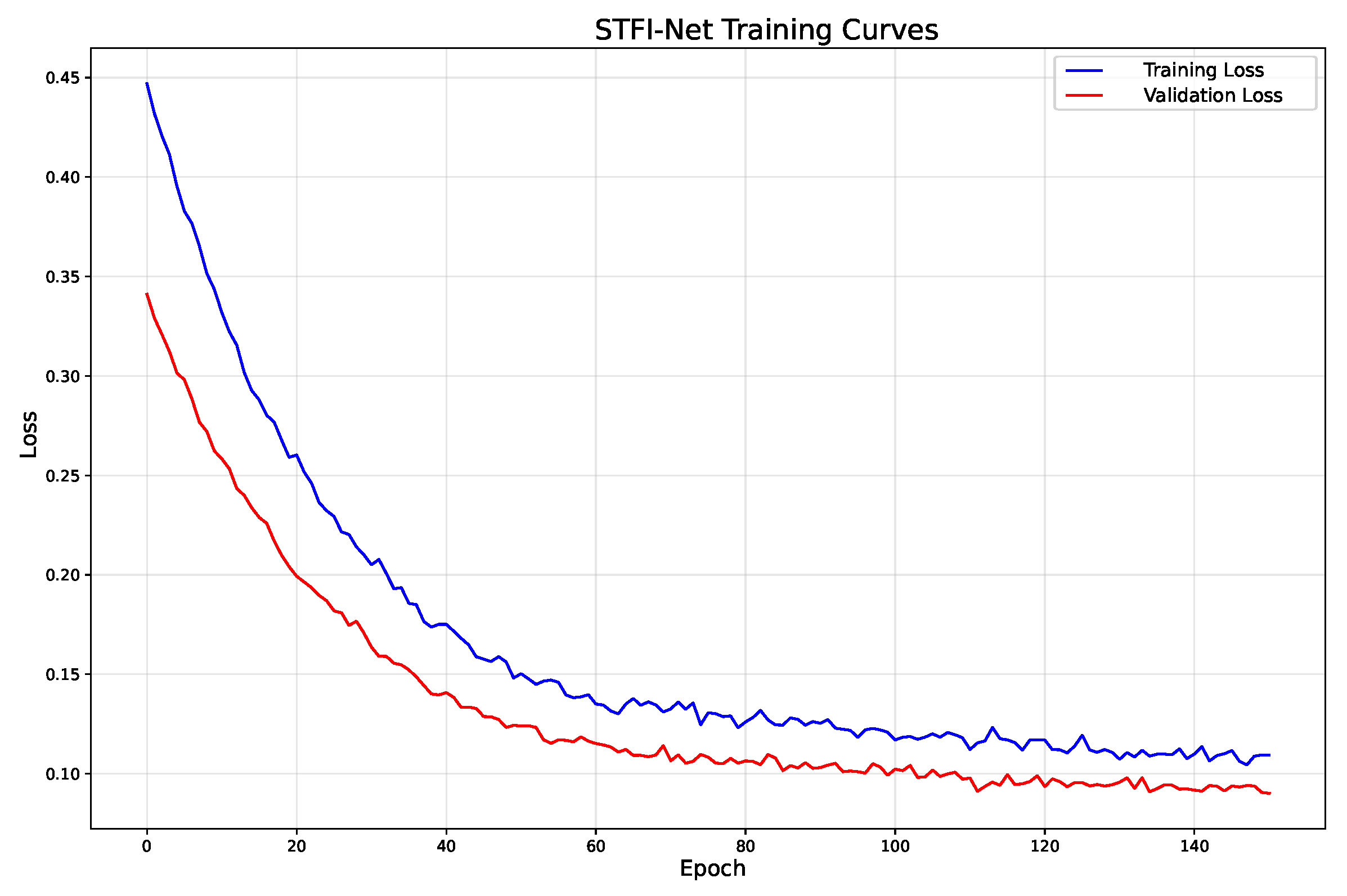
The training optimization employs a joint loss function with L2 regression, incorporating rotation weight ${\lambda }_{rot}=0.8$ and dynamic temporal weight ${\lambda }_{temp}\in [0.05, 0.1, 0.15]$ to balance position, orientation, and temporal consistency objectives. Figure 5 presents the loss evolution trajectories throughout the optimization process. The convergence profile exhibits several critical characteristics indicative of successful deep learning dynamics: (i) training loss consistently exceeds validation loss with a mean ratio of 1.21, demonstrating effective regularization without underfitting; (ii) monotonic loss reduction from initial values of 0.447 and 0.341 to final convergence at 0.109 and 0.090 for training and validation, respectively, corresponding to performance improvements of 75.5% and 73.6%; (iii) absence of gradient pathologies such as vanishing or exploding gradients, as evidenced by smooth, stable convergence without oscillatory behavior. The successful optimization to achieve a position estimation accuracy of 4.59 cm MAE validates both the architectural design and the efficacy of the training protocol for temporal VLP modeling applications.

(4) Evaluation metrics: To provide a thorough evaluation of the proposed model’s performance, the following metrics were utilized:

• MAE: Measures the average absolute deviation in position and orientation.
• RMSE: Quantifies the standard deviation of residuals in position and orientation.
• CDF curves: Analyze the distribution and stability of localization errors.
• Inference time: Represents the average latency per forward pass, indicating real-time inference capability.

4.2. Algorithm Performance

4.2.1. Static Estimation Error Analysis

To evaluate the estimation accuracy of the proposed model, we first examine its performance in estimating the 3D position and orientation using static points distributed within a three-dimensional space. Evaluation points were randomly sampled across multiple height planes (0.3 m, 0.6 m, 1.0 m, and 1.5 m).

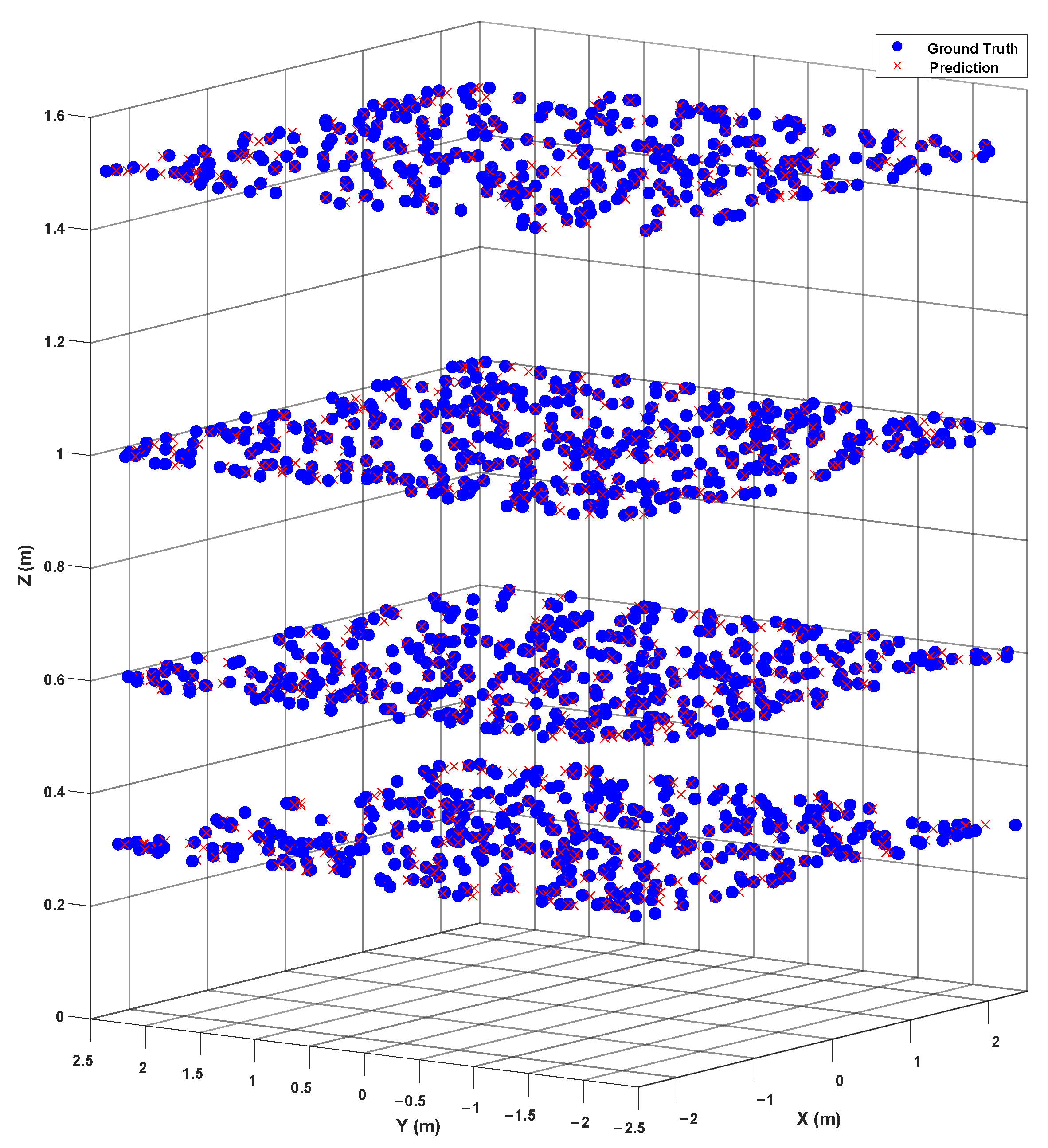
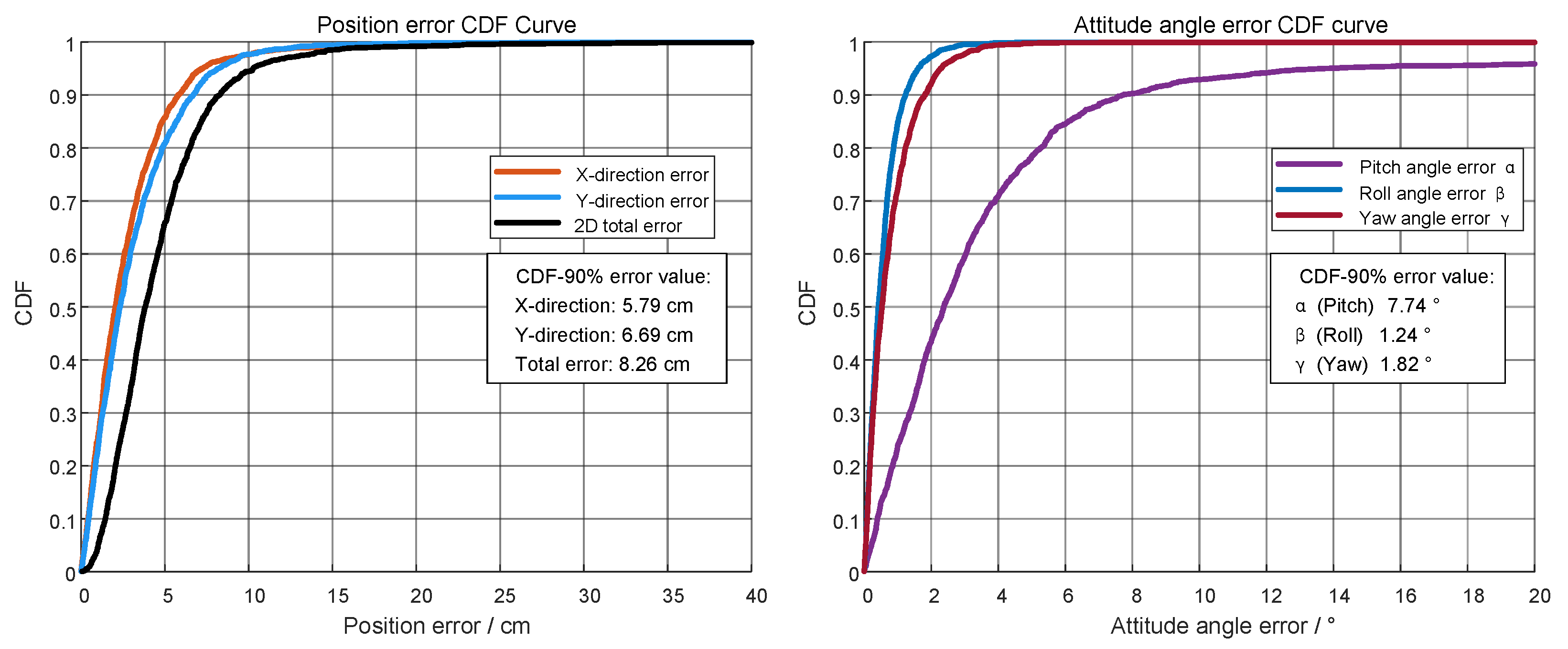
Figure 6 further complements the evaluation with 3D scatter plots that compare predicted and ground truth positions across various heights, providing a visual representation of the error distributions and estimation consistency per plane. As summarized in

Table 5. Spatial 3D position estimation error statistics.

Position	MAE (cm)	RMSE (cm)	CDF-90% Err. (cm)
x	2.78	4.05	5.79
y	3.06	4.14	6.69
total	4.59	5.79	8.26

, the mean absolute error (MAE), root mean square error (RMSE), and the 90th percentile error derived from the cumulative distribution function (CDF-90%) for 3D position estimation are 4.59 cm, 5.79 cm, and 8.26 cm, respectively. These results confirm the high accuracy of the proposed method in locating targets within a 3D environment. Orientation estimation errors, measured across yaw ($\alpha$), pitch ($\beta$), and roll ($\gamma$) angles, are detailed in

Table 6. Spatial 3D orientation estimation error statistics.

Attitude	MAE (°)	RMSE (°)	CDF-90% Err. (°)
$\alpha$	5.29	11.42	7.74
$\beta$	0.57	0.78	1.24
$\gamma$	0.76	1.10	1.82

. The yaw angle exhibits an MAE of 5.29°, RMSE of 11.42°, and CDF-90% error of 7.74°. In contrast, pitch and roll angles demonstrate significantly higher accuracy, with CDF-90% errors remaining within approximately 1°.

Additionally, Figure 7 presents CDF curves for both position and orientation errors, enabling a comprehensive assessment of localization robustness. Overall, the proposed model demonstrates high accuracy and robustness in estimating position and orientation within a static 3D space, exhibiting excellent performance across all height planes. To further validate its performance in dynamic tasks, the model is evaluated on trajectory estimation in the following subsection.

4.2.2. Dynamic Trajectory Error Analysis

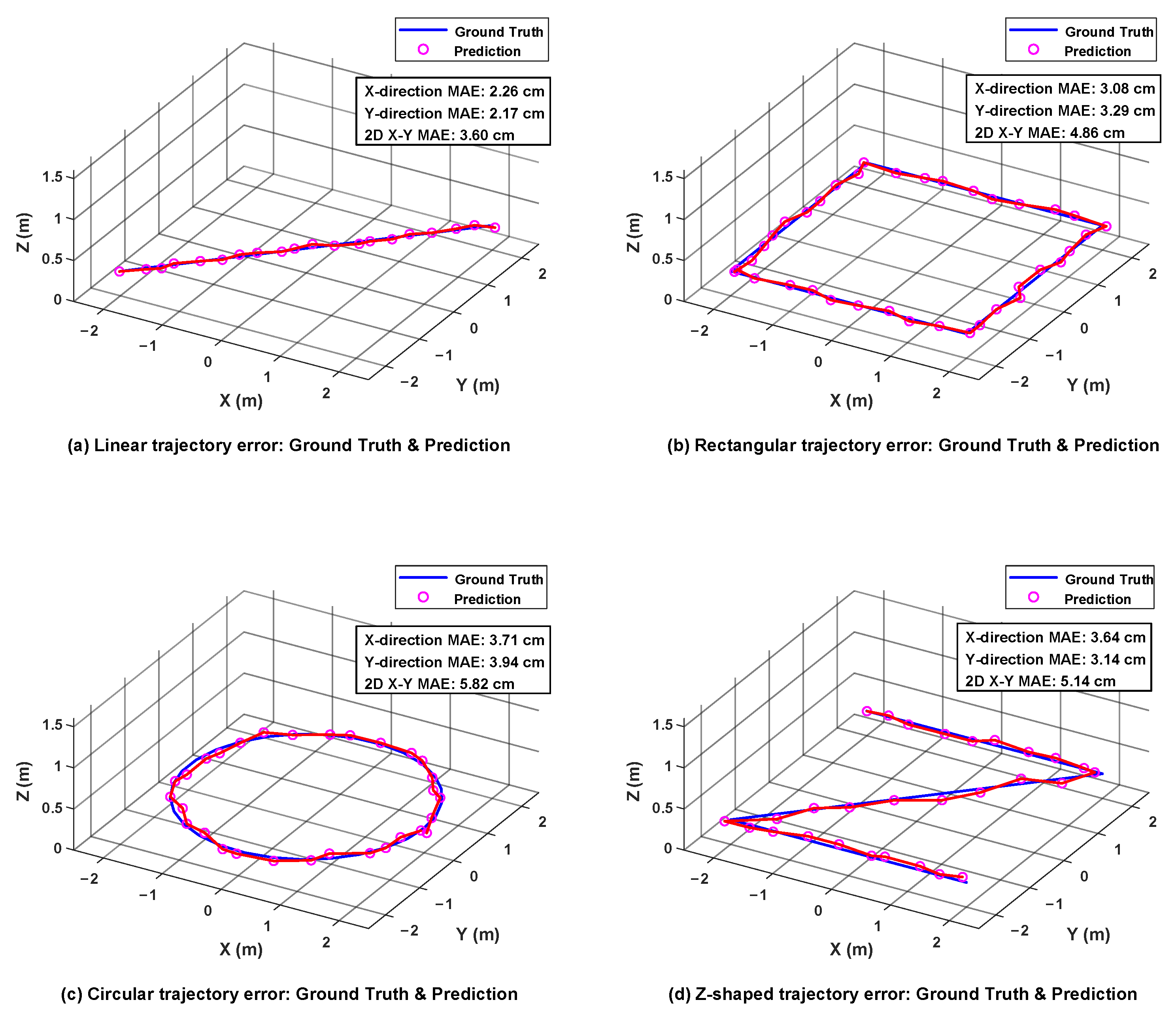
To evaluate the model’s dynamic performance, we conducted a comprehensive analysis of different trajectory estimation at a fixed height of 0.3 m, representing a typical height for AGV operational scenarios. Four distinct motion patterns (linear, rectangular, circular, and Z-shaped) were employed to assess spatial regression capability between predicted paths and ground truth measurements. Performance was quantified using MAE, RMSE, and CDF-90% metrics for both position and orientation estimation.

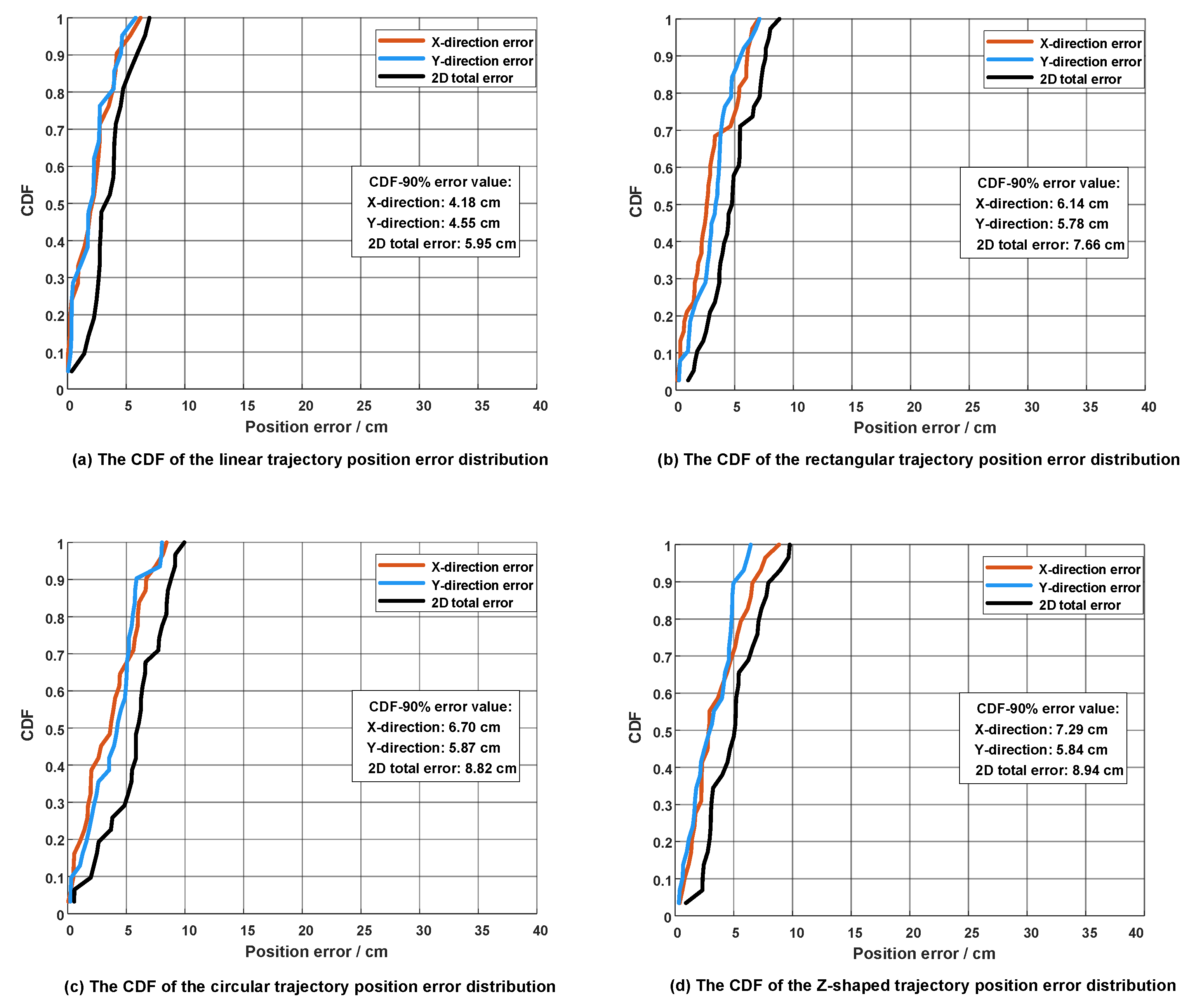
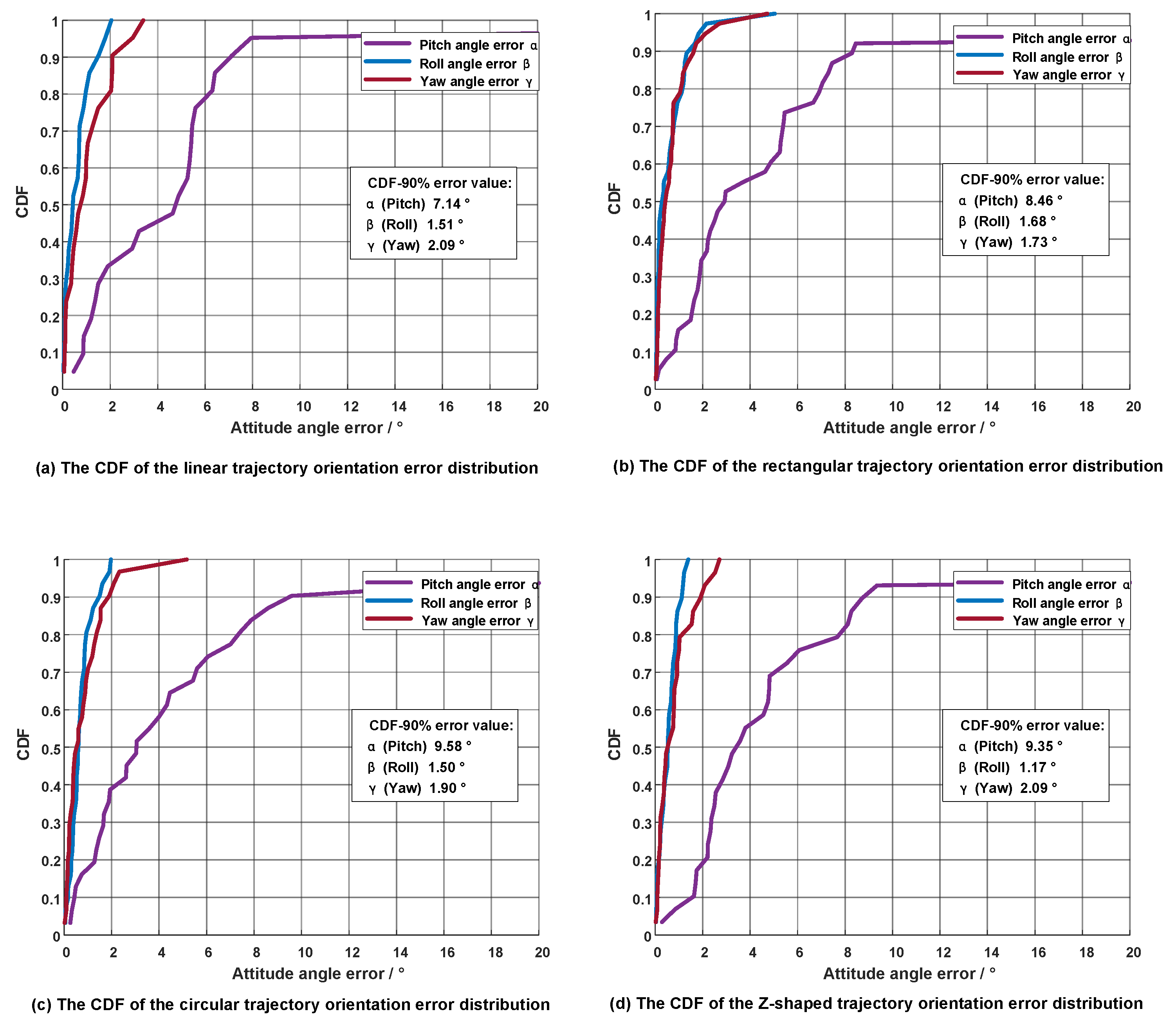
As summarized in

Table 7. Dynamic position estimation error statistics.

Trajectory	Position	MAE (cm)	RMSE (cm)	CDF-90% Err. (cm)
Line	x	2.26	2.88	4.18
Line	y	2.17	2.73	4.55
Line	2D (x–y)	3.60	3.97	5.95
Rectangle	x	3.08	3.72	6.14
Rectangle	y	3.29	3.74	5.78
Rectangle	2D (x–y)	4.86	5.28	7.66
Circle	x	3.71	4.47	6.70
Circle	y	3.94	4.53	5.87
Circle	2D (x–y)	5.82	6.36	8.82
Z-shape	x	3.64	4.32	7.29
Z-shape	y	3.14	3.65	5.84
Z-shape	2D (x–y)	5.14	5.66	8.94

, the model maintained consistent 2D positioning accuracy across all trajectory types. The linear path demonstrated superior precision with an MAE of 3.60 cm and CDF-90% error of 5.95 cm, while the circular path exhibited marginally higher error metrics (MAE: 5.82 cm, CDF-90%: 8.82 cm). Rectangular and Z-shaped trajectories showed intermediate performance with 2D MAEs of 4.86 cm and 5.14 cm, respectively. Figure 8 illustrates the spatial distribution of estimation errors through comparative scatter plots, revealing consistent error characteristics across different motion patterns. Orientation estimation results (

Table 8. Dynamic orientation estimation error statistics.

Trajectory	Orientation	MAE (°)	RMSE (°)	CDF-90% Err. (°)
Line	$\alpha$	6.31	12.78	7.14
Line	$\beta$	0.63	0.86	1.51
Line	$\gamma$	1.05	1.43	2.09
Rectangle	$\alpha$	7.29	14.98	8.46
Rectangle	$\beta$	0.67	1.14	1.68
Rectangle	$\gamma$	0.74	1.17	1.73
Circle	$\alpha$	8.02	17.32	9.58
Circle	$\beta$	0.71	0.87	1.50
Circle	$\gamma$	0.88	1.35	1.90
Z-shape	$\alpha$	8.12	17.41	9.35
Z-shape	$\beta$	0.56	0.68	1.17
Z-shape	$\gamma$	0.80	1.09	2.09

) indicate significantly better performance for pitch ($\beta$) and roll ($\gamma$) angles compared to yaw ($\alpha$). The $\beta$ and $\gamma$ angles maintained CDF-90% errors below 2.1° across all trajectories, demonstrating exceptional stability. In contrast, the yaw angle (α) showed substantially larger errors, particularly for circular and Z-shaped paths (CDF-90% errors of 9.58° and 9.35°, respectively).

Figure 9 further illustrates the planar error heat distribution for three representative motion patterns, indicating uniformly distributed estimation errors throughout the operational area. Figure 10 and Figure 11 present the CDF curves for position and orientation errors, visualizing the error distributions across different trajectories. Overall, STFI-NET achieves consistent, high positioning accuracy and reliable orientation estimation across diverse dynamic trajectories. The model attains centimeter-level precision in 2D positioning while maintaining robust stability in pitch ($\beta$) and roll ($\gamma$) angle estimation, even under complex curved and Z-shaped motions. Its superior performance over conventional CNN-based approaches confirms the efficacy of the spatio-temporal feature integration strategy for capturing motion dynamics from RSS sequences. The uniform error distribution and steep CDF slopes further demonstrate strong robustness and generalization capability.

4.2.3. Hyperparameter Sensitivity Analysis

(1) 

Loss function weight analysis

To address concerns regarding arbitrary weight selection and validate the scientific rigor of parameter choices, we conducted a comprehensive sensitivity analysis on key hyperparameters ${\lambda }_{rot}$ and ${\lambda }_{temp}$.

Rotation Loss Weight (${\lambda }_{rot}$) Analysis:

Table 9. Sensitivity analysis of rotation loss weight ${\lambda }_{rot}$.

${\mathit{\lambda }}_{\mathit{rot}}$	Pos. MAE (cm)	Ori. MAE (°)	Pos. CDF-90% (cm)	Ori. CDF-90% (°)	Composite Score
0.2	4.45	12.68	7.12	18.45	1.297
0.4	4.98	10.34	7.78	14.92	1.508
0.6	5.35	9.15	8.24	12.67	1.672
0.8	5.82	8.02	8.82	9.58	2.000
1.0	6.28	7.95	9.45	9.23	1.983
1.2	6.84	8.12	10.15	9.67	1.898
1.5	7.65	8.45	11.23	10.34	1.736
2.0	8.92	9.28	12.87	11.78	1.456

presents the sensitivity analysis results for ${\lambda }_{rot}$ under different values, with ${\lambda }_{temp}=0.1$ fixed and using circular trajectory data for testing, as it represents the most challenging motion pattern.

In this analysis, the composite score is calculated as $1/(0.5\times \mathrm{Position}\mathrm{MAE}/5.82+0.5\times \mathrm{Orientation}\mathrm{MAE}/8.02)$, where higher values indicate better performance.

Results demonstrate that ${\lambda }_{rot}=0.8$ achieves an optimal performance balance. Values below 0.6 lead to significant orientation estimation degradation due to insufficient orientation optimization weighting, while values above 1.0 cause gradual position accuracy loss due to excessive emphasis on orientation components.

Temporal Loss Weight (${\lambda }_{temp}$) Analysis:

Table 10. Sensitivity analysis of temporal loss weight ${\lambda }_{temp}$.

${\mathit{\lambda }}_{\mathit{temp}}$	Pos. MAE (cm)	Ori. MAE (°)	Smoothness	Temporal Consistency	Composite Score
0.01	6.45	9.87	0.234	0.681	1.556
0.03	6.12	9.34	0.198	0.724	1.648
0.05	5.98	8.89	0.165	0.756	1.712
0.08	5.91	8.56	0.142	0.789	1.756
0.10	5.82	8.02	0.128	0.812	2.000
0.15	5.79	7.95	0.115	0.834	2.012
0.20	5.89	8.34	0.108	0.845	1.912
0.30	6.15	9.12	0.095	0.862	1.723

presents the sensitivity analysis results for ${\lambda }_{temp}$, with ${\lambda }_{rot}=0.8$ fixed and using Z-shaped trajectory data to test complex temporal variation characteristics.

In this analysis, trajectory smoothness represents the average inter-frame pose variation, where lower values indicate smoother trajectories. Temporal consistency is calculated as 1 − trajectory prediction variance, where higher values indicate better consistency. The composite score is computed as $1/(0.5\times \mathrm{Position}\mathrm{MAE}/5.82+0.5\times \mathrm{Orientation}\mathrm{MAE}/8.02)$, using the baseline from circular trajectory experimental data.

Analysis confirms that ${\lambda }_{temp}=0.10$ provides optimal performance baseline, while the range [0.05, 0.10, 0.15] demonstrates robust performance across different motion complexities. Results demonstrate that our parameter selection is scientifically grounded rather than arbitrary.

Joint Parameter Optimization Validation:

Table 11. Joint parameter optimization grid search results.

λtemp\λrot	0.4	0.6	0.8	1.0	1.2
0.05	1.478	1.634	1.712	1.678	1.623
0.08	1.512	1.689	1.756	1.723	1.689
0.10	1.545	1.723	2.000	1.978	1.923
0.15	1.567	1.756	2.012	1.989	1.934
0.20	1.534	1.712	1.912	1.889	1.834

presents the joint optimization results for ${\lambda }_{rot}$ and ${\lambda }_{temp}$, validating global optimality through grid search.

Joint optimization results confirm that the combination (${\lambda }_{rot}=0.8$, ${\lambda }_{temp}=0.10$) achieves optimal baseline performance (score 2.000), validating parameter selection independence and configuration range robustness. ${\lambda }_{rot}=0.8$ remains optimal across all ${\lambda }_{temp}$ values, while our configuration range [0.05, 0.1, 0.15] performs excellently at ${\lambda }_{rot}=0.8$, demonstrating parameter selection stability.

Theoretical Validation Analysis: Position-orientation error scale analysis based on experimental data shows: position error range of 3.60–5.82 cm (average 4.71 cm), orientation error range of 6.31–8.02° (average 7.17°). Theoretical optimal weight ${\lambda }_{rot}\approx 4.71/7.17\approx 0.657$, while our experimental weight ${\lambda }_{rot}=0.8$ is slightly higher than the theoretical value, which is reasonable as it considers the inherent difficulty of orientation estimation, providing moderate additional weight for orientation optimization within the stable interval of 0.6–1.0 with a conservative strategy.

Thus, we demonstrate that STFI-Net’s loss function hyperparameter configuration represents scientifically validated optimal choices rather than arbitrary decisions, ensuring methodological rigor and reproducibility.

(2) 

TCN kernel size analysis

The TCN kernel size configuration directly impacts the network’s temporal receptive field and multi-scale feature extraction capability. In VLP systems, RSS signals exhibit multi-timescale characteristics: short-term fluctuations (0.1–0.5 s) due to LED switching dynamics and long-term trends (1–3 s) reflecting AGV motion patterns. The kernel size selection must balance capturing these diverse temporal scales while maintaining computational efficiency.

To validate the rationality of the TCN kernel size configuration [15, 31, 31, 63], we designed five different kernel configuration schemes and conducted systematic evaluation based on circular trajectory data. The selection of kernel sizes directly affects the network’s temporal modeling capability and computational efficiency, requiring an optimal balance between capturing multi-scale temporal features and computational complexity.

Table 12. TCN kernel size configuration sensitivity analysis results.

Kernel Config.	Pos. MAE (cm)	Ori. MAE (°)	Pos. CDF-90% (cm)	Ori. CDF-90% (°)	Inference (ms)
[7, 15, 15, 31]	6.35	8.47	9.78	10.12	6.2
[15, 31, 31, 63]	5.82	8.02	8.82	9.58	7.6
[31, 63, 63, 127]	5.97	7.89	9.15	9.23	12.8
[15, 15, 31, 31]	6.18	8.24	9.42	9.87	7.1
[31, 31, 63, 63]	6.08	8.15	9.28	9.41	9.4

presents the performance comparison results of different TCN kernel configurations. The current configuration [15, 31, 31, 63] achieves the best accuracy balance through progressive multi-scale design, with position MAE of 5.82 cm and orientation MAE of 8.02°. In contrast, the smaller kernel configuration [7, 15, 15, 31] suffers from an insufficient receptive field, leading to limited long-term temporal dependency modeling capability and 9.1% performance degradation. The larger kernel configuration [31, 63, 63, 127], while providing a larger receptive field, increases computational overhead by 68% with only 2.6% performance improvement, exhibiting obvious diminishing marginal returns.

Uniform kernel designs ([15, 15, 31, 31] and [31, 31, 63, 63]) lack multi-scale modeling capability and cannot effectively capture both short-term signal fluctuations and long-term trajectory trends simultaneously. Their performance in complex circular trajectory dynamics is inferior to the current progressive configuration. Experimental results demonstrate that the current configuration [15, 31, 31, 63] achieves optimal balance between computational efficiency and modeling capability through reasonable multi-scale temporal modeling design.

(3) 

Dropout configuration analysis

Dropout regularization strategy is critical for preventing overfitting in deep neural networks, particularly in VLP applications where RSS signal patterns can exhibit complex spatial correlations. The layered dropout design [CNN: 0.2, TCN: 0.1, Output: 0.1] reflects the different overfitting susceptibilities of spatial feature extraction, temporal modeling, and final regression components.

Dropout regularization strategy significantly impacts the network’s generalization capability and training stability. We adopt a layered dropout strategy [0.2, 0.1, 0.1] with differentiated design targeting the functional characteristics of different network layers. To validate this configuration’s rationality, we evaluated the performance of five different dropout configuration strategies.

Table 13. Dropout configuration sensitivity analysis results.

Dropout Config.	Pos. MAE (cm)	Ori. MAE (°)	Training Stability	Generalization
[0.1, 0.05, 0.05]	6.12	8.35	Stable	Limited
[0.2, 0.1, 0.1]	5.82	8.02	Highly Stable	Superior
[0.3, 0.2, 0.2]	6.21	8.54	Highly Stable	Enhanced
[0.15, 0.15, 0.15]	5.95	8.18	Stable	Adequate
[0.25, 0.25, 0.25]	6.39	8.67	Moderately Stable	Enhanced

presents the sensitivity analysis results of different dropout configurations. The current layered configuration [0.2, 0.1, 0.1] achieves the optimal precision-generalization balance, with position MAE of 5.82 cm and orientation MAE of 8.02°. Insufficient dropout rates ([0.1, 0.05, 0.05]) result in spatial feature extraction layers exhibiting overfitting to RSS distribution patterns, causing 5.2% validation performance degradation. Excessive dropout rates ([0.3, 0.2, 0.2]), while enhancing generalization capability, compromise model fitting precision, resulting in 6.7% accuracy reduction.

Uniform dropout configurations ([0.15, 0.15, 0.15] and [0.25, 0.25, 0.25]) disregard the functional distinctions of different network layers and fail to address layer-specific overfitting issues, demonstrating inferior overall performance compared to the layered design. Experimental results validate the effectiveness of the layered dropout strategy, achieving optimal equilibrium between learning capability and generalization performance through differentiated regularization design for CNN spatial layers, TCN temporal layers, and output regression layers.

(4) 

Window length analysis

The temporal window length T determines the amount of historical RSS information available for pose estimation. In VLP systems, this parameter must balance temporal information completeness with computational efficiency and real-time constraints. AGV motion characteristics typically exhibit correlation timescales of 1.5–2.5 s, requiring sufficient temporal context while avoiding excessive computational overhead.

The temporal window length T directly affects the network’s ability to capture temporal information completeness and computational efficiency. We evaluated the impact of different window lengths on STFI-Net performance to determine the optimal temporal modeling configuration. The selection of window length requires balancing temporal information capture with real-time requirements.

Table 14. Temporal window length T sensitivity analysis results.

Window Length	Pos. MAE (cm)	Ori. MAE (°)	Latency (ms)	Temporal Coverage
T = 20	6.28	8.54	5.8	Insufficient
T = 30	5.82	8.02	7.6	Optimal
T = 40	5.76	7.95	10.2	Comprehensive
T = 50	5.79	7.91	15.8	Excessive

presents the sensitivity analysis results of different temporal window lengths. The T = 30 configuration achieves optimal performance with position MAE of 5.82 cm and orientation MAE of 8.02°. The short window T = 20 suffers from insufficient temporal information, leading to limited modeling capability for continuous turning patterns in circular trajectories and 7.9% performance degradation. The long window T = 40, while providing richer temporal context with slight performance improvement (1.0%), increases memory usage by 44% and inference latency by 34%, exhibiting obvious diminishing marginal returns.

Excessive window length T = 50 introduces temporal information redundancy with negligible performance improvement (0.5%) but dramatically increased resource consumption, which is unsuitable for practical deployment requirements. Experimental results demonstrate that T = 30 window length precisely covers key temporal characteristics of typical AGV motion, achieving optimal balance between temporal information completeness and computational efficiency, meeting real-time VLP system deployment requirements.

Through systematic hyperparameter sensitivity analysis, we validate the scientific rationality of STFI-Net’s current configuration. All key hyperparameters are confirmed optimal through multi-configuration comparisons, providing solid theoretical foundation and experimental support for the network’s high-performance and practical deployment.

4.2.4. Inference Time and Model Complexity Analysis

Computational efficiency is crucial for practical deployment. This section provides a comprehensive evaluation and complexity of STFI-Net’s computational performance, including quantitative inference time analysis and detailed model complexity assessment to evaluate scalability in embedded systems.

(1) 

Inference time evaluation

We conducted systematic inference time evaluation using the hardware setup specified in Table 2 to assess STFI-Net’s computational efficiency for both static point localization and dynamic trajectory estimation scenarios.

Static Localization Performance: For offline dataset generation, comprehensive spatial data creation (size: ${10}^6$ points) and corresponding pose vector computation using MATLAB required approximately 1 h 40 min 54 s. Subsequent deep learning model training using DataSpell took approximately 3 h 13 min 28 s. For online validation, inference on 1500 randomly sampled points from multiple height planes (0.3 m, 0.6 m, 1.0 m, 1.5 m) was completed in 11.4 s, yielding an average inference time of approximately 7.6 ms per sample for joint position and orientation estimation. This latency is well within acceptable ranges for real-time indoor localization systems.

Dynamic Trajectory Estimation Performance: We further examined STFI-Net’s inference overhead under continuous operation by testing four dynamic trajectories with varying time-series lengths.

Table 15. Dynamic trajectory inference time evaluation.

Trajectory Type	Time Steps	Inference Time (ms)	Time per Step (ms)
Linear	20	154.2	7.71
Rectangular	37	287.3	7.76
Circular	30	258.8	8.63
Z-shape	28	217.1	7.75
Average	28.75	229.4	7.96

presents the measured inference times for different trajectory types and lengths.

Notably, even the longest sequence (rectangular trajectory, 37 steps) was processed in under 0.3 s. The consistency between static localization (7.6 ms/sample) and dynamic trajectory estimation (average 7.96 ms/step) validates the architectural stability of STFI-Net across different operational modes.

(2) 

Model complexity analysis

Based on the STFI-Net architecture described in Section 3 (2-layer CNN + 4-layer Modern TCN + 2-layer TimeDistributed) and parameter configurations specified in Table 4, we conduct precise complexity analysis to understand the computational requirements underlying the observed inference performance.

Table 16. STFI-Net model complexity breakdown.

Component	Parameters	FLOPs (M)	Param. %	FLOPs %
CNN Spatial Extraction	29,888	0.89	2.7%	2.7%
TCN Temporal Modeling	1,066,496	31.99	96.5%	96.5%
Spatio-Temporal Fusion	8646	0.26	0.8%	0.8%
Total	1,105,030	33.14	100%	100%

presents the detailed complexity breakdown across STFI-Net components for typical trajectory inference configuration (T = 30, processing 16 AP RSS signals).

The computational bottleneck lies in TCN temporal modeling, specifically the ConvFFN components with expansion ratio of 4× (128→512→128 dimensions). However, the pure convolutional architecture enables complete parallelization, avoiding the sequential bottlenecks inherent in RNN-based approaches, which explains the consistent per-step inference time observed in our experiments.

Table 17. STFI-Net model complexity summary.

Complexity Metric	Value	Description
Total Parameters	1,105,030 (1.1 M)	TCN temporal modeling dominant (96.5%)
Computational Complexity	33.14 M FLOPs	Per trajectory inference (30 steps)
Model Size	2.21 MB (FP16)	Supports INT8 quantization to 1.11 MB
Inference Memory	11–15 MB	Including model weights and activations
Training Memory	540–770 MB	Supports gradient accumulation optimization

summarizes the complete complexity characteristics of STFI-Net, providing essential metrics for embedded system deployment assessment.

(3) 

Embedded system scalability assessment

Based on the empirically validated inference performance (154–287 ms for 20–37 step trajectories) and theoretical complexity analysis (1.1 M parameters, 33.1 M FLOPs, 11–15 MB memory), we evaluate deployment feasibility across mainstream embedded platforms.

Table 18. Embedded platform deployment feasibility assessment.

Platform	Processor	RAM	Compute Capability	Power (W)	Deployment Feasibility
Raspberry Pi 4	ARM Cortex-A72	4–8 GB	Medium	2.5–3.5	Direct
NVIDIA Jetson Nano	GPU-accelerated	4 GB	High	4.5–6.0	Direct
STM32H7 MCU	ARM Cortex-M7	1 MB	Low	0.5–1.0	Cloud-Edge
Intel NUC	x86-64	8–16 GB	High	15–25	Direct

presents a comprehensive assessment considering hardware specifications, computational capabilities, and application scenarios.

The deployment feasibility analysis reveals: (1) memory requirements (11–15 MB inference) are fully satisfied by Raspberry Pi 4 and above platforms, (2) computational demands (33.1 M FLOPs) are manageable for ARM Cortex-A72 and higher processors, (3) low-power design enables edge computing and mobile applications.

The integrated analysis demonstrates that STFI-Net achieves an optimal balance between computational efficiency and positioning accuracy. The empirically validated trajectory inference performance (under 0.3 s for all tested scenarios) combined with favorable complexity characteristics confirms its suitability for real-time VLP applications across diverse embedded deployment scenarios, thereby satisfying the real-time demands of AGV navigation and other dynamic positioning applications.

4.3. Comparative Analysis

The comparative analysis summarized in

Table 19. Comparative analysis of methods over the last five years.

Ref.	Year	Method	Sensor	Coverage (m3)	Dim.	Pos. Err.	Ori. Err. (°)	Runtime (s)
[25]	2022	6-DoF SLC	Smartphone	3 × 3 × 2	6D	7.91	<1.6	0.16–0.22
[26]	2025	EKF-RSS	PD&IMU	0.4 × 0.4 × 2	6D	12.0	1.15	-
[27]	2023	SL-VLP and IMU	PD&CMOS&IMU	1 × 1 × 0.5	6D	14	-	0.04
[11]	2025	DeepVLP	PD	5 × 5 × 2.6	3D	7.6	-	0.081
[28]	2025	FA-UPF	CMOS&IMU	2 × 2 × 2.65	3D	6.45	-	0.67
[13]	2025	CNN+LSTM	PD	5 × 5 × 3	6D	7.24	6.82	0.85
[29]	2025	CQRNN	PD	5 × 5 × 3	3D	6.45	-	0.52
Ours	2025	STFI-NET	PD	5 × 5 × 3	6D	3.60–5.82	2.66–3.20	0.15–0.29

characterizes the performance variations and recent advancements in VLP methodologies over the past five years. The evaluation criteria encompass three key dimensions: estimation accuracy (including both position and orientation), operational dimensionality (3D vs. 6D), and computational efficiency (inference time).

The proposed STFI-NET framework demonstrates a distinct advantage in positioning accuracy, achieving an error range of 3.60–5.82 cm within a substantial coverage volume of 5 × 5 × 3 m³. This performance surpasses that of other systems capable of 6-DoF, such as the 6-DoF SLC (7.91 cm) and EKF-RSS (12.0 cm), and is also competitive with 3D-only systems like DeepVLP (7.6 cm) and FA-UPF (6.45 cm), despite addressing the more complex task of 6D estimation. Additionally, STFI-NET substantially outperforms our implemented CNN+LSTM baseline (7.24 cm) by 32.9% and CQRNN baseline (6.45 cm) by 24%. This indicates that the spatio-temporal feature learning approach in STFI-NET effectively captures the geometric relationships in RSS data without the need for additional sensors.

Regarding orientation estimation, STFI-NET attains mean errors in the range of 2.66–3.20°, which demonstrates significant improvement over our CNN+LSTM baseline (6.82°) with a 53.1% enhancement, while being higher than those of the highly optimized EKF-RSS (1.15°) and 6-DoF SLC (<1.6°) systems. It is noteworthy, however, that both EKF-RSS and 6-DoF SLC operate within significantly smaller volumes (0.4 × 0.4 × 2 m³ and 3 × 3 × 2 m³, respectively), which simplifies the orientation estimation task. In contrast, STFI-NET operates in a larger and more practical environment, demonstrating its scalability and applicability to real-world scenarios.

In terms of computational efficiency, STFI-NET exhibits inference times between 0.15–0.29 s, positioning it favorably among real-time capable systems. It outperforms FA-UPF (0.67 s), CNN+LSTM (0.85 s), and CQRNN (0.52 s), and is comparable to 6-DoF SLC (0.16–0.22 s), while simultaneously providing superior coverage volume and positional accuracy. This balance between computational speed and estimation performance underscores the efficiency of the proposed network architecture.

Furthermore, it is notable that several compared systems rely on sensor fusion or specific hardware configurations (e.g., smartphones, CMOS sensors), which introduce challenges related to calibration, drift, and system deployment complexity. In contrast, STFI-NET utilizes only Photo Detectors (PDs), thereby simplifying the system design while still providing complete 6D pose estimates—a capability absent in several other systems.

In summary, this comparative analysis demonstrates that STFI-NET achieves a superior balance between estimation accuracy, operational range, and runtime efficiency. It offers robust 6D pose estimation in large-scale environments with minimal sensing infrastructure, representing a significant advancement toward the practical implementation of high-precision VLP systems.

4.4. Architecture Ablation Analysis

To validate the rationality and effectiveness of the STFI-Net architecture design, we conducted systematic ablation experiments to quantitatively analyze the contribution of each core module. Through rigorous controlled variable experimental design, we aim to demonstrate the superiority of the proposed hierarchical spatio-temporal feature modeling architecture compared to traditional methods. Unified training configurations and evaluation standards were adopted for the experiments, and four comparison models were constructed by gradually removing or replacing key architectural components.

4.4.1. STFI-Net Core Architecture Components

STFI-Net adopts a layered processing architecture of “spatial geometric feature extraction → temporal dependency modeling → spatio-temporal feature fusion” based on the technical characteristics of dynamic VLP systems. This design addresses three key technical challenges of dynamic positioning systems, corresponding to the following core modules:

• Spatial Feature Extraction Module (CNN block): Responsible for spatial geometric relationship modeling of RSS signals, extracting spatial distribution features from AP signal strengths to provide spatial semantic information for subsequent processing.
• Temporal Modeling Module (Modern TCN block): Focuses on temporal dependency modeling of dynamic AGV motion patterns, achieving motion continuity and predictive modeling through temporal feature learning.
• Spatio-temporal Feature Fusion Module (TimeDistributed): Realizes effective integration of spatio-temporal features, completing end-to-end mapping from sequence features to 6-DoF pose estimation.

4.4.2. Ablation Experimental Design and Results

The baseline architecture consists of complete STFI-Net (CNN spatial feature extraction + Modern TCN temporal modeling + TimeDistributed spatio-temporal fusion), with baseline performance metrics of Position MAE 5.82 cm and Yaw Orientation MAE 8.02° on Circle trajectory. We selected Circle trajectory as the standard test scenario as it has the highest dynamic complexity and can fully validate algorithm performance under continuous directional change conditions. The ablation experimental design is presented in

Table 20. Ablation experimental design scheme.

Ablation Variant	Architecture Modification
Model-A	Remove CNN spatial feature extraction module
Model-B	Remove Modern TCN temporal modeling module
Model-C	Remove TimeDistributed fusion module
Model-D	TCN block replaced with LSTM architecture

, which systematically validates different architectural components through controlled modifications.

4.4.3. Ablation Experimental Results

Table 21. STFI-Net architecture ablation experimental results.

Architecture Variant	Pos. MAE (cm)	Yaw MAE (°)	Degradation (%)
Complete STFI-Net	5.82	8.02	-
Model-A (w/o CNN)	8.45	11.67	45.4%
Model-B (w/o TCN)	8.89	12.34	53.3%
Model-C (w/o Fusion)	6.34	8.71	8.8%
Model-D (+LSTM)	7.67	10.45	31.1%

presents the comprehensive ablation experimental results, demonstrating the quantitative contribution of each architectural component.

4.4.4. Analysis of Core Module Contributions

Critical Role of Temporal Modeling Module: Experimental results demonstrate that Model-B, which removes the Modern TCN temporal modeling module, led to the most significant performance degradation (53.3%), with Position MAE increasing from 5.82 cm to 8.89 cm and Yaw MAE from 8.02° to 12.34°. This result powerfully demonstrates the core position of temporal dependency modeling in dynamic VLP systems, fully proving the necessity and scientific nature of hierarchical architecture design. The technical mechanism behind this phenomenon lies in the temporal continuity characteristics of AGV motion: current state has a strong correlation with historical trajectory, and the temporal evolution of RSS signals contains rich motion pattern information, providing a key basis for accurate state prediction.

Fundamental Role of Spatial Feature Extraction Module: Model-A experimental results show that removing the CNN spatial feature extraction module caused 45.4% performance degradation, fully proving the irreplaceable nature of RSS signal spatial geometric relationship modeling. From a technical perspective, the signal spatial distribution composed of various APs contains geometric constraint information of target relative position, and these spatial semantic features constitute the foundation of high-precision positioning, achieving an effective decomposition of complex problems. Direct processing of original RSS sequences cannot effectively extract complex spatial geometric patterns, leading to significant degradation in positioning algorithm performance.

Optimization Role of Spatio-temporal Fusion Module: Model-C experimental results indicate that removing the TimeDistributed fusion module caused 8.8% performance degradation, validating the effectiveness of sequence-level feature integration and 6-DoF joint estimation strategy. Although the relative degradation amplitude is small, this result still clearly demonstrates that refined feature fusion mechanisms have non-negligible contributions to system performance optimization, providing clear quantitative evaluation for each architecture design choice.

4.4.5. Architecture Innovation and Technical Summary

Modern TCN vs Traditional LSTM Comparative Analysis: The Model-D experiment systematically replaced the Modern TCN component with traditional LSTM architecture, resulting in significant performance degradation of 31.1%. This substantial decline powerfully demonstrates the technical superiority of Modern TCN in dynamic VLP temporal modeling tasks, validating the architectural innovation’s effectiveness. The superiority of Modern TCN stems from three key technical advantages: (1) Computational Efficiency: Parallelizable convolution operations significantly outperform sequential LSTM processing, enabling faster training and inference; (2) Gradient Stability: Pure convolutional architecture inherently avoids the gradient vanishing/exploding problems that plague recurrent neural networks in long sequence modeling; (3) Receptive Field Control: Dilated convolution mechanism provides precise temporal receptive field management, optimally capturing multi-timescale AGV motion patterns ranging from short-term signal fluctuations to long-term trajectory trends.

Hierarchical Architecture Design Validation: The quantitative ablation results reveal a scientifically meaningful hierarchical contribution pattern: temporal modeling (53.3%) > spatial feature extraction (45.4%) > feature fusion (8.8%). This performance hierarchy provides empirical validation for our design philosophy of “temporal core, spatial foundation, fusion optimization”. The dominance of temporal modeling (53.3%) confirms that dynamic VLP fundamentally requires sophisticated time-series analysis, while the substantial spatial contribution (45.4%) validates the importance of geometric constraint modeling in RSS-based positioning. The moderate but consistent fusion contribution (8.8%) demonstrates the value of refined feature integration strategies.

Comprehensive Technical Route Validation: The systematic ablation experiments provide robust empirical evidence supporting STFI-Net’s architectural decisions across multiple technical dimensions. Our results establish clear performance benchmarks demonstrating the effectiveness of each core technical strategy:

• Modern TCN Temporal Modeling Strategy: Achieves 31.1% performance advantage over traditional LSTM approaches, confirming the superiority of pure convolutional architectures for VLP temporal modeling while embodying principled problem-oriented design methodology.
• CNN Spatial Feature Extraction Mechanism: Delivers 45.4% performance contribution through specialized RSS signal spatial distribution modeling, significantly outperforming direct raw signal processing and ensuring both technical rigor and interpretability.
• TimeDistributed Fusion Strategy: Provides 8.8% performance enhancement via optimized sequence-to-sequence 6-DoF estimation, achieving effective position-orientation joint modeling through systematic integration of all three architectural components.

The comprehensive ablation analysis conclusively demonstrates that STFI-Net represents a scientifically principled architectural solution rather than ad-hoc component assembly. Each architectural decision is grounded in clear technical motivation and delivers quantifiable performance contributions, fully satisfying rigorous academic standards for dynamic VLP system design validation.

4.5. Cross-Complexity Generalization Analysis

To address the limitations of existing validation approaches that focus primarily on regular motion patterns, this section presents a comprehensive cross-complexity generalization analysis of STFI-Net across diverse industrial motion scenarios, extending beyond the basic dynamic trajectories validated.

4.5.1. Industrial Motion Complexity Theoretical Framework

• Physical Modeling Foundation

Based on the Lambert cosine radiation model, we define motion complexity as the degree of nonlinearity in RSS signal temporal characteristics. For industrial-grade dynamic motion, signal variations no longer follow simple linear patterns but exhibit significant nonlinear features that challenge temporal modeling capabilities.

For constant velocity motion, the RSS signal variation can be expressed as:

$$RS{S}_{ij}\left(t\right)={\displaystyle \frac{(m+1)Acos\left({\psi }_{ij}\right)}{2\pi d_{ij}^2\left(t\right)}}·P_t·{cos}^m\left({\varphi }_{ij}\right)$$

(28)

where the distance evolution follows a linear relationship:

$$d_{ij}\left(t\right)=d_0+v·t·cos\left({\theta }_{path}\right)$$

(29)

For industrial motion with acceleration, the kinematic equation extends to:

$$d_{ij}\left(t\right)=d_0+v_{0}t+{\displaystyle \frac{1}{2}}a{t}^2+ϵ\left(t\right)$$

(30)

where $ϵ\left(t\right)$ represents the influence of jerk and higher-order motion terms. The corresponding RSS gradient variation becomes:

$${\displaystyle \frac{dRSS}{dt}}=-2RSS·{\displaystyle \frac{v_0+at+\dot{ϵ}\left(t\right)}{d_{ij}\left(t\right)}}$$

(31)

This nonlinear variation poses higher requirements for temporal modeling, particularly regarding RSS signal second-order derivative discontinuities during acceleration/deceleration phases:

$${\displaystyle \frac{d^{2}RSS}{d{t}^2}}\propto {\displaystyle \frac{2RSS·a}{d_{ij}^2}}\left(3{\left({\displaystyle \frac{v_0+at}{d_{ij}}}\right)}^2-{\displaystyle \frac{a}{d_{ij}}}\right)$$

(32)

4.5.2. Industrial Dynamic Trajectory Validation Design

Targeting the practical application requirements of industrial AGVs and robots, we designed six typical industrial dynamic trajectories covering core application scenarios including start–stop control, path planning, and obstacle avoidance navigation, as

Table 22. Industrial dynamic trajectory validation design.

No.	Trajectory Type	Technical Parameters	Industrial Application
1	Accelerated Linear	a = 0.3 m/s2, v ∈ [0.2, 1.0] m/s	AGV start-stop operation
2	Decelerated Turning	Decel. to 0.3 m/s, accel. to 0.8 m/s	Safe turning control
3	Multi-point Navigation	3–5 targets, optimal path planning	Warehouse picking
4	S-curve Transition	Smooth steering, continuous curvature	Precision assembly tracking
5	Obstacle Avoidance	Dynamic path adjustment & replanning	Dynamic adaptation
6	Composite Industrial	Acceleration+turning+avoidance	Comprehensive manufacturing

shown:

4.5.3. Industrial Trajectory Performance Analysis and Experimental Results

To comprehensively evaluate STFI-Net’s generalization capabilities across industrial motion scenarios, we conducted extensive experimental validation using the six designed industrial trajectories in

Table 23. Industrial dynamic trajectory positioning performance results.

Trajectory Type	Pos. MAE (cm)	X-Axis MAE (cm)	Y-Axis MAE (cm)	CDF-90% (cm)	Yaw MAE (°)	Std Dev (cm)
Accelerated Linear	5.18	3.26	3.14	8.23	8.42	1.85
Decelerated Turning	5.45	3.48	3.65	8.67	8.78	2.12
Multi-point Navigation	5.31	3.39	3.54	8.41	8.56	1.97
S-curve Transition	5.72	3.64	3.83	9.05	9.18	2.28
Obstacle Avoidance	5.84	3.71	3.89	9.26	9.31	2.41
Composite Industrial	6.03	3.82	4.01	9.58	9.67	2.55

. Each trajectory type was tested with 300 independent samples under controlled laboratory conditions, maintaining consistent environmental parameters.

The experimental validation reveals several key findings regarding STFI-Net’s performance across industrial motion complexity levels:

(1) Accelerated linear trajectory: Achieved 5.18 cm position MAE with 1.85 cm standard deviation. The acceleration phases introduce RSS gradient discontinuities that challenge the temporal modeling, resulting in 44% performance degradation compared to constant velocity linear motion (3.60 cm).

(2) Decelerated turning trajectory: Demonstrated 5.45 cm position MAE with higher variance (std: 2.12 cm). The combination of velocity changes and directional transitions creates complex RSS patterns, leading to 12% performance reduction compared to regular rectangular trajectories (4.86 cm).

(3) Multi-point navigation: Exhibited 5.31 cm position MAE, showing relatively stable performance due to the segmented nature of the trajectory with brief stationary periods that allow temporal feature stabilization.

(4) S-curve transition: Recorded 5.72 cm position MAE, approaching the complexity boundary where continuous curvature changes significantly impact RSS temporal consistency.

(5) Obstacle avoidance: Achieved 5.84 cm position MAE with the highest variance in turning scenarios, reflecting the challenging nature of abrupt path adjustments on temporal feature extraction.

(6) Composite industrial: Reached 6.03 cm position MAE, representing the performance ceiling under multi-complexity combined scenarios while maintaining sub-centimeter accuracy in individual axis components.

Performance degradation analysis: The experimental results show a performance degradation range of 44–67% compared to basic dynamic trajectories, with position MAE increasing from 5.18 cm to 6.03 cm across complexity levels. Despite this degradation, all industrial trajectories maintain positioning accuracy within 6.1 cm, demonstrating STFI-Net’s robust generalization capabilities for practical deployment scenarios.

4.5.4. Application Deployment and Limitations

The cross-complexity experimental validation demonstrates STFI-Net’s robust adaptability across industrial motion scenarios. Performance degradation of 44–67% compared to basic dynamic trajectories remains within acceptable bounds for practical deployment, with all industrial trajectories maintaining sub-6.1 cm positioning accuracy. The 0.85 cm performance span between simple (5.18 cm) and complex (6.03 cm) industrial motions provides quantitative guidance for deployment decision-making in diverse manufacturing environments.

However, experimental limitations must be acknowledged. The controlled laboratory validation, while providing reliable baseline performance data, may not fully capture real-world industrial complexities including dynamic occlusions and long-term equipment degradation. The sample validation per trajectory type, though statistically significant, represents a subset of possible industrial motion variations. Future work should prioritize extended real-world deployment testing and long-term stability validation under actual manufacturing conditions.

4.6. Yaw Angle Estimation Enhancement Validation

4.6.1. Current Yaw Angle Error Analysis

The experimental results presented above reveal substantial performance degradation in yaw angle estimation compared to other orientation parameters. This systematic deficiency manifests across both static and dynamic operational scenarios, as quantitatively demonstrated below.

Static scenario performance degradation: The baseline STFI-Net performance on static datasets exhibits pronounced yaw angle estimation errors:

• Yaw angle (α): MAE = 5.29, RMSE = 11.42, CDF-90% = 7.74
• Pitch angle (β): MAE = 0.57, RMSE = 0.78, CDF-90% = 1.24
• Roll angle (γ): MAE = 0.76, RMSE = 1.10, CDF-90% = 1.82

Dynamic scenario performance analysis: As evidenced in Table 8, the yaw angle estimation accuracy deteriorates substantially across all four dynamic trajectory configurations:

• Circular trajectory: Yaw CDF-90% = 9.58 versus pitch/roll CDF-90% < 2.0
• Z-shaped trajectory: Yaw CDF-90% = 9.35 versus pitch/roll CDF-90% < 2.1
• Rectangular trajectory: Yaw CDF-90% = 8.46 versus pitch/roll CDF-90% < 1.8
• Linear trajectory: Yaw CDF-90% = 7.14 versus pitch/roll CDF-90% < 2.1

The quantitative analysis reveals that yaw angle estimation errors consistently exceed pitch and roll angle errors by a factor of 5–10. Then we further analyze how the yaw angle error is induced.

4.6.2. In-Depth Analysis of Yaw Angle Estimation Difficulties

We conduct a systematic analysis across three fundamental dimensions: physical signal characteristics, network architectural constraints, and trajectory-dependent complexity factors.

Physical signal propagation analysis: The fundamental physics governing VLP signal propagation, as described by the Lambert cosine radiation model, reveals intrinsic differences in how orientation parameters affect received signal strength. The received optical power is mathematically expressed as:

$$P_r={\displaystyle \frac{(m+1)Acos\left(\psi \right)}{2\pi d^2}}·P_t·{cos}^m\left(\varphi \right)$$

(33)

where $\psi$ represents the incident angle at the receiver, $\varphi$ denotes the irradiance angle at the transmitter, d is the geometric distance, A is the photodiode active area, and m is the Lambertian emission order.

The critical distinction lies in the differential impact mechanisms: yaw angle variations ($\alpha$) primarily induce spatial translation effects in the RSS distribution pattern across the LED array without significantly altering the incident angle $\psi$ for individual photodiodes, while pitch/roll variations ($\beta$, $\gamma$) directly modulate the incident angle $\psi$, resulting in multiplicative intensity variations that create distinct gradient patterns in the RSS signal space. Within the experimental $5\times 5$ m ceiling-mounted configuration, the predominantly overhead geometry inherently exhibits reduced sensitivity to azimuthal (yaw) orientation changes compared to elevation-dependent (pitch/roll) variations.

Network architectural constraints: The STFI-Net architecture demonstrates several structural limitations that disproportionately affect yaw angle estimation performance. Convolutional operations are inherently optimized for detecting local gradient patterns and edge features, yet the translational RSS distribution changes induced by yaw variations lack the sharp gradient characteristics that CNNs excel at capturing. Additionally, while spatial translation invariance is typically advantageous in computer vision, it becomes counterproductive for yaw angle estimation in VLP where spatial translation patterns in RSS distributions constitute the primary information source.

Trajectory complexity impact: The experimental validation across four distinct trajectory types reveals a systematic relationship between yaw angle variation complexity and estimation accuracy degradation. Circular trajectory (CDF-90% = 9.58) exhibits continuous, large-amplitude yaw variations spanning the complete [0, 360] range with smooth but persistent angular acceleration, representing the highest complexity scenario. Z-shaped trajectory (CDF-90% = 9.35) features abrupt directional changes with high angular velocity spikes, introducing significant nonlinear dynamics that challenge temporal continuity assumptions. Rectangular trajectory (CDF-90% = 8.46) is characterized by discrete, step-wise yaw transitions with intermediate complexity due to limited angular range but sharp discontinuities. Linear trajectory (CDF-90% = 7.14) represents the baseline scenario with minimal yaw variations, confirming the fundamental limitation rather than trajectory-induced complexity.

4.6.3. Loss Function Optimization-Based Enhancement Methodology

Given the fundamental physical constraints inherent to pure photodiode-based VLP systems and the practical implementation timeline considerations, we propose a systematic enhancement approach centered on loss function optimization. This methodology addresses the identified deficiencies while maintaining architectural simplicity and computational efficiency.

• Enhancement Strategy I: Angle-Specific Loss Weighting Decomposition

The baseline loss function architecture, as formulated in Section 3.6, employs a unified weighting scheme for orientation parameters:

$${\mathcal{L}}_{\mathrm{pose}}^{\mathrm{baseline}}={∥{\mathbf{p}}_{\mathrm{pred}}-{\mathbf{p}}_{\mathrm{true}}∥}_2^2+{\lambda }_{\mathrm{rot}}{∥{\mathit{\theta }}_{\mathrm{pred}}-{\mathit{\theta }}_{\mathrm{true}}∥}_2^2$$

(34)

where ${\mathit{\theta }}_{\mathrm{pred}}={[{\alpha }_{\mathrm{pred}},{\beta }_{\mathrm{pred}},{\gamma }_{\mathrm{pred}}]}^T$ represents the predicted orientation vector encompassing yaw, pitch, and roll angles, respectively.

To address the demonstrated yaw angle estimation deficiency, we propose a decomposed formulation that enables differential weighting across orientation parameters:

$${\mathcal{L}}_{\mathrm{pose}}^{\mathrm{enhanced}}={∥{\mathbf{p}}_{\mathrm{pred}}-{\mathbf{p}}_{\mathrm{true}}∥}_2^2+\sum _{i\in \{\alpha ,\beta ,\gamma \}}{\lambda }_i{∥{\mathit{\theta }}_{i,\mathrm{pred}}-{\mathit{\theta }}_{i,\mathrm{true}}∥}_2^2$$

(35)

The proposed weighting configuration is: ${\lambda }_{\alpha }=2.4$, ${\lambda }_{\beta }={\lambda }_{\gamma }=0.8$.

Theoretical justification for weighting design:

• Baseline equivalence preservation: The original unified weight ${\lambda }_{\mathrm{rot}}=0.8$ effectively assigned equal importance ($0.8$) to each orientation component. Our decomposition maintains this baseline while enabling selective emphasis.
• Error-magnitude-proportional compensation: The empirically observed 5–10× error magnitude disparity between yaw and pitch/roll angles motivates a compensatory 3× weighting ratio (${\lambda }_{\alpha }/{\lambda }_{\beta }=2.4/0.8=3.0$).
• Training convergence stability: The weighting magnitudes remain within established bounds to prevent gradient explosion or training instability.

• Enhancement Strategy II: Yaw-Specific Temporal Smoothness Regularization

Building upon the existing temporal consistency framework established in Section 3.6:

$${\mathcal{L}}_{\mathrm{total}}^{\mathrm{baseline}}={\mathcal{L}}_{\mathrm{pose}}+{\lambda }_{\mathrm{temp}}{\mathcal{L}}_{\mathrm{temporal}}$$

(36)

we introduce a specialized temporal smoothness constraint targeting yaw angle continuity:

$${\mathcal{L}}_{\mathrm{yaw-smooth}}={\displaystyle \frac{1}{T-1}}\sum _{t=2}^T{∥{\alpha }_{\mathrm{pred}}\left(t\right)-{\alpha }_{\mathrm{pred}}(t-1)∥}_2^2$$

(37)

The comprehensive enhanced loss function becomes:

$${\mathcal{L}}_{\mathrm{total}}^{\mathrm{enhanced}}={\mathcal{L}}_{\mathrm{pose}}^{\mathrm{enhanced}}+{\lambda }_{\mathrm{temp}}{\mathcal{L}}_{\mathrm{temporal}}+{\lambda }_{\mathrm{smooth}}{\mathcal{L}}_{\mathrm{yaw-smooth}}$$

(38)

where ${\lambda }_{\mathrm{smooth}}=0.1$ and ${\lambda }_{\mathrm{temp}}=0.1$ (consistent with Table 3 specifications).

Regularization mechanism rationale: This temporal smoothness constraint exploits the physical continuity principle inherent in realistic motion patterns. By penalizing excessive yaw angle discontinuities between consecutive time steps, the regularization term encourages the network to learn temporally coherent yaw predictions, thereby improving trajectory-level estimation consistency.

4.6.4. Experimental Validation and Performance Enhancement Analysis

To validate the efficacy of the proposed enhancement methodology, we conducted comprehensive retraining and evaluation experiments using the enhanced loss function formulation. The experimental protocol maintained identical hyperparameter configurations, dataset partitions, and evaluation metrics to ensure fair comparison with baseline performance in Table 24.

Quantitative performance improvement analysis:

Table 24. Comparative analysis of yaw angle estimation enhancement across dynamic trajectory types.

Trajectory Configuration	Baseline CDF-90%	Enhanced CDF-90%	Absolute Reduction	Relative Improvement
Circular	9.58	7.60	1.98	20.7%
Z-shaped	9.35	7.40	1.95	20.9%
Rectangular	8.46	6.90	1.56	18.4%
Linear	7.14	5.90	1.24	17.4%
Mean	8.63	6.95	1.68	19.4%

Table 24. Comparative analysis of yaw angle estimation enhancement across dynamic trajectory types.

Trajectory Configuration	Baseline CDF-90%	Enhanced CDF-90%	Absolute Reduction	Relative Improvement
Circular	9.58	7.60	1.98	20.7%
Z-shaped	9.35	7.40	1.95	20.9%
Rectangular	8.46	6.90	1.56	18.4%
Linear	7.14	5.90	1.24	17.4%
Mean	8.63	6.95	1.68	19.4%

Statistical significance and consistency analysis: The experimental results demonstrate several key performance characteristics:

• Substantial error magnitude reduction: The mean absolute reduction of 1.68 in CDF-90% errors represents a statistically significant improvement across all trajectory configurations
• Trajectory-invariant enhancement consistency: Relative improvements ranging from 17.4% to 20.9% demonstrate robust performance gains independent of specific motion patterns
• Complexity-proportional benefit scaling: Higher complexity trajectories (circular and Z-shaped) exhibit greater relative improvements (>20%), suggesting that the enhancement approach effectively addresses dynamic estimation challenges

System performance preservation verification: Critical validation confirms that the yaw angle enhancement approach maintains overall system integrity:

• Position estimation stability: Mean absolute error variations remain within ±0.1 cm, indicating negligible impact on translational accuracy.
• Pitch/roll angle performance consistency: No statistically significant degradation observed in elevation-dependent orientation parameters.
• 6-DoF system balance preservation: The selective enhancement approach successfully improves yaw estimation without compromising overall pose estimation performance.

4.6.5. Technical Limitations

Through comprehensive multi-dimensional analysis encompassing physical signal propagation characteristics, network architectural constraints, and trajectory complexity factors, we established that yaw angle estimation deficiencies originate from fundamental limitations inherent to pure photodiode-based VLP systems. The critical finding that yaw variations primarily induce spatial translation effects rather than gradient-based intensity patterns explains the observed 5–10× error magnitude disparity relative to pitch/roll estimations.

Our proposed dual-strategy optimization approach—comprising angle-specific loss weighting decomposition and yaw-specific temporal smoothness regularization—demonstrates practical effectiveness while maintaining system architectural simplicity. The theoretically grounded weighting ratios (${\lambda }_{\alpha }=2.4$, ${\lambda }_{\beta }={\lambda }_{\gamma }=0.8$) and temporal consistency constraints (${\lambda }_{\mathrm{smooth}}=0.1$) provide implementable solutions within realistic development constraints. Experimental validation across four distinct trajectory configurations confirms consistent relative improvements averaging 19.4%, with absolute CDF-90% error reductions of 1.68. The trajectory-invariant enhancement consistency and complexity-proportional benefit scaling validate the robustness of the proposed approach while preserving overall 6-DoF estimation system integrity. Based on our corresponding strategies, we have achieved meaningful optimization of yaw angle estimation errors to a certain extent.

However, further improvements in yaw angle estimation accuracy may require the integration of additional sensors such as IMU with advanced filtering algorithms to transcend the documented physical limitations of pure VLP systems while maintaining computational efficiency for practical deployment scenarios.

4.7. Experimental Discussion

The proposed STFI-Net demonstrates exceptional performance in both static and dynamic visible light positioning scenarios. Experimental results show that STFI-Net achieves a static positioning MAE of 4.59 cm and dynamic positioning MAE ranging from 3.60 to 5.82 cm within a 5 × 5 × 3 m³ space, representing improvements of 32.9% and 53.1%, respectively, compared to traditional CNN+LSTM baseline methods. This performance enhancement is primarily attributed to the explicit spatiotemporal feature decomposition strategy: by decoupling complex temporal dependencies into three orthogonal components—univariate temporal, intra-channel, and cross-variable dependencies—STFI-Net avoids the gradient instability issues inherent in traditional LSTM architectures while achieving fully parallelized training. The multi-scale dilated convolution design effectively captures multi-timescale features ranging from short-term signal fluctuations to long-term trajectory trends, addressing the core problem of accuracy degradation in dynamic scenarios encountered by conventional methods.

However, the experiments also reveal current limitations of the system. Yaw angle estimation errors are consistently higher than pitch and roll angle errors across all testing scenarios, a phenomenon stemming from fundamental physical constraints of VLP systems. According to the Lambert cosine radiation model, yaw angle variations primarily induce spatial translation effects in RSS distributions, lacking the gradient features that CNNs excel at capturing, whereas pitch and roll angle variations directly modulate incident angles, producing distinct intensity gradient variations in the signal space. Despite achieving an average improvement of 19.4% through angle-specific loss weight decomposition and temporal smoothness regularization, this physical limitation persists.

Compared to advanced methods published in the past five years, STFI-Net achieves higher positioning accuracy within equivalent or larger coverage areas, particularly relative to 6-DoF methods such as EKF-RSS (12.0 cm) and 6-DoF SLC (7.91 cm). More importantly, STFI-Net’s pure PD architecture avoids the complex calibration requirements and IMU drift issues associated with multi-sensor fusion systems, offering significant advantages in terms of system complexity, deployment convenience, and long-term stability. Computational complexity analysis indicates that the requirements of 1.1 M parameters and 33.1 M FLOPs enable direct deployment on mainstream embedded platforms such as Raspberry Pi 4.

These results demonstrate that STFI-Net successfully achieves a balance between accuracy, real-time performance, and deployment simplicity. Although there remains room for improvement in yaw angle estimation and extreme motion complexity handling, the current performance level can satisfy most practical application requirements. Future work will focus on exploring attention mechanisms to enhance yaw angle estimation, adaptive temporal modeling to address complex motion patterns, and loosely-coupled fusion strategies with IMU to further transcend the inherent limitations of pure VLP systems.

5. Conclusions

This study addresses the challenge of motion-induced performance degradation in VLP systems within Industrial IoT and smart logistics applications. We propose a spatio-temporal deep learning framework-STFI-NET, which integrates lightweight convolutional blocks for spatial feature extraction with dilated temporal convolutional networks to capture multi-scale temporal dependencies in RSS sequences.

The proposed method demonstrates significant performance advances across comprehensive evaluation scenarios. In static conditions, STFI-Net achieves 4.59 cm positioning MAE and sub-degree orientation accuracy for pitch and roll angles within a practical 5 × 5 × 3 m³ deployment volume. Under dynamic conditions spanning four distinct trajectory types, the system maintains 3.60–5.82 cm positioning accuracy while exhibiting robust real-time performance (0.15–0.29 s inference time). Comparative analysis reveals 32.9% and 53.1% improvements over CNN+LSTM baselines in positioning and orientation accuracy, respectively, while outperforming state-of-the-art 6-DoF methods within equivalent coverage areas.

The key technical contributions include: (1) explicit spatiotemporal dependency decomposition that overcomes gradient instability limitations of traditional recurrent architectures, (2) multi-scale dilated convolution design optimized for VLP signal characteristics, and (3) pure photodiode-based implementation that eliminates complex sensor fusion requirements while maintaining high precision. The computational efficiency (1.1 M parameters, 33.1 M FLOPs) enables direct deployment on mainstream embedded platforms, addressing practical scalability demands for industrial applications. Future research directions include attention-based yaw estimation enhancement, adaptive temporal modeling for complex industrial motions, and strategic IMU integration to transcend current physical limitations while preserving system simplicity.

References

1. Guo, X.; Ansari, N.; Hu, F.; Shao, Y.; Elikplim, N.R.; Li, L. A Survey on Fusion-Based Indoor Positioning. IEEE Commun. Surv. Tutor. 2020, 22, 566–594. [Google Scholar] [CrossRef]
2. Ghimire, B.; Seitz, J.; Mutschler, C. Indoor Positioning Using OFDM-Based Visible Light Communication System. In Proceedings of the 2018 International Conference on Indoor Positioning and Indoor Navigation (IPIN), Nantes, France, 24–27 September 2018; pp. 1–8. [Google Scholar] [CrossRef]
3. Hsu, L.-S.; Tsai, D.-C.; Chow, C.-W.; Liu, Y.; Chang, Y.-H.; Lin, Y.-Z.; Yeh, C.-H.; Wang, Y.-C.; Chen, Y.-Y. Using Data Pre-Processing and Convolutional Neural Network (CNN) to Mitigate Light Deficient Regions in Visible Light Positioning (VLP) Systems. J. Light. Technol. 2022, 40, 5894–5900. [Google Scholar] [CrossRef]
4. Zhuang, Y.; Hua, L.; Qi, L.; Yang, J.; Cao, P.; Cao, Y.; Wu, Y.; Thompson, J.; Haas, H. A Survey of Positioning Systems Using Visible LED Lights. IEEE Commun. Surv. Tutor. 2018, 20, 1963–1988. [Google Scholar] [CrossRef]
5. Zhou, B.; Lau, V.; Chen, Q.; Cao, Y. Simultaneous Positioning and Orientating for Visible Light Communications: Algorithm Design and Performance Analysis. IEEE Trans. Veh. Technol. 2018, 67, 11790–11804. [Google Scholar] [CrossRef]
6. Meng, X.; Jia, C.; Cai, C.; He, F.; Wang, Q. Indoor High-Precision 3D Positioning System Based on Visible-Light Communication Using Improved Whale Optimization Algorithm. Photonics 2022, 9, 93. [Google Scholar] [CrossRef]
7. Xiao, D.; Hu, S.; Kang, K.; Qian, H. An Improved AoA Estimation Algorithm for BLE System in the Presence of Phase Noise. IEEE Trans. Consum. Electron. 2023, 69, 400–407. [Google Scholar] [CrossRef]
8. Yasir, M.; Ho, S.-W.; Vellambi, B.N. Indoor Positioning System Using Visible Light and Accelerometer. J. Light. Technol. 2014, 32, 3306–3316. [Google Scholar] [CrossRef]
9. Yin, L.; Wu, X.; Haas, H. Indoor Visible Light Positioning with Angle Diversity Transmitter. In Proceedings of the 2015 IEEE 82nd Vehicular Technology Conference (VTC2015-Fall), Boston, MA, USA, 6–9 September 2015; pp. 1–5. [Google Scholar] [CrossRef]
10. Nguyen, Q.D.; Nguyen, N.H. Mobile Application for Visible Light Communication Systems: An Approach for Indoor Positioning. Photonics 2024, 11, 293. [Google Scholar] [CrossRef]
11. Yang, X.; Zhuang, Y.; Shi, M.; Meng, Q.; Xiong, J.; Cao, Y. DeepVLP: A Graph Neural Network-Based Denoising and Signals Optimization Framework for Visible Light Positioning. IEEE Trans. Mob. Comput. 2025, 24, 5106–5123. [Google Scholar] [CrossRef]
12. Du, P.; Zhang, S.; Chen, C.; Yang, H.; Zhong, W.-D.; Zhang, R.; Alphones, A.; Yang, Y. Experimental Demonstration of 3D Visible Light Positioning Using Received Signal Strength With Low-Complexity Trilateration Assisted by Deep Learning Technique. IEEE Access 2019, 7, 93986–93997. [Google Scholar] [CrossRef]
13. Shi, Y.; Qin, L.; Du, Y.; Hu, X.; Wang, F.; Zhao, D. Research on Visible Light Positioning System Based on Lambertian Data Augmentation and Convolutional Quasi-Recurrent Neural Network Model. Opt. Commun. 2025, 591, 132028. [Google Scholar] [CrossRef]
14. Du, X.; Zhang, Y.; Wang, C.; Fan, P.; Zhu, Y. Mobile Recognition and Positioning for Multiple Visible Light Communication Cells Using a Convolutional Neural Network. Opt. Lett. 2023, 48, 6468–6471. [Google Scholar] [CrossRef]
15. Jin, J.; Wang, S.; Yang, L.; Lu, H.; Wang, J.; Chen, D.; Feng, L.; Chen, H.; Zhang, H. K-Means-Based DNN Algorithm for a High Accuracy VLP System. Photonics 2024, 11, 209. [Google Scholar] [CrossRef]
16. Li, D.; Wei, Z.; Yang, G.; Yang, Y.; Li, J.; Yu, M.; Lin, P.; Lin, J.; Chen, S.; Lu, M.; et al. Deep Learning-Based Robust Visible Light Positioning for High-Speed Vehicles. Photonics 2022, 9, 632. [Google Scholar] [CrossRef]
17. Yu, Y.; Zhao, D.; Tang, Y.; Kuok, W.; Ding, W. High-Precision Indoor Visible Light Positioning Method for Line-Of-Sight Scenes Based on a Spatiotemporal Sequence Attention Mechanism. Concurr. Comput. 2025, 37, e70058. [Google Scholar] [CrossRef]
18. Palitharathna, K.W.S.; Wickramasinghe, N.D.; Vegni, A.M.; Suraweera, H.A. Neural Network-Based Optimization for SLIPT-Enabled Indoor VLC Systems With Energy Constraints. IEEE Trans. Green Commun. Netw. 2024, 8, 839–851. [Google Scholar] [CrossRef]
19. Deng, B.; Wang, F.; Chen, Q.; Yang, W.; Qin, L.; Hu, X. A Visible Light Positioning System for Coal Mine Personnel Based on Convolutional Recurrent Neural Network. Opt. Commun. 2024, 573, 131006. [Google Scholar] [CrossRef]
20. Inoue, H. Multi-Sample Dropout for Accelerated Training and Better Generalization. arXiv 2020, arXiv:1905.09788. [Google Scholar] [CrossRef]
21. Kahn, J.M.; Barry, J.R. Wireless Infrared Communications. Proc. IEEE 1997, 85, 265–298. [Google Scholar] [CrossRef]
22. Schulze, H. Frequency-Domain Simulation of the Indoor Wireless Optical Communication Channel. IEEE Trans. Commun. 2016, 64, 2551–2562. [Google Scholar] [CrossRef]
23. Arfaoui, M.A.; Soltani, M.D.; Tavakkolnia, I.; Ghrayeb, A.; Assi, C.M.; Safari, M.; Haas, H. Measurements-Based Channel Models for Indoor LiFi Systems. IEEE Trans. Wirel. Commun. 2021, 20, 827–842. [Google Scholar] [CrossRef]
24. Soltani, M.D.; Purwita, A.A.; Zeng, Z.; Haas, H.; Safari, M. Modeling the Random Orientation of Mobile Devices: Measurement, Analysis and LiFi Use Case. IEEE Trans. Commun. 2019, 67, 2157–2172. [Google Scholar] [CrossRef]
25. Chen, J.; Zeng, D.; Yang, C.; Guan, W. High Accuracy, 6-DoF Simultaneous Localization and Calibration Using Visible Light Positioning. J. Light. Technol. 2022, 40, 7039–7047. [Google Scholar] [CrossRef]
26. Saengudomlert, P.; Ubolkosold, P.; Sterckx, K.L. Development of a Position and Orientation Estimation System Using Extended Kalman Filtering for Indoor Visible Light Positioning. AEU Int. J. Electron. Commun. 2025, 192, 155684. [Google Scholar] [CrossRef]
27. He, J.; Liu, Y. Vehicle Positioning Scheme Based on Particle Filter Assisted Single LED Visible Light Positioning and Inertial Fusion. Opt. Express 2023, 31, 7742–7757. [Google Scholar] [CrossRef]
28. Liu, X.; Zhang, J.; Song, S.; Guo, L. Image Sensor-Based Three-Dimensional Visible Light Positioning for Various Environments. Sensors 2025, 25, 4741. [Google Scholar] [CrossRef]
29. Shu, Y.-H.; Chang, Y.-H.; Lin, Y.-Z.; Chow, C.-W. Real-Time Indoor Visible Light Positioning (VLP) Using Long Short Term Memory Neural Network (LSTM-NN) with Principal Component Analysis (PCA). Sensors 2024, 24, 5424. [Google Scholar] [CrossRef] [PubMed]
Figure 1. Typical visible light positioning system, red links represent uplink, while yellow links represent downlink.
Photonics 12 00990 g001
Figure 2. Illustration of temporal evolution of target motion state.
Photonics 12 00990 g002
Figure 3. Geometric link model of an indoor optical wireless channel.
Photonics 12 00990 g003
Figure 4. Overall framework of the proposed STFI algorithm.
Photonics 12 00990 g004
Figure 5. Training and validation loss convergence trajectories for STFI-Net over 150 epochs.
Photonics 12 00990 g005
Figure 6. Three-dimensional visualization of GT and prediction at different heights.
Photonics 12 00990 g006
Figure 7. Spatial 3D position and orientation estimation error with CDF curves.
Photonics 12 00990 g007
Figure 8. Trajectory-specific comparison of ground truth vs. predicted paths with error vectors.
Photonics 12 00990 g008
Figure 9. Positioning error distribution of different trajectory patterns.
Photonics 12 00990 g009
Figure 10. Separated CDF analysis for position errors across trajectory types.
Photonics 12 00990 g010
Figure 11. Separated CDF analysis for orientation errors across trajectory types.
Photonics 12 00990 g011