Exploring the Origin of Lissajous Geometric Modes from the Ray Tracing Model

Abstract

In this paper, we use the geometric optics and discuss the path of laser beam in a simple laser (concave-plano) cavity with the birefringence crystal. In specific lengths of the laser cavity, we can observe various types of Lissajous-like structural laser modes that can be simulated using our ray tracing model. At the end of this paper, we provide an adjusted ABCD matrix. With the adjusted ABCD matrix and iterative calculation, we can obtain the 3D trajectories which are similar to the experimental results. These structural laser modes can be realized by a ${\text{Nd:YVO}}_4$ solid-state laser with off-axis pumping. From the comparison between the experimental data and the numerical data, we clarify the relationship between the 3D Lissajous-like structural laser modes and ray trajectory in the laser cavity.

1. Introduction

The collimation and low divergence characteristics of laser beams play a very important role in industrial manufacturing and scientific research. In scientific research, solid-state lasers are used with off-axis excitation to produce laser beams. The common distribution in space and changes in spatial propagation of the laser beam are the Hermite-Gaussian mode and the Gouy phase [1,2], respectively, which are quite similar to the wave function solution of the time-related Schrödinger equation under simple harmonic potential energy [3,4,5].

Starting from Maxwell’s equation and using the assumption of paraxial approximation, we can obtain the electric field distribution of electromagnetic waves in the laser resonant cavity, which is the HG mode in xyz coordinates [6] and the LG mode in polar coordinates [7,8]. There are different eigen frequencies under different cavity lengths. In the one-dimensional case (x-z plane, y-z plane), under a specific cavity length, different combinations of longitudinal modes and transverse modes meet the same specific eigen frequency which is called frequency degeneracy. And the superposition of these eigen modes forms the geometric mode [9,10,11] and the non-planar geometric mode [12]. In the two-dimensional case (x-y-z cube), due to the birefringent crystal, ${\text{Nd:YVO}}_4$, there is a cavity length difference between the x direction and the y direction [13], which causes the transverse mode spacing difference between the x direction and the y direction. Then, more refined degenerate superposition modes (Lissajous-like structural laser modes) appear [14,15]. However, the excitation of high-order modes inevitably requires large off-axis or defocused excitation [16,17], which makes the laser resonant cavity move far away from the paraxial approximation and face the spherical aberration of the concave mirror [18,19]. At a large off-axis pump, the paraxial approximation is no longer applicable, and the x direction and the y direction cannot be discussed separately. The behavior of the laser wave function becomes a difficult problem [20,21].

It can be found that when the laser beam moves further away from the central optical axis, the effective cavity length is no longer a constant. When taking into account the angle of the laser beam, the problem becomes quite complex. In this situation, it is more convenient to use a ray tracing model to calculate the propagation distance. However, during the transition from a small off-axis pump to a large off-axis pump, the geometric trajectory of the laser beam combined with phase change provides a good analysis direction [22]. In this paper, we start from geometric optics, discuss concave mirrors and birefringent crystals, clearly present the formation of Lissajous trajectories and distortion under large off-axis, and illustrate the ray trajectory inside and outside the laser cavity. From the geometric optics, first, we consider the ray reflection of the concave mirror with different incident positions. Second, the ray penetrates the ${\text{Nd:YVO}}_4$ crystal with refraction. After these two discussions, we build up a simulation python code to present the ray trajectory in a 3D laser cavity. With the result of computer simulation, we analyze the ray trajectory in different off-axis pumping locations adhering to the Lissajous-like structural laser modes in our experiment. At the end of the paper, we provide an adjusted ABCD matrix. With this ABCD matrix and iterative calculation, we can clarify the relationship between off-axis pump location and the laser pattern with a 3D structure. The findings will help better understand the formation of a high-order mode in the laser cavity.

Figure 1 shows the experimental setup for exhibiting the relationship between the 3D Lissajous-like structural laser mode and geometric optics in a diode-end-pumped ${\text{Nd:YVO}}_4$ laser. The cavity is formed by a concave mirror and a gain medium. The radius of the curvature is R = 20 mm, and the front side is coated for antireflection at 808 nm (reflection < 0.5%) and 1064 nm (reflection < 0.25%). The end side coats with high reflection at 1064 (reflection = 99.7%) and high transmission at 808 nm (transmission > 95%). The gain medium is a $10\times 10\times 2 {\mathrm{mm}}^3$ a-cut 2% ${\text{Nd:YVO}}_4$ crystal. The front side of the gain medium is coated for antireflection at 1064 nm (reflection < 0.1%) and the end side is coated for partial reflection at 1064 nm (reflection = 97 ± 0.5%) which acts as an output coupler. The pump source is an 808 nm fiber-coupled laser diode with a core diameter of 200 $\mathsf{\mu }\mathrm{m}$, a numerical aperture of 0.16, and a maximum output power of 5 W. The propagation factor (${\mathrm{M}}^2$) of the pump source is about 60. To avoid the thermal lensing effect, we choose pulse pumping with a repletion rate of 20 k Hz and a 50% duty cycle. After passing through the coupling lens, the radius of the pump beam is reduced to 100 $\mathsf{\mu }\mathrm{m}$ and the Rayleigh range of the pump beam is approximately 0.7 mm.

2. Ray Tracing for Spherical Cavity

2.1. Geometric Optics in Concave Mirror and Birefringence Crystal

The origin position of the transverse coordinates is the center of the concave mirror. Based on the geometric optics, we discuss the ray reflection by a concave mirror at different incident angles and locations. The reflection ray angle is determined by the incident ray angle and the location where the reflection happened, as shown in Figure 2 where ${\mathsf{\theta }}_{in}={\sin }^{-1}\left(\mathrm{\Delta }x/R\right)$, ${\mathsf{\varphi }}_r=\mathsf{\varphi }+2{\mathsf{\theta }}_{in}+\mathsf{\pi }$ and ${\mathsf{\varphi }}^{\prime }=\mathsf{\pi }-{\mathsf{\varphi }}_r$.

$${\mathsf{\varphi }}^{\prime }=-2{\sin }^{-1}\left(\frac{\mathrm{\Delta }x}{R}\right)+\mathsf{\varphi }.$$

(1)

By only considering the first term of Taylor expansion for Equation (1), we can obtain the widely known ABCD matrix in geometric optics,

$$\left(\begin{array}{cc}1& 0\\ \frac{-2}{R}& 1\end{array}\right)\left(\begin{array}{c}x\\ \mathsf{\varphi }\end{array}\right)=\left(\begin{array}{c}x\\ \frac{-2x}{R}+\mathsf{\varphi }\end{array}\right)=\left(\begin{array}{c}x\\ {\mathsf{\varphi }}^{\prime }\end{array}\right).$$

(2)

The ray starts at the end side of the crystal, reflects off the concave mirror, then refracts and reflects back and forth within the crystal, and finally returns to the end side of the crystal. We call this a round-trip of the ray trajectory. Instead of using a refractive index ellipsoid to discuss the birefringence crystal, we assume that $n_{effx}=n_e$, $n_{effy}=n_e+\delta n$, and use Snell’s law to calculate the refraction in the crystal. Then, given the initial angle, location of the ray and the cavity length, we can simulate the ray trajectory in the laser cavity. This is the prototype of our ray tracing model. In the following content, we use this ray tracing model to discuss the 2D ray trajectory in a 2D laser cavity.

To express whether the ray tracing in various cavity length is more likely periodic or not, we use the following strategy: In the first stage, we offer an initial ray angle and position in the ray tracing model to calculate the final location distribution after three hundred round-trips; Figure 3. By changing cavity lengths within a certain range, we can obtain several maximum values from the distribution of the ray location at the end side of the crystal to quantize the periodic property. The larger the value, the higher the periodic property in this cavity length, and the more probable it is to observe the simple periodic trajectory (for example, three hundred ray locations are distributed among three grids, with the maximum value of the distribution being approximately one hundred). The plots of trajectory characteristics for various cavity lengths at given refractive indices and incident angles are shown in Figure 4 and Figure 5. When the difference in refractive indices between the x and y directions increases, the displacement of the trajectory characteristic plots in the x and y directions also increases. The dashed lines in Figure 4 and Figure 5 are the cavity length, which is shown by the 2D laser cavity as the simple periodic trajectory in the experiment. Our model can precisely simulate this behavior. We compare the experimental data and the numerical simulation in specific off-axis pumping and polarization conditions. It is interesting that the refractive index shows $n_{effx}=n_e$ and $n_{effy}=n_e+0.54$ in vertical polarization.

For laser cavity using birefringence crystals, the x and y direction refractive indexes lead to the different effective cavity lengths. We can express this in an ABCD matrix:

$$\left(\begin{array}{cc}1-\frac{2L}{R}& 2L\left(1-\frac{L}{R}\right)\\ \frac{-2}{R}& 1-\frac{2L}{R}\end{array}\right)=\left(\begin{array}{cc}\cos \mathsf{\theta }& z_R\sin \mathsf{\theta }\\ \frac{-\sin \mathsf{\theta }}{z_R}& \cos \mathsf{\theta }\end{array}\right).$$

(3)

Because of effective cavity differences, there are different values in the x direction and the y direction, $\cos {\mathsf{\theta }}_x\left(L\right)=1-2L_x/R$ and $\cos {\mathsf{\theta }}_y\left(L\right)=1-2L_y/R$, where $z_R=\sqrt{L\left(R-L\right)}$, $L_x=L-d/2$, $L_y=L+d/2$, and $d$ represents the effective cavity length difference caused by birefringence crystals. When $\cos \left(M{\mathsf{\theta }}_x\left(L\right)\right)=\cos \left(M{\mathsf{\theta }}_y\left(L\right)\right)$ happens, we can observe that laser beam distribution becomes a 3D Lissajous-like structure corresponding to trajectories

$$x_s=\sqrt{N_x}{w}_x\cos \left({\mathsf{\theta }}_{q,s}+{\mathsf{\varphi }}_x+{\mathsf{\theta }}_{G,s}\left(z\right)\right),$$

(4)

$$y_s=\sqrt{N_y}{w}_y\cos \left({\mathsf{\theta }}_{p,s}+{\mathsf{\varphi }}_y+{\mathsf{\theta }}_{G,y}\left(z\right)\right),$$

(5)

where M is a positive integer [13], $\sqrt{N_x}$ and $\sqrt{N_y}$ are the transverse order in x and y directions, $w_x\left(z\right)\mathrm{aNd}{w}_y\left(z\right)$ indicate the variation of laser beam size in the z direction, ${\mathsf{\theta }}_x\left(L\right)={\mathsf{\theta }}_{q,s}={\mathsf{\theta }}_s\left(1-q/M\right)$, and ${\mathsf{\theta }}_y\left(L\right)={\mathsf{\theta }}_{p,s}={\mathsf{\theta }}_s\left(1+p/M\right)$, where ${\mathsf{\theta }}_s=2\mathsf{\pi }sP/Q$, $s=0,1,2\cdots MQ-1$, $p+q=nQ$ with $n$ as a positive integer and $\left(P,Q\right)$ is mutually prime, showing the trajectory behavior [13]. We extend the ray tracing model into a 3D situation in the next section and discuss how the 3D Lissajous-like structures appear and vary in the laser cavity.

2.2. Ray Tracing Model in Spherical Plano Cavity

Following the previous conclusion, the ray location and propagation direction can be shown as

$$\left(\begin{array}{c}\stackrel{\rightharpoonup }{r}\\ \stackrel{\rightharpoonup }{v}\end{array}\right)=\left(\begin{array}{c}{x}_0\\ v_x\end{array}\right){\widehat{a}}_x+\left(\begin{array}{c}{y}_0\\ v_y\end{array}\right){\widehat{a}}_y+\left(\begin{array}{c}{z}_0\\ v_z\end{array}\right){\widehat{a}}_z,$$

(6)

$$\left(\begin{array}{c}{\stackrel{\rightharpoonup }{r}}^{\prime }\\ {\stackrel{\rightharpoonup }{v}}^{\prime }\end{array}\right)=\left(\begin{array}{c}{x}_0+\mathrm{\Delta }x\\ v_x\end{array}\right){\widehat{a}}_x+\left(\begin{array}{c}{y}_0+\mathrm{\Delta }y\\ v_y\end{array}\right){\widehat{a}}_y+\left(\begin{array}{c}{z}_0\\ -v_z\end{array}\right){\widehat{a}}_z,$$

(7)

where $\mathrm{\Delta }x=2d·\tan {\mathsf{\theta }}_{x1}$ and $\mathrm{\Delta }y=2d·\tan {\mathsf{\theta }}_{y1}$ are the displacement of the ray after refracting and reflecting in the crystal; Figure 6. We decompose the propagation direction into the radius direction and the azimuthal direction; Figure 7.

$$\left(\begin{array}{c}{x}_1\\ v_{x1}\end{array}\right){\widehat{a}}_x+\left(\begin{array}{c}{y}_1\\ v_{y1}\end{array}\right){\widehat{a}}_y+\left(\begin{array}{c}{z}_1\\ v_{z1}\end{array}\right){\widehat{a}}_z=\left(\begin{array}{c}{\mathsf{\rho }}_1\\ v_{\mathsf{\rho }1}\end{array}\right){\widehat{a}}_{\mathsf{\rho }}+\left(\begin{array}{c}{z}_1\\ v_{z1}\end{array}\right){\widehat{a}}_z+\left(\begin{array}{c}0\\ v_{\mathsf{\varphi }1}\end{array}\right){\widehat{a}}_{\mathsf{\varphi }},$$

(8)

where ${\mathsf{\rho }}_1=\sqrt{{x_1}^2+{y_1}^2}$. From Equations (1) and (2), the reflection by the concave mirror can be shown as

$$\left(\begin{array}{c}\mathsf{\rho }\\ {{\mathsf{\theta }}^{\prime }}_{\mathsf{\rho }}\end{array}\right)=\left(\begin{array}{cc}1& 0\\ \frac{-2}{\mathsf{\rho }}{\sin }^{-1}\left(\frac{\mathsf{\rho }}{R}\right)& 1\end{array}\right)\left(\begin{array}{c}\mathsf{\rho }\\ {\tan }^{-1}\left(\frac{v_{\mathsf{\rho }}}{v_z}\right)\end{array}\right).$$

(9)

Finally, using the Cartesian coordination to represent the ray location and propagation direction, it can be noticed that the azimuthal direction vector does not change. This property also hints at the existence of the orbital angular momentum,

$$\left(\begin{array}{c}\mathsf{\rho }\\ \sin {{\mathsf{\theta }}^{\prime }}_{\mathsf{\rho }}\end{array}\right){\widehat{a}}_{\mathsf{\rho }}+\left(\begin{array}{c}0\\ \cos {{\mathsf{\theta }}^{\prime }}_{\mathsf{\rho }}\end{array}\right){\widehat{a}}_z=\left(\begin{array}{c}\mathsf{\rho }\\ {v^{\prime }}_{\mathsf{\rho }}\end{array}\right){\widehat{a}}_{\mathsf{\rho }}+\left(\begin{array}{c}0\\ {v^{\prime }}_z\end{array}\right){\widehat{a}}_z、\left(\begin{array}{c}0\\ {v^{\prime }}_{\mathsf{\varphi }}\end{array}\right){\widehat{a}}_{\mathsf{\varphi }}=\left(\begin{array}{c}0\\ v_{\mathsf{\varphi }}\end{array}\right){\widehat{a}}_{\mathsf{\varphi }}.$$

(10)

Combining the above two parts and considering the actual ray path with different location and propagation directions in the laser cavity, we can complete the 3D ray tracing model. Figure 8 shows the ray trajectory inside and outside the laser cavity, simulated using the 3D ray tracing model, for three hundred round trips starting from a given initial ray position and angle.

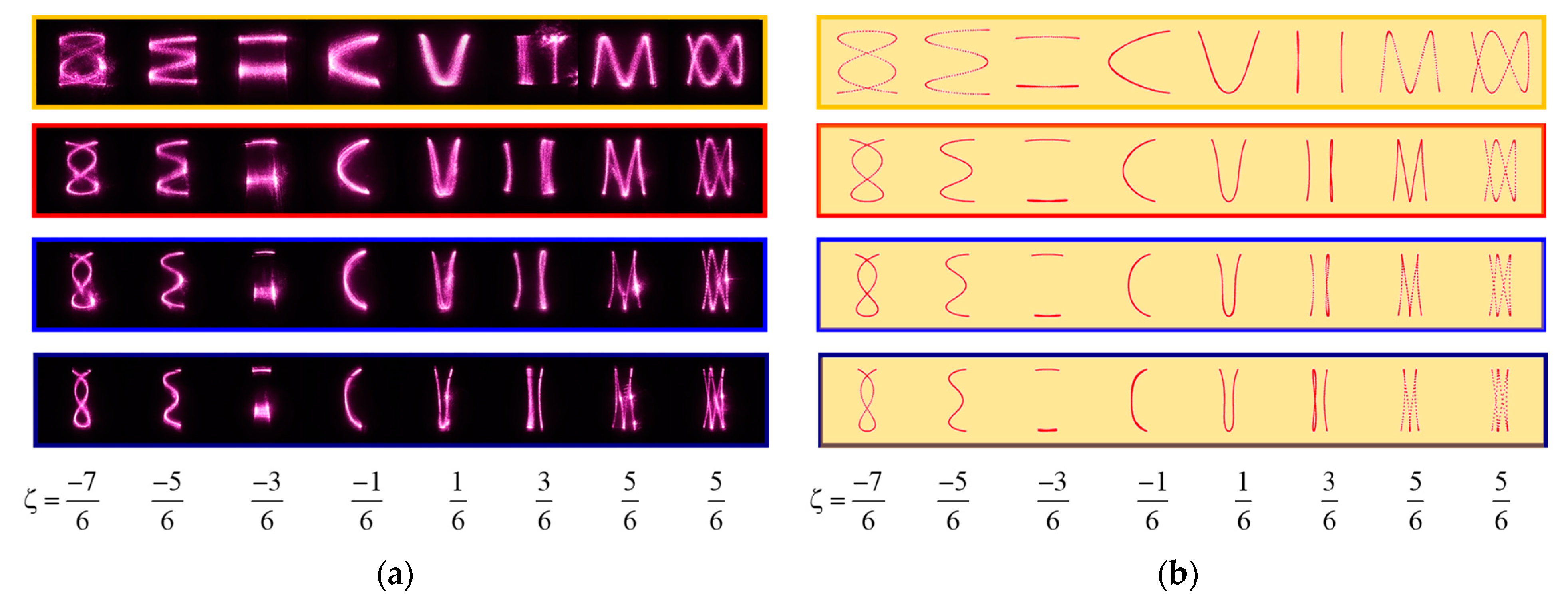
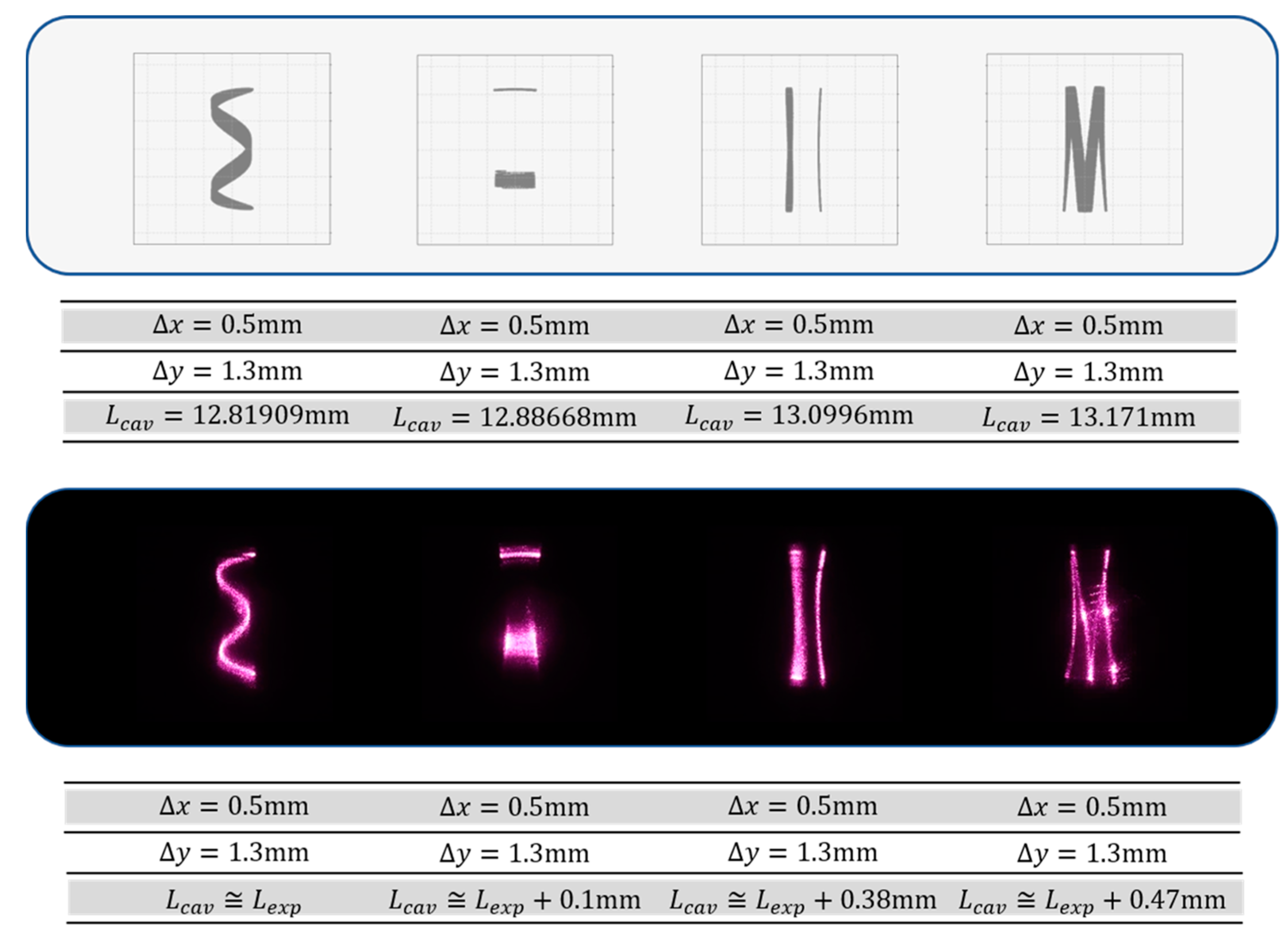
2.3. The Emergence and Distortion of Lissajous-like Structural Laser Mode

Without considering the birefringent effect of the gain medium, it can be concluded that $\mathsf{\theta }/2\mathsf{\pi }={\sin }^{-1}\left(\sqrt{{L_c/R}_c}\right)/\mathsf{\pi }$ in Equation (3). It is well known as the ratio of transverse mode spacing $\mathrm{\Delta }{f}_T$ to longitudinal mode spacing $\mathrm{\Delta }{f}_L$ in laser physics.

$$\frac{\mathsf{\theta }}{2\mathsf{\pi }}=\frac{\mathrm{\Delta }{f}_T}{\mathrm{\Delta }{f}_L}=\frac{1}{\mathsf{\pi }}{\sin }^{-1}\left(\sqrt{\frac{L_c}{R_c}}\right),$$

(11)

where $R_c$ is the radius of curvature of the concave mirror and $L_c$ is the effective cavity length [8,14]. When the right-hand side of Equation (11), $\sqrt{L_c/R_c}$, leads to a simple rational number, $P/Q$, the optical ray inside the laser cavity forms a periodic trajectory with $Q$ round reflections, where $P$ and $Q$ are mutually prime. The ratio of transverse to longitudinal mode spacing for $L_c=L_{P/Q}+\delta L$ can be simplified as

$${\left.\frac{\mathrm{\Delta }{f}_T}{\mathrm{\Delta }{f}_L}\right|}_{L_{P/Q}+\delta L}={\left.\frac{\mathrm{\Delta }{f}_T}{\mathrm{\Delta }{f}_L}\right|}_{L_{P/Q}}+\delta L\frac{d}{dL}\left({\left.\frac{\mathrm{\Delta }{f}_T}{\mathrm{\Delta }{f}_L}\right|}_{L_{P/Q}}\right),$$

(12)

$$\frac{d}{dL}\left(\frac{\mathrm{\Delta }{f}_T}{\mathrm{\Delta }{f}_L}\right)=\frac{1}{2\mathsf{\pi }\sqrt{L_c\left(R_c-L_c\right)}}.$$

(13)

Since ${\text{Nd:YVO}}_4$ crystals are positive uniaxial crystals with large birefringence, there is considerable astigmatism in the laser cavity. According to the experimental result in Figure 4 and Figure 5, the effective cavity length difference between x and y directions is approximately about $d=d_{crystal}·\left[1/n_e-1/\left(n_e+\delta n\right)\right]$. Considering Equations (11)–(13) and effective cavity length difference $d$, the mode spacing in the x and y directions can be given by

$$\frac{\mathrm{\Delta }{f}_{Tx}}{\mathrm{\Delta }{f}_L}=\frac{P}{Q}+\frac{\left[\delta L-\left(d/2\right)\right]}{2\mathsf{\pi }{z}_{Rx}},$$

(14)

$$\frac{\mathrm{\Delta }{f}_{Ty}}{\mathrm{\Delta }{f}_L}=\frac{P}{Q}+\frac{\left[\delta L+\left(d/2\right)\right]}{2\mathsf{\pi }{z}_{Ry}},$$

(15)

where

$$z_{Rx}=\sqrt{\left[L_{P/Q}-\left(d/2\right)\right]\left[R_C-L_{P/Q}+\left(d/2\right)\right]},$$

(16)

$$z_{Ry}=\sqrt{\left[L_{P/Q}+\left(d/2\right)\right]\left[R_C-L_{P/Q}-\left(d/2\right)\right]}.$$

(17)

When the right-hand sides of Equations (14) and (15) satisfy these forms, $P/Q\left(1-q/M\right)$ and $P/Q\left(1+p/M\right)$, respectively, the optical ray inside the cavity forms a Lissajous-like structure with indices $\left(p,q\right)$ that satisfy

$$\frac{z_{Ry}\left[\delta L-\left(d/2\right)\right]}{z_{Rx}\left[\delta L+\left(d/2\right)\right]}=\frac{-q}{p}.$$

(18)

In the degenerate cavity, there is a linear relationship between cavity length and 3D Lissajous-like structural laser modes [13], and the slope of the line can be confirmed as the effective cavity length difference, $d=d_{crystal}·\left[1/n_e-1/\left(n_e+\delta n\right)\right]$.

$$L_{P/Q;\zeta }=L_{P/Q}+\delta L,$$

(19)

$$\delta L=\frac{d}{2}\left(\frac{p{z}_{Ry}-q{z}_{Rx}}{p{z}_{Ry}+q{z}_{Rx}}\right)=\zeta d,$$

(20)

where $L_{P/Q;\zeta }$ indicates the cavity length observing the 3D Lissajous-like structural laser mode, and integers $p$ and $q$ satisfy $p+q=nQ$ with $n$ as a positive integer. Figure 9 shows the experimental and theoretical results for $L_{P/Q;\zeta }$ with $P/Q=1/3$ and $2/5$ versus $\zeta$. The vertical coordinates of the symbols in Figure 9a are experimental values of cavity lengths $L_{cav}$ for the observation of the Lissajous-like structural laser mode with indices $\left(p,q\right)$, and their horizontal coordinates are calculated from Equation (20). The output powers for all observed 3D Lissajous-like structural laser modes are found to be approximately 180 mW at an incident pumped power of 5.0 W. The best match for theoretical calculations to experimental results can be seen to be approximately d = 1.15, 0.63 mm. Figure 9b,c shows the observed Lissajous-like structural laser modes in the experiment and numerical results calculated using $x_s=A\cos \left[\left(2\mathsf{\pi }sP/Q\right)\left(1-q/M\right)\right]$ and $y_s=B\cos \left[\left(2\mathsf{\pi }sP/Q\right)\left(1+p/M\right)\right]$ with $P/Q=1/3$ and $2/5$, $s=0,1,2\cdots MQ-1$, $A=B=10$, $M=400$ and indices $\left(p,q\right)$.

However, in the experiments, the slope of the line and the Lissajous-like structural laser mode undergo slight changes and distortion in different off-axis pumping conditions; Figure 10. With the help of the 3D ray tracing model, all theoretical patterns can be seen to agree very well with the experimental patterns; Figure 11. For convenience, we simplify the 3D ray tracing model into the ABCD matrix in the discussion below.

3. Adjusted ABCD Matrix for Laser Cavity

ABCD Matrix for a Round Trip

The conventional ABCD matrix can be used for 2D separable trajectories. Here, we proposed a modified method for 3D ray tracing based on the adjusted ABCD matrix. This proposed method can be used to comprehend the origin of the distorted Lissajous modes. In the 2D situation, we make the following assumptions: we assume $v_z\gg v_x$, only consider the first two terms of the Taylor expansion for ${\sin }^{-1}\left(\tilde{x}\right)=\tilde{x}+{\tilde{x}}^3/6+3{\tilde{x}}^5/40+\cdots$, and ignore the ray path difference in different locations and propagation directions. We can obtain the adjusted ABCD matrix for a round trip.

$$\left(\begin{array}{cc}1& L\\ 0& 1\end{array}\right)\left(\begin{array}{cc}1& 0\\ \frac{-2}{x}\left(\tilde{x}+\frac{{\tilde{x}}^3}{6}\right)& 1\end{array}\right)\left(\begin{array}{cc}1& L\\ 0& 1\end{array}\right)=M\left(\tilde{x}\right).$$

(21)

Then, the adjusted ABCD matrix for a round trip considering a birefringence crystal is shown below, where $\tilde{x}=x/R$ in the matrix. In addition, the adjusted y-direction ABCD matrix can easily be determined by changing refractive index $n_e$ to $n_e+\delta n$.

$$\left(\begin{array}{cc}1& d_{crystal}\\ 0& 1\end{array}\right)\left(\begin{array}{cc}1& 0\\ 0& 1/n_e\end{array}\right)M\left(\tilde{x}\right)\left(\begin{array}{cc}1& 0\\ 0& n_e/1\end{array}\right)\left(\begin{array}{cc}1& d_{crystal}\\ 0& 1\end{array}\right)=\left(\begin{array}{cc}{A}_x\left(\tilde{x}\right)& B_x\left(\tilde{x}\right)\\ C_x\left(\tilde{x}\right)& D_x\left(\tilde{x}\right)\end{array}\right).$$

(22)

To use the adjusted ABCD matrix, the easiest method to obtain the ray location in Equation (22) is to use the iterative method to calculate the ray trajectory, as shown in the equation below.

$$\left(\begin{array}{cc}{A}_x\left(\tilde{x}\right)& B_x\left(\tilde{x}\right)\\ C_x\left(\tilde{x}\right)& D_x\left(\tilde{x}\right)\end{array}\right)\left(\begin{array}{c}{x}_n\\ {\mathsf{\theta }}_n\end{array}\right)=\left(\begin{array}{c}{x}_{n+1}\\ {\mathsf{\theta }}_{n+1}\end{array}\right).$$

(23)

In a 3D situation, we need to calculate the ray trajectory in the x direction and the y direction, respectively, then consider both the x component and the y component to calculate the reflection by a concave mirror using the following transformation matrix:

$$\left(\begin{array}{c}{\mathsf{\theta }}_{\mathsf{\rho }}\\ {\mathsf{\theta }}_{\mathsf{\varphi }}\end{array}\right)=\frac{1}{\mathsf{\rho }}\left(\begin{array}{cc}x& y\\ -y& x\end{array}\right)\left(\begin{array}{c}{\mathsf{\theta }}_x\\ {\mathsf{\theta }}_y\end{array}\right).$$

(24)

Then, the velocity vectors related to ${\mathsf{\theta }}_{\mathsf{\rho }}$ and ${\mathsf{\theta }}_{\mathsf{\varphi }}$ need to be reprojected back into Cartesian coordinates as

$$\left(\begin{array}{c}{\mathsf{\theta }}_x\\ {\mathsf{\theta }}_y\end{array}\right)=\frac{1}{\mathsf{\rho }}\left(\begin{array}{cc}x& -y\\ y& x\end{array}\right)\left(\begin{array}{c}{\mathsf{\theta }}_{\mathsf{\rho }}\\ {\mathsf{\theta }}_{\mathsf{\varphi }}\end{array}\right).$$

(25)

Based on the reprojection, the aberration problem of the concave mirrors in large off-axis pumping can be well considered. More importantly, the connection between the aberration of the concave mirror and the distortion of the Lissajous modes can be clearly comprehended. This proposed method can be used. The overall steps for a complete round trip are given in Figure 12.

Given different 2D off-axis pumping conditions and cavity lengths, we can obtain the ray trajectory distribution by the 3D adjusted ABCD matrix. Figure 13 shows the emergence of the distortion for the 2D HG mode through the off-axis pump increasing, and Figure 14 shows the various types of distortion Lissajous-like structural laser modes that can be observed in both numerical calculations and experiments.

4. Conclusions

In this paper, we discuss how the 3D Lissajous-like structural laser mode forms, starting at the geometric optics and considering the gain medium ${\text{Nd:YVO}}_4$. Instead of using the refractive index ellipsoid, it is more likely that the refractive index is ${\stackrel{\rightharpoonup }{n}}_c=n_e{\widehat{a}}_x+\left(n_e+\delta n\right){\widehat{a}}_y$ and $\delta n\cong 0.54$, and this refractive index difference determines the Lissajous-like structural laser modes. Combining the factor of the concave mirror and the birefringence crystal, we finally complete the 3D ray tracing model. Furthermore, we simplify this model into an adjusted ABCD matrix, which can confirm the rotation of the ray trajectory. The emergence and distortion of the Lissajous-like structural laser mode can be simulated with the adjusted ABCD matrix and iterative calculation. We believe that this trajectory calculation model provides a good research direction for studies related to high-order modes, structured laser beams, and vortex light within the laser resonant cavity.

References

1. Feng, S.; Winful, H.G. Physical origin of the Gouy phase shift. Opt. Lett. 2001, 26, 485–487. [Google Scholar] [CrossRef] [PubMed]
2. Hamazaki, J.; Mineta, Y.; Oka, K.; Morita, R. Direct observation of Gouy phase shift in a propagating optical vortex. Opt. Express 2006, 14, 8382–8392. [Google Scholar] [CrossRef] [PubMed]
3. Marte, M.A.; Stenholm, S. Paraxial light and atom optics: The optical Schrödinger equation and beyond. Phys. Rev. A 1997, 56, 2940. [Google Scholar] [CrossRef]
4. Paré, C.; Gagnon, L.; Bélanger, P.A. Aspherical laser resonators: An analogy with quantum mechanics. Phys. Rev. A 1992, 46, 4150. [Google Scholar] [CrossRef] [PubMed]
5. Moran, J.; Hussin, V. Coherent states for the isotropic and anisotropic 2D harmonic oscillators. Quantum Rep. 2019, 1, 260–270. [Google Scholar] [CrossRef]
6. Kogelnik, H.; Li, T. Laser beams and resonators. Appl. Opt. 1966, 5, 1550–1567. [Google Scholar] [CrossRef]
7. Senatsky, Y.; Bisson, J.F.; Li, J.; Shirakawa, A.; Thirugnanasambandam, M.; Ueda, K.I. Laguerre-Gaussian modes selection in diode-pumped solid-state lasers. Opt. Rev. 2012, 19, 201–221. [Google Scholar] [CrossRef]
8. Barré, N.; Romanelli, M.; Lebental, M.; Brunel, M. Waves and rays in plano-concave laser cavities: I. Geometric modes in the paraxial approximation. Eur. J. Phys. 2017, 38, 034010. [Google Scholar]
9. Liang, H.C.; Lin, H.Y. Generation of resonant geometric modes from off-axis pumped degenerate cavity Nd:YVO4 lasers with external mode converters. Opt. Lett. 2020, 45, 2307–2310. [Google Scholar] [CrossRef]
10. Visser, J.; Zelders, N.J.; Nienhuis, G. Wave description of geometric modes of a resonator. JOSA A 2005, 22, 1559–1566. [Google Scholar] [CrossRef]
11. Dingjan, J.; Van Exter, M.P.; Woerdman, J.P. Geometric modes in a single-frequency Nd:YVO4 laser. Opt. Commun. 2001, 188, 345–351. [Google Scholar] [CrossRef]
12. Lu, T.H.; He, C.H. Generating orthogonally circular polarized states embedded in nonplanar geometric beams. Opt. Express 2015, 23, 20876–20883. [Google Scholar] [CrossRef] [PubMed]
13. Zheng, X.L.; Hsieh, M.X.; Chen, Y.F. Quantifying the emergence of structured laser beams relevant to Lissajous parametric surfaces. Opt. Lett. 2022, 47, 2518–2521. [Google Scholar] [CrossRef] [PubMed]
14. Tung, J.C.; Tuan, P.H.; Liang, H.C.; Huang, K.F.; Chen, Y.F. Fractal frequency spectrum in laser resonators and three-dimensional geometric topology of optical coherent waves. Phys. Rev. A 2016, 94, 023811. [Google Scholar] [CrossRef]
15. Tuan, P.H.; Cheng, K.T.; Cheng, Y.Z. Generating high-power Lissajous structured modes and trochoidal vortex beams by an off-axis end-pumped Nd:YVO4 laser with astigmatic transformation. Opt. Express 2021, 29, 22957–22965. [Google Scholar] [CrossRef] [PubMed]
16. Lu, T.H.; Lin, Y.C.; Chen, Y.F.; Huang, K.F. Three-dimensional coherent optical waves localized on trochoidal parametric surfaces. Phys. Rev. Lett. 2008, 101, 233901. [Google Scholar] [CrossRef] [PubMed]
17. Hu, A.; Lei, J.; Chen, P.; Wang, Y.; Li, S. Numerical investigation on the generation of high-order Laguerre–Gaussian beams in end-pumped solid-state lasers by introducing loss control. Appl. Opt. 2014, 53, 7845–7853. [Google Scholar] [CrossRef] [PubMed]
18. Cui, R.; Dong, L.; Wu, H.; Li, S.; Yin, X.; Zhang, L.; Ma, W.; Yin, W.; Tittel, F.K. Calculation model of dense spot pattern multi-pass cells based on a spherical mirror aberration. Opt. Lett. 2019, 44, 1108–1111. [Google Scholar] [CrossRef] [PubMed]
19. Senatsky, Y.; Bisson, J.F.; Shelobolin, A.; Shirakawa, A.; Ueda, K. Circular modes selection in Yb:YAG laser using an intracavity lens with spherical aberration. Laser Phys. 2009, 19, 911–918. [Google Scholar] [CrossRef]
20. Chao, S.L.; Forsyth, J.M. Properties of high-order transverse modes in astigmatic laser cavities. JOSA 1975, 65, 867–875. [Google Scholar] [CrossRef]
21. Chao, S.L. Astigmatic resonator for closed-cavity-mode filling enhancement. Appl. Opt. 1985, 24, 676–681. [Google Scholar] [CrossRef] [PubMed]
22. Chen, Y.F.; Tung, J.C.; Hsieh, M.X.; Hsieh, Y.H.; Liang, H.C.; Huang, K.F. Generalized wave-packet formulation with ray-wave connections for geometric modes in degenerate astigmatic laser resonators. Opt. Lett. 2019, 44, 5366–5369. [Google Scholar] [CrossRef] [PubMed]
Figure 1. Experimental setup for exciting the high-order mode of the laser pattern.
Photonics 11 00456 g001
Figure 2. Plotting the reflection ray path by a concave mirror of an R = 20 mm radius curvature, where θ R = sin 1 Δ x R , Δ x indicates the distance between the incident point and the center point of the mirror, ϕ and ϕ indicate the ray angle relative to a ^ z and a ^ z , respectively.
Photonics 11 00456 g002
Figure 3. (a) The three round-trip ray trajectories in specific cavity length L c a v (the distance between concave mirror and crystal); (b) The thirty round-trip ray trajectories in specific cavity length L c a v ; (c) The three hundred round-trip ray trajectories in specific cavity length L c a v .
Photonics 11 00456 g003
Figure 4. The use of the ray tracing model with refractive index n e f f x = n e in vertical polarization to quantize the periodic property. The above figure represents the simple periodic trajectories simulated by the ray tracing model and the bottom image illustrates several observed geometric modes in the a ^ x axis in the experiment.
Photonics 11 00456 g004
Figure 5. By comparing experiments data and simulation results, it can be noticed that the refractive index shows n e f f y = n e + 0.54 in vertical polarization. The following image illustrates several observed geometric modes in the a ^ y axis in the experiment.
Photonics 11 00456 g005
Figure 6. (a) To discuss the ray trajectory in the crystal, we need to consider the refraction in both the x-z plane and the y-z plane, respectively, in the 3D situation; (b) the displacement in the x-z plane.
Photonics 11 00456 g006
Figure 7. (a) To discuss the ray trajectory reflected by the concave mirror, we need to decompose the propagation direction into radius direction a ^ ρ and azimuthal direction a ^ ϕ ; (b) the decomposition in the x-y plane where v x y p l a n e indicates the velocity vector on the x-y plane.
Photonics 11 00456 g007
Figure 8. (a) The schematic of the end-side pumping with off-axis displacement; (b) The Lissajous-like trajectory inside the laser cavity is simulated using the 3D ray tracing model, and the trajectory changes in the rays from the laser cavity after leaving it during their free space propagation also agree with the experimental observation.
Photonics 11 00456 g008
Figure 9. (a) Experimental and theoretical results for L c a v versus ζ for the emergence of the Lissajous-like structural laser modes around L P / Q = 1 / 3 and L P / Q = 2 / 5 . (b) Lissajous-like structural laser modes observed in the experiment. (c) Lissajous parametric surfaces calculated using x s = A cos 2 π s P / Q 1 q / M and y s = B cos 2 π s P / Q 1 + p / M with P / Q = 1 / 3 and 2 / 5 , s = 0 , 1 , 2 M Q 1 , A = B = 10 , M = 400 and indices p , q .
Photonics 11 00456 g009
Figure 10. The points in the figure represent the cavity lengths corresponding to the Lissajous-like structural laser modes observed experimentally under different off-axis pumping conditions, and the lines represent the cavity lengths at which the Lissajous trajectories appear in the 3D ray tracing model under different off-axis pumping conditions.
Photonics 11 00456 g010
Figure 11. (a) The distortion Lissajous-like structural laser modes observed in the experiment; (b) the far field of the ray trajectories at the end side of crystal calculated using the 3D ray tracing model.
Photonics 11 00456 g011
Figure 12. The adjusted ABCD matrix for a round trip in the 3D laser cavity.
Photonics 11 00456 g012
Figure 13. Given cavity length L c a v and 2D off-axis pumping Δ x and Δ y , the far field of the ray trajectories at the end side of crystal calculated using the adjusted ABCD matrix are shown in the above figure. The lower row is the far field of the distortion 2D HG modes in the experiments.
Photonics 11 00456 g013
Figure 14. Given cavity length L c a v and 2D off-axis pump Δ x and Δ y , the far field of the ray trajectories at the end side of the crystal calculated using the adjusted ABCD matrix are shown in the above figure. The lower row is the far field of the distortion Lissajous-like structural laser modes observed in experiments with cavity lengths near L c a v .
Photonics 11 00456 g014
Disclaimer/Publisher’s Note: The statements, opinions and data contained in all publications are solely those of the individual author(s) and contributor(s) and not of MDPI and/or the editor(s). MDPI and/or the editor(s) disclaim responsibility for any injury to people or property resulting from any ideas, methods, instructions or products referred to in the content.