1. Introduction
In recent years, FSO communication has been used in commercial, military, and scientific applications, and it is emerging as a good candidate for next-generation broadband services, since it supports a large bandwidth and has a quick and inexpensive setup, an unlicensed spectrum, and excellent security [
1,
2,
3]. However, the effects of atmospheric turbulence can cause fading, leading to a sharp deterioration in the performance of FSO systems [
4,
5,
6,
7]. Therefore, it is of great significance to study the influence of atmospheric turbulence on the FSO systems.
To achieve this, laboratory simulations of atmospheric turbulence channels are required. Previous studies have tended to use numerical simulation methods to simulate atmospheric turbulence channels. Distributions such as lognormally, Gamma–Gamma, Malaga, and K have been considered as fading channel models [
8,
9,
10,
11,
12,
13]. However, these methods are not suitable for testing actual FSO systems.
In [
14], the authors used an atmospheric turbulence simulation pool to simulate the atmospheric channel. The atmospheric turbulence simulation pool was mainly composed of a cooler, a heater, a temperature detection unit, a feedback control unit, and a pool body. The device used the principle of airflow similarity to simulate atmospheric turbulence. The principle of airflow similarity states that two fluid vortices are dynamically similar, when the Reynolds number is equal, and the geometric boundary conditions are similar, even if there is a difference in velocity and size. Although the atmospheric turbulence simulation pool can simulate the effects of atmospheric channels, it cannot fully reproduce a specific atmospheric channel due to the physical conditions and the instability of atmospheric turbulence.
In [
15], the phase screen generation method was used to simulate light propagation through atmospheric turbulence. The phase screen generator using the Fast Fourier Transform-based method generated 1024 × 1024 phase screens at a rate of 285 phase screens per minute.
In [
16,
17,
18], liquid crystal spatial light modulators were used for atmospheric turbulence simulation devices. These devices successfully demonstrated the impact of different turbulence intensities on laser atmospheric transmission, providing flexible operational solutions for simulating atmospheric turbulence.
In [
19], the authors reported the development of an atmospheric turbulence simulator for imaging telescopes, which consisted of two point sources, a commercially available deformable mirror with a 12 × 12 actuator array, and two random phase plates. The results showed that the simulator simulated atmospheric disturbances with Fried parameters that ranged from 7 to 15 cm at 500 nm.
In this study, the design of an atmospheric turbulence simulation system for an FSO system is proposed. A variable optical attenuator (VOA) is used as the execution unit. To ensure the convenience of the system, it was designed to receive atmospheric turbulence data via an Ethernet port. The experiments show that such a system can provide repeatable atmospheric turbulence simulation with high precision.
The remainder of the paper is organized as follows. In
Section 2, the design of the atmospheric turbulence simulation system is given, and the method for measuring and recording atmospheric turbulence channels is also introduced. Numerical and experimental results are given in
Section 3. Finally, some concluding remarks are provided in
Section 4.
2. Atmospheric Turbulence Channel Model
When an optical wave propagates through an atmospheric channel, it experiences intensity fluctuations or scintillation. Scintillation is mainly caused by small temperature variations in the atmosphere, resulting in an index of refraction fluctuations [
20]. In order to facilitate the expression, a logarithmic normal distribution fading channel that performs well in weak turbulence regions was used to test the system in this work. So, the probability density function (PDF) of the atmospheric turbulence induced fading is given as
where
σR2 is the Rytov variance. For a plane wave it can be written as
where
Cn2 is the atmospheric structure constant,
k = 2π/
λ is the wave number, and
L is the propagation distance. For an FSO system near the ground, the atmospheric structure constant varies from 10
−17 m
−2/3 to 10
−13 m
−2/3, according to the atmospheric turbulence conditions [
21]. The turbulent regime in the atmosphere is weak, moderate, strong, and extremely strong when
σR2 is <<1, ~1, >1, and >>1, respectively [
22].
Apart from the logarithmic normal distribution model, the Gamma–Gamma distribution model that is valid for all turbulence regimes was also used to process the experimental results. The PDF of the Gamma–Gamma distribution model is given as
where
stands for the modified Bessel function of the second kind of order
v, and
represents the Gamma function. For a plane wave, the parameters
and
can be approximately written as
3. Generation of Atmospheric Turbulence Channel Data
3.1. Measurement and Recording of Atmospheric Turbulence Channels
In order to simulate the actual atmospheric turbulence channels, measurement and recording are required.
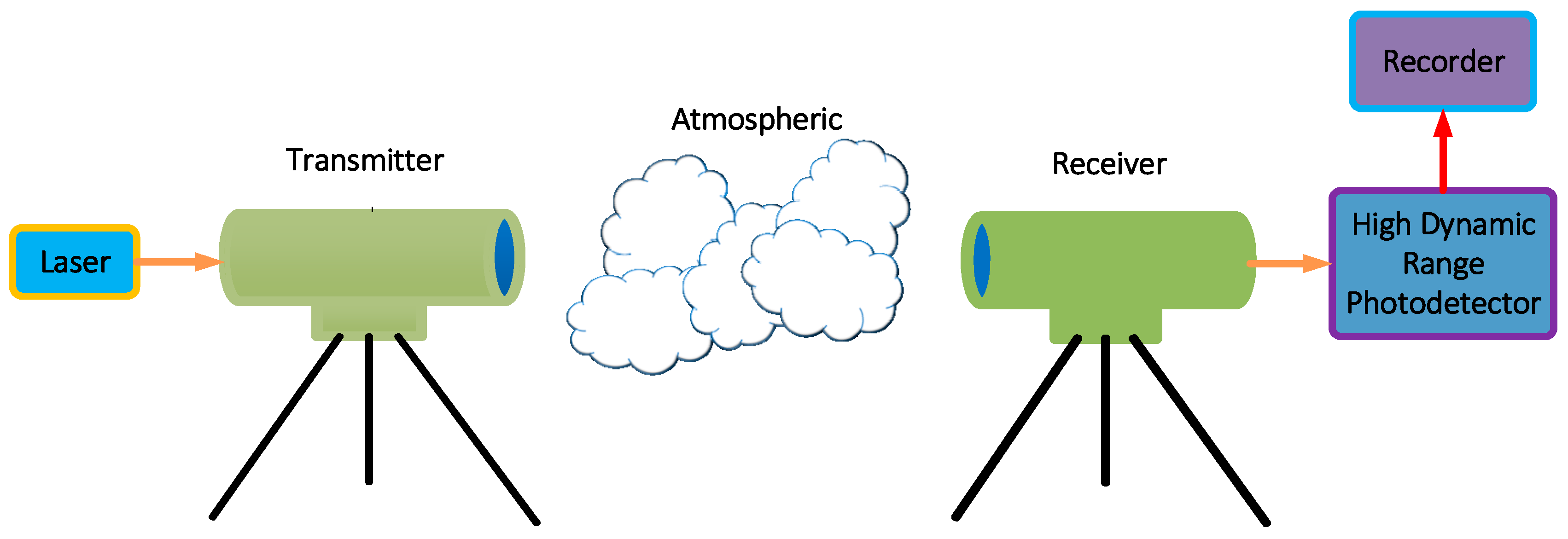
Figure 1 shows the schematic diagram of the system for measuring and recording atmospheric turbulence channel data. It consists of a laser, a transmitter, a receiver, a high dynamic range photodetector, a recorder, and an atmospheric channel. As shown in the figure, the composition of the system is similar to that of the FSO communication system. The atmospheric turbulence measurement and recording system works as follows: First, a continuous laser signal is sent to the atmospheric turbulence channel at the transmitter. Then, a high dynamic range photodetector is used to convert the received optical signal into an electrical signal. After that, the electrical signal is processed and stored in a local file. It should be noted that in order to ensure that the measured data can be adapted to the FSO system, the optical parameters of the transmitter and receiver must be set the same as the FSO system to be tested.
3.2. Generation of Atmospheric Turbulence Channel Data Using Atmospheric Channel Models
Apart from utilizing actual atmospheric turbulence channel data obtained through measurements and recordings, the system can also simulate atmospheric turbulence channels using data generated by atmospheric channel models with different FSO link lengths, turbulence strength, receiver characteristics, etc. This allows the system to emulate the behavior of different channels with different atmospheric conditions in the laboratory.
4. Atmospheric Turbulence Simulation System
After obtaining the data of the atmospheric turbulence channel, the atmospheric turbulence simulation system was used to simulate the channel according to the data recorded in the local file.
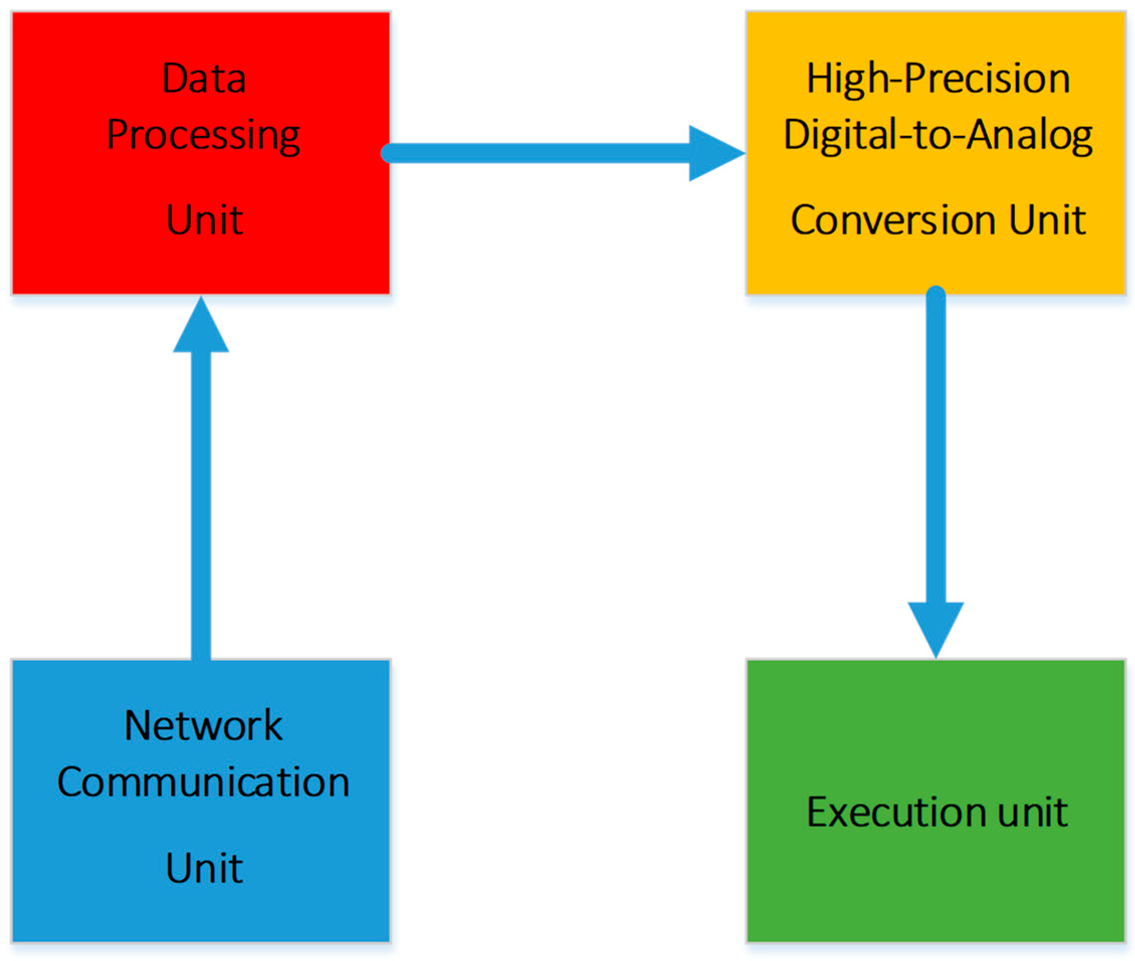
Figure 2 shows the architecture of the system. As shown in the figure, the device is composed of four units: network communication unit, data processing unit, high-precision digital-to-analog (DA) conversion unit, and execution unit. A Wiznet W5300 chip was used as the TCP/IP embedded Ethernet controller in the network communication unit. The TCP/IP protocol utilizes methods such as checksum, serial number/acknowledgment response, timeout retransmission, maximum message length, and sliding window control to achieve reliable transmission, which ensures the integrity and reliability of the transmitted channel data. For the data processing unit, an Intel Altera Cyclone II field programmable gate array (FPGA) chip was used to control the network communication unit and the high-precision DA conversion unit. A DAC7821 12-bit current output digital-to-analog converter with a large signal multiplying bandwidth of 10 MHz from Texas Instruments was used in the high-precision DA conversion unit. In order to simulate the deep fading in atmospheric turbulence channels, an SCVOA-B-C VOA from Accelink was used in the execution unit, which has a high executable dynamic range of 30 dB and an execution rate of 1 MHz. The composition of the system ensures that it has a dynamic execution range of 30 dB and an execution rate of 1 MHz, while also having an execution accuracy of over 0.1 dB.
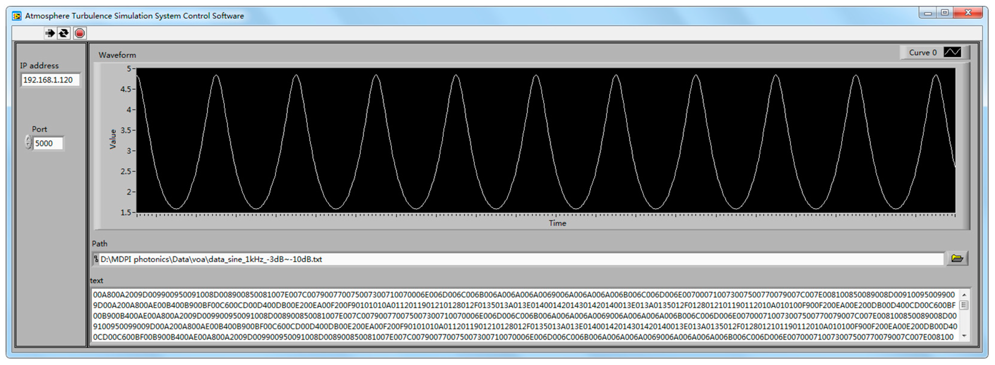
Figure 3 shows the interface of the version 1.0 control software for the atmospheric turbulence simulation system. The buttons in the upper left corner of the software are used to control the running and stopping of the software. The IP address and port number of the system can be entered through the editing box on the left side of the software. The path editing box is used to input the local path of the target channel data file. The display bar below the path editing bar is used to display the currently sent data. The waveform for the sending data is displayed in the waveform display area above the path editing bar.
The working process of the atmospheric turbulence simulation system is as follows: Firstly, the software on the host computer reads the atmospheric channel data from the local file and sends them to the atmospheric turbulence simulation system through the local area network. Then, the atmospheric turbulence simulation system analyzes and processes the data and converts them into executable data for the high-precision DA conversion unit. After that, the data are converted into an analog signal by the high-precision DA conversion unit and sent into the drive circuit in the execution unit. Finally, the driver circuit drives the VOA to simulate the recorded atmospheric turbulence channel.
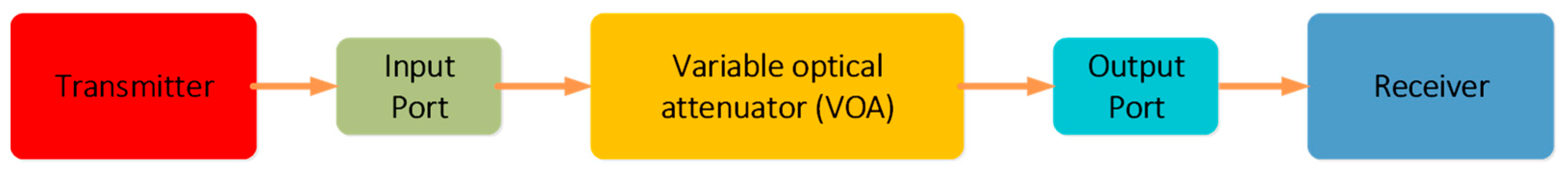
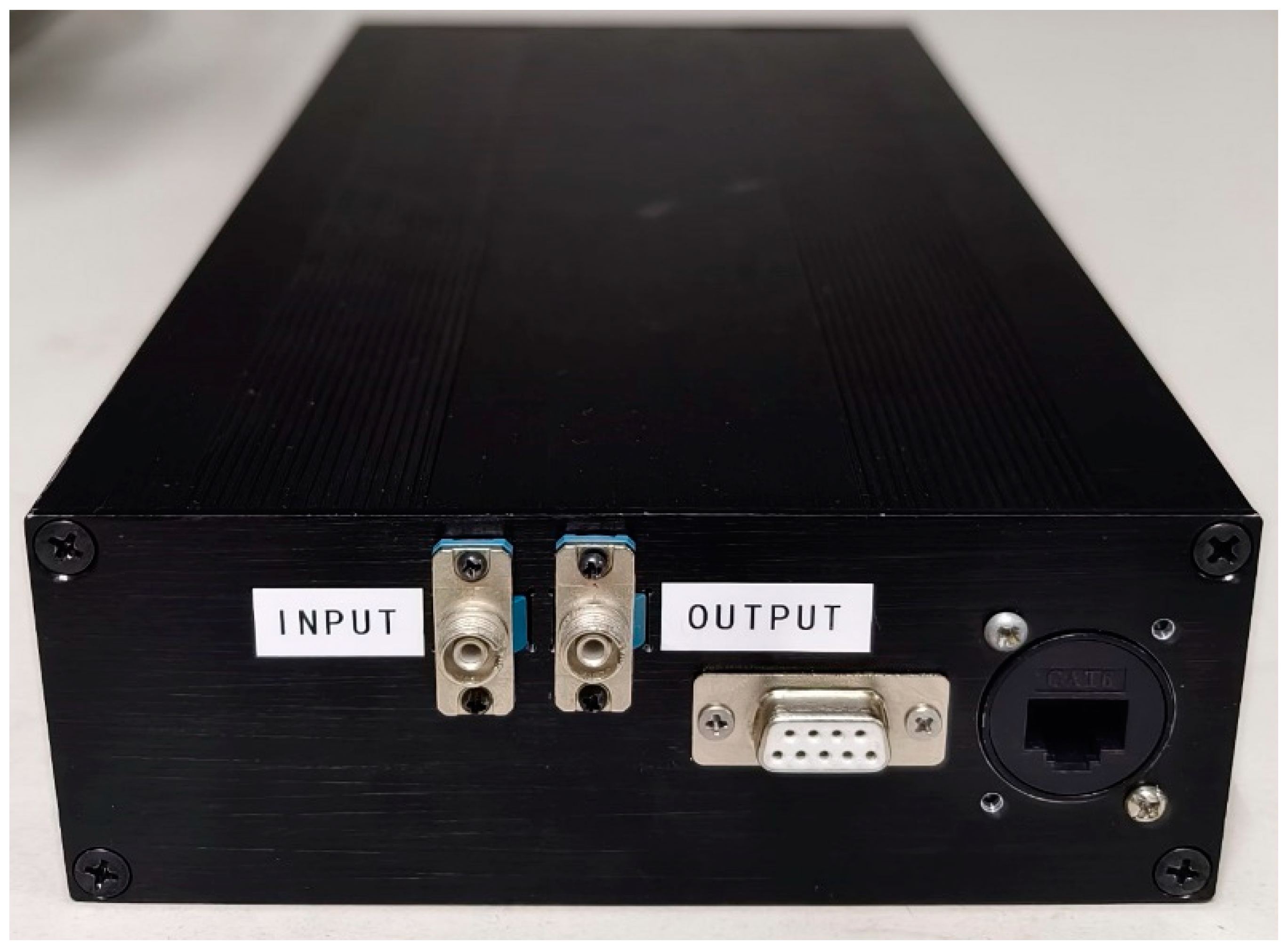
As shown in
Figure 4, two FC/PC single-mode fiber interfaces are used as the input port and output port for the optical signals. The optical path of the atmospheric turbulence simulation system during operation is plotted in
Figure 5. Firstly, the output optical signal of the FSO system transmitter to be tested is transmitted through optical fibers to the input port of the proposed system. Then, the VOA after the input port processes the optical signal based on the received channel data. Finally, the optical signal is sent to the output port and received by the receiver through optical fibers.
The atmospheric turbulence simulation system operates at a voltage of 220 V. The working frequency band of the system is the C-band. In addition, the reliable TCP/IP protocol is used for communication, which is plug-and-play and ensures the convenience and versatility of the system.
5. Numerical and Experimental Results
5.1. Experimental Setup
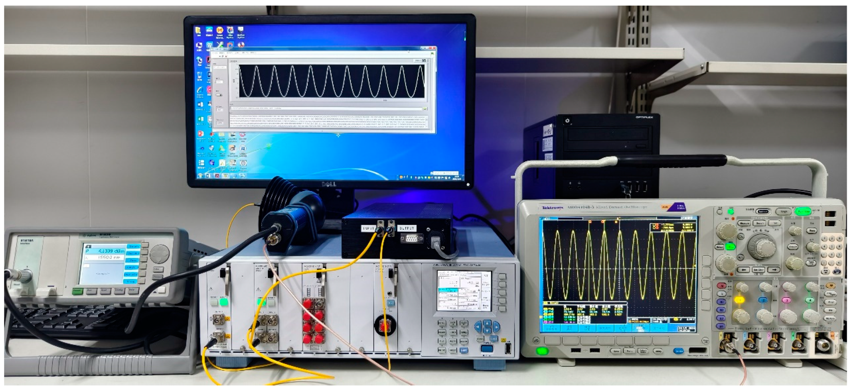
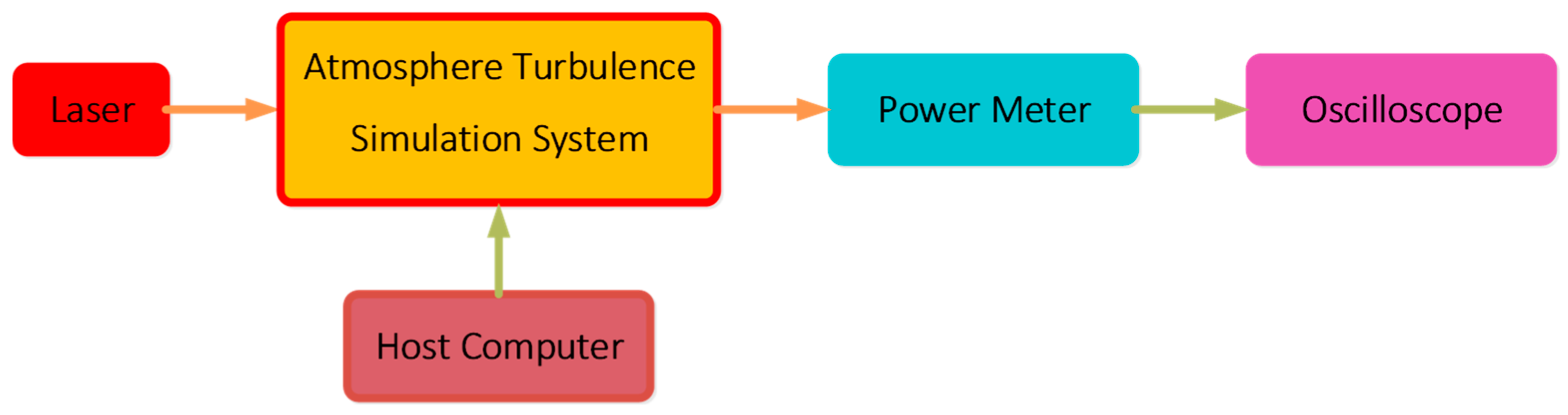
The experiments were carried out to investigate the performance of the proposed system. The block diagram and the photo of the experimental setup are shown in
Figure 6 and
Figure 7, respectively. The AQ2200-132 grid TLS module of the Yokogawa AQ2212 frame controller (Yokogawa Electric Corporation, Tokyo, Japan) was used as the laser source. The output of the laser source was connected to the input of the atmospheric turbulence simulation system. The system simulated the atmospheric turbulent fading channels based on the data sent by the host computer. The output of the system was connected to an Agilent 8163B optical power meter (Agilent Technologies, Santa Clara, CA, USA). Finally, the analog signal output by the optical power meter was fed into an oscilloscope. The power of the laser source was set at 11 dBm during the experiments.
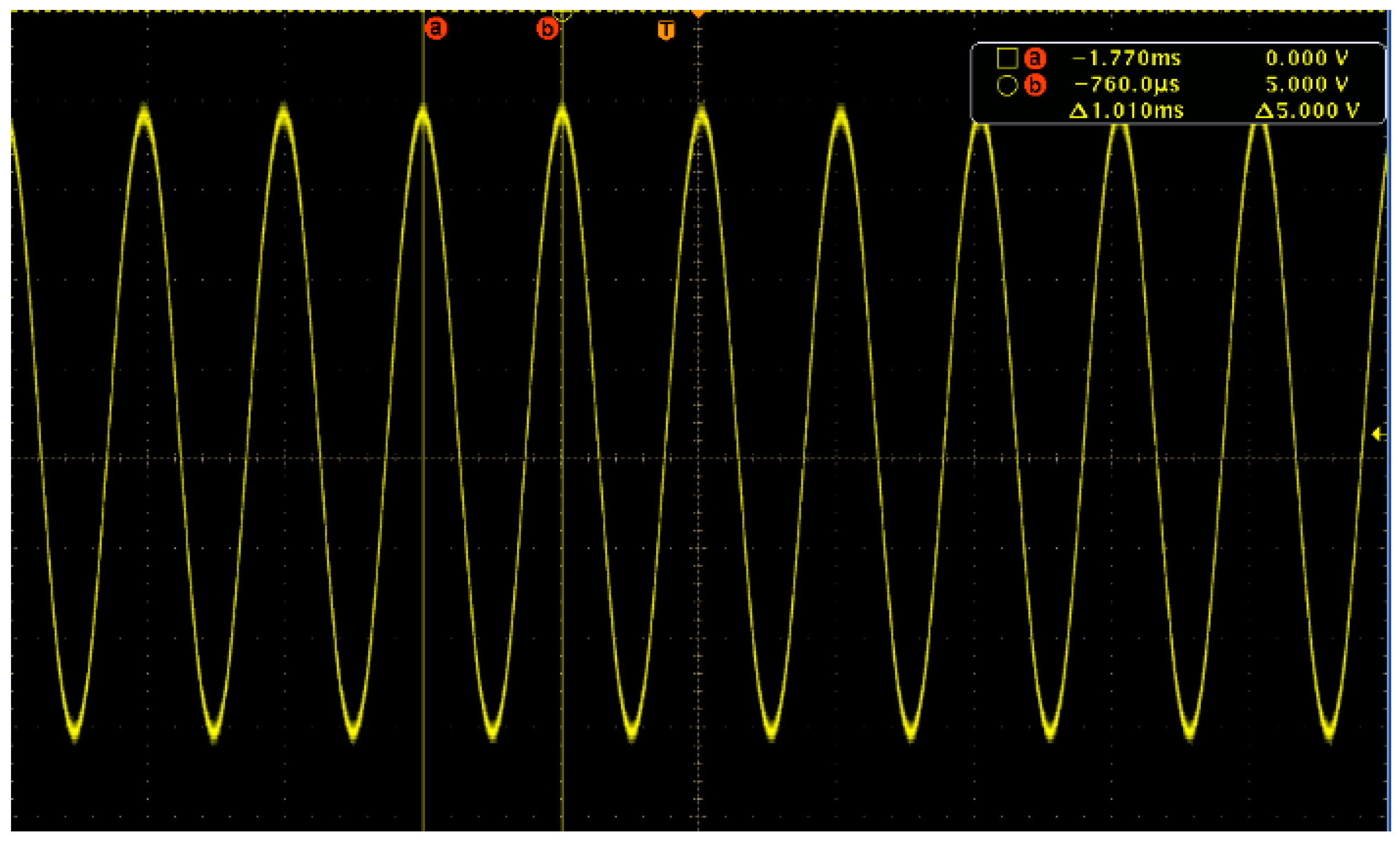
In order to test the system, a data file for the sine wave attenuation channel with a dynamic range of 7 dB and a frequency of 1 kHz was written and sent to the atmospheric turbulence simulation system through the control software. As shown in
Figure 8, the atmospheric turbulence simulation system accurately simulated the sine wave attenuation channel in the data file.
5.2. Experimental Results of the Data Generated Using Atmospheric Channel Models
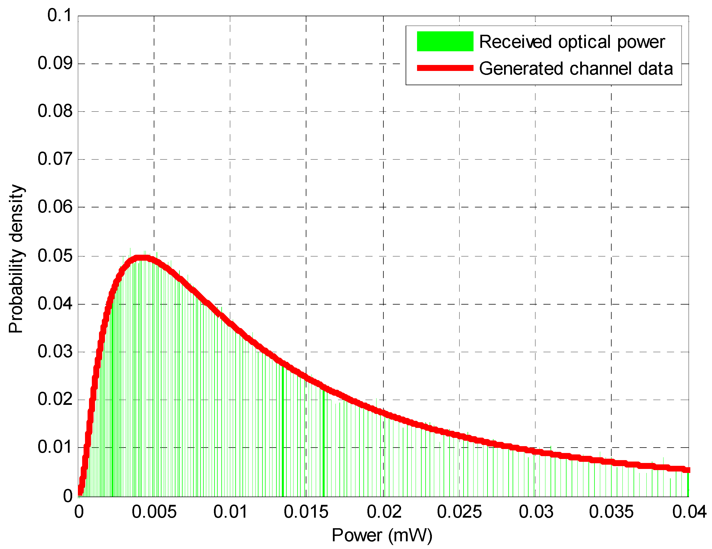
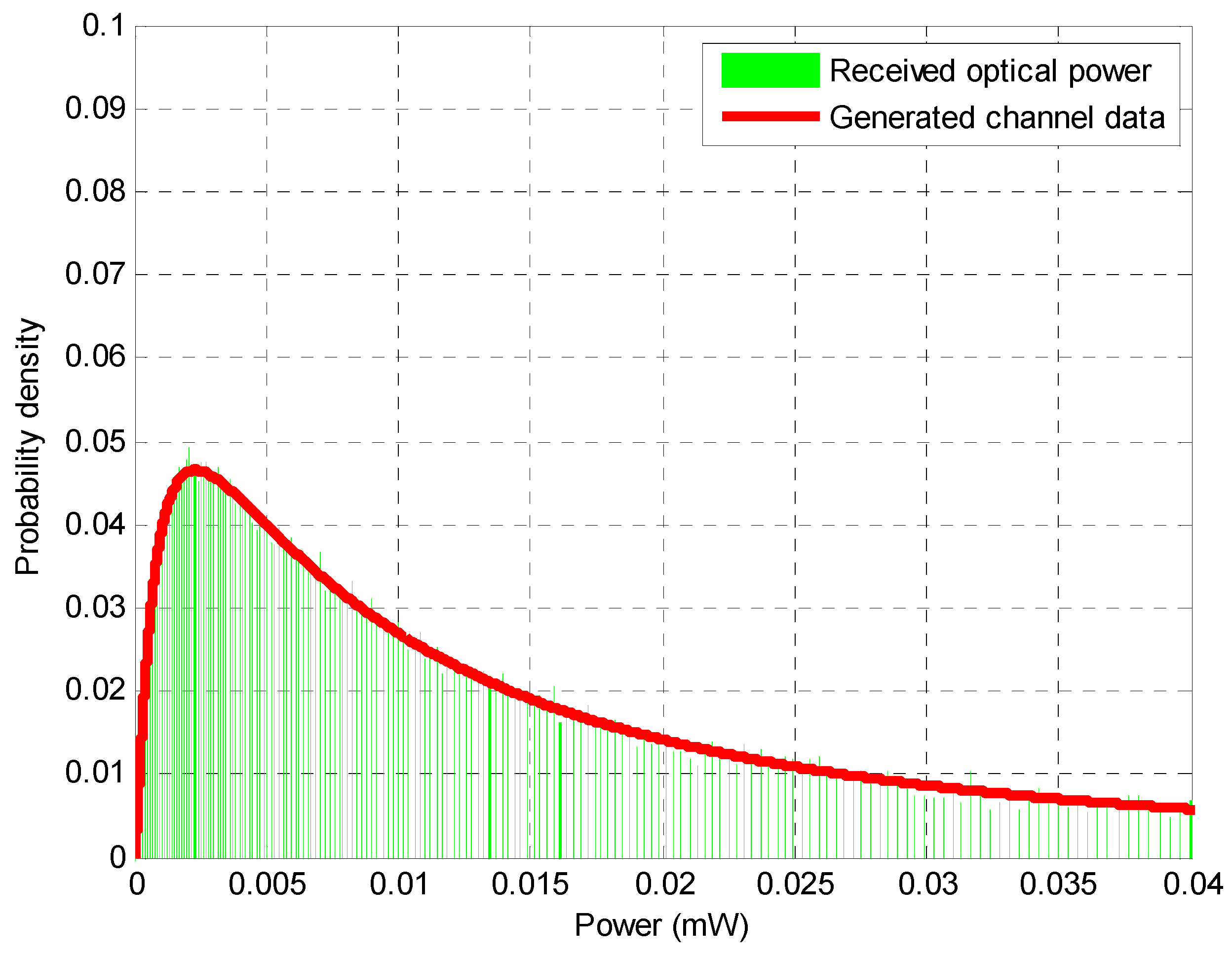
In order to verify the ability of the system to emulate the behavior of different channels under different atmospheric conditions in the laboratory, several sets of independent lognormal turbulence channel data with a length of 5 × 10
5 were generated by MATLAB software (version R2024a), according to the parameters given in
Table 1. It should be noted that when the receiver aperture is sufficiently large, it can have a significant impact on fading through aperture averaging. However, many FSO communication systems have relatively small receiver apertures, which can be considered as “point apertures” [
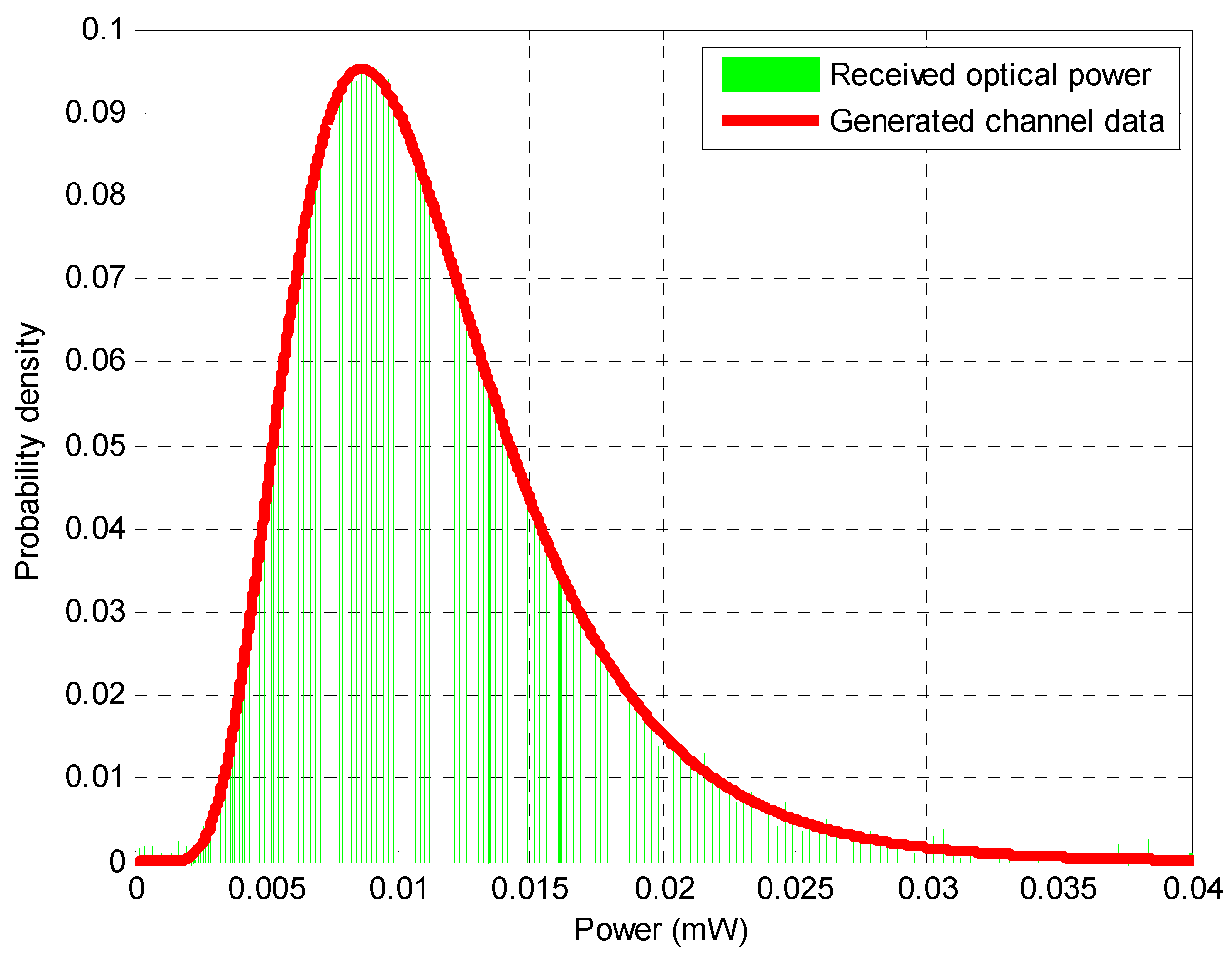
23]. Therefore, for the convenience of description, the receiver aperture was considered as the “point aperture” in the process of generating channel data. Then, the generated data were sent to the system by the control software on the host computer. The results of the experiment are shown in
Figure 9,
Figure 10 and
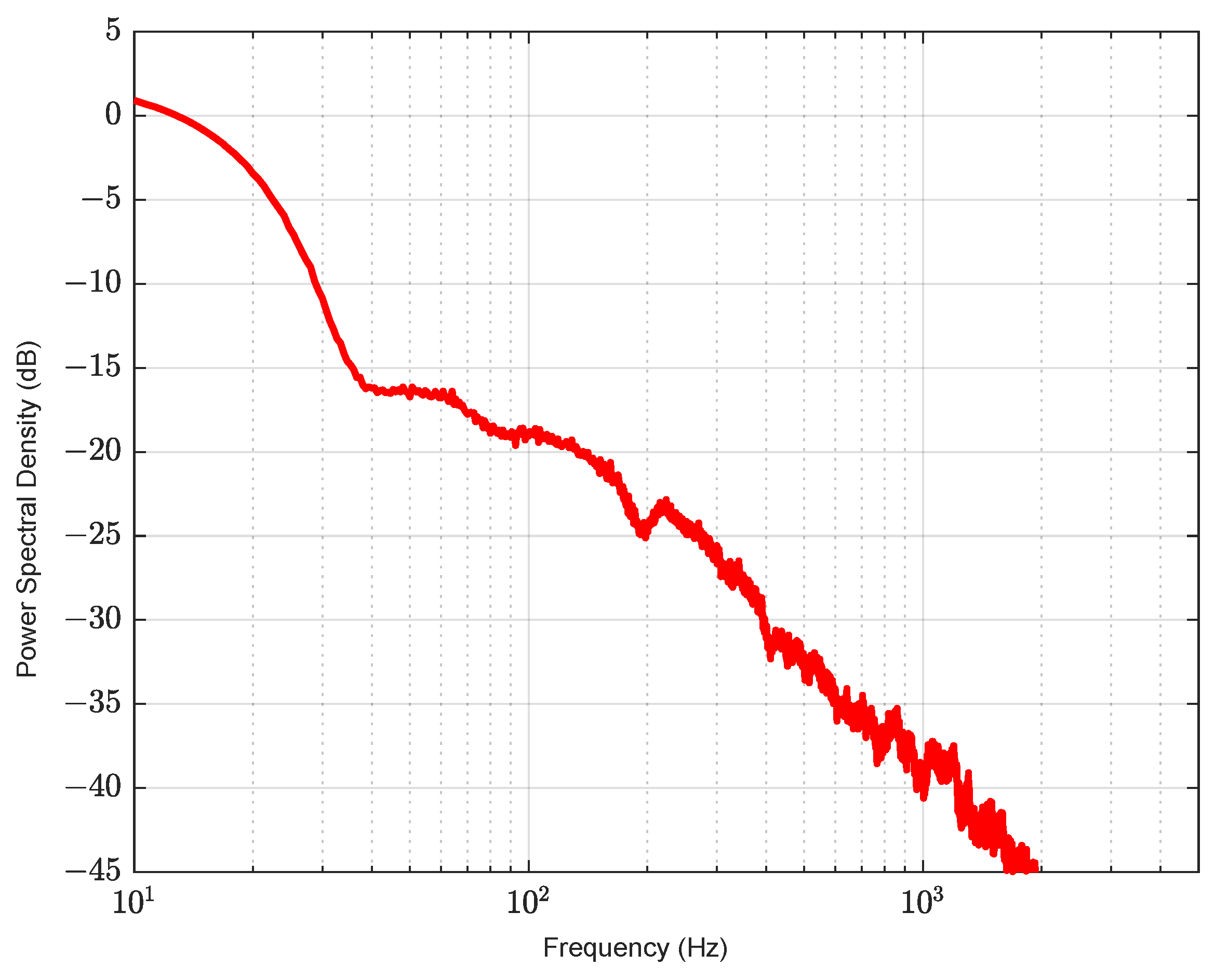
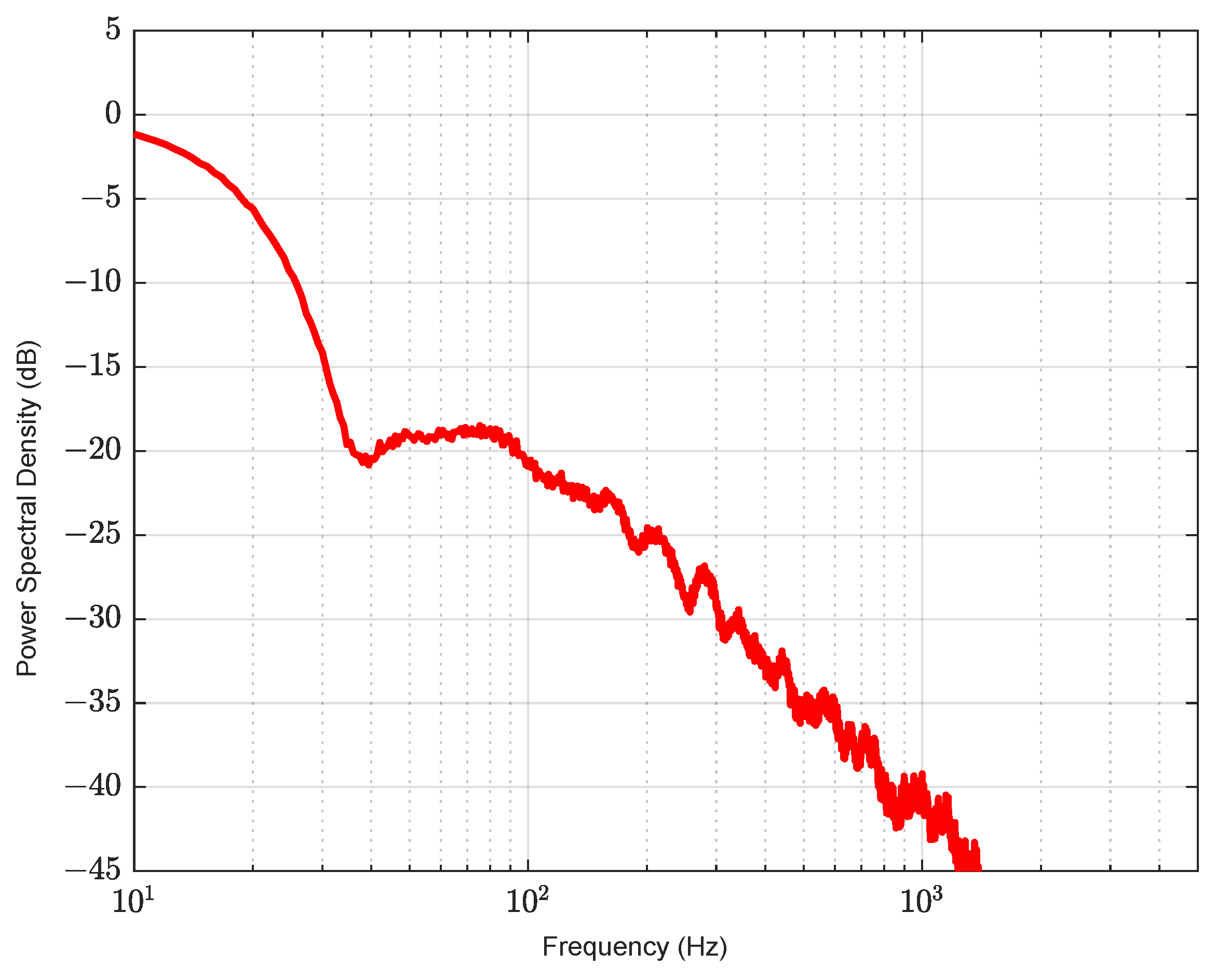
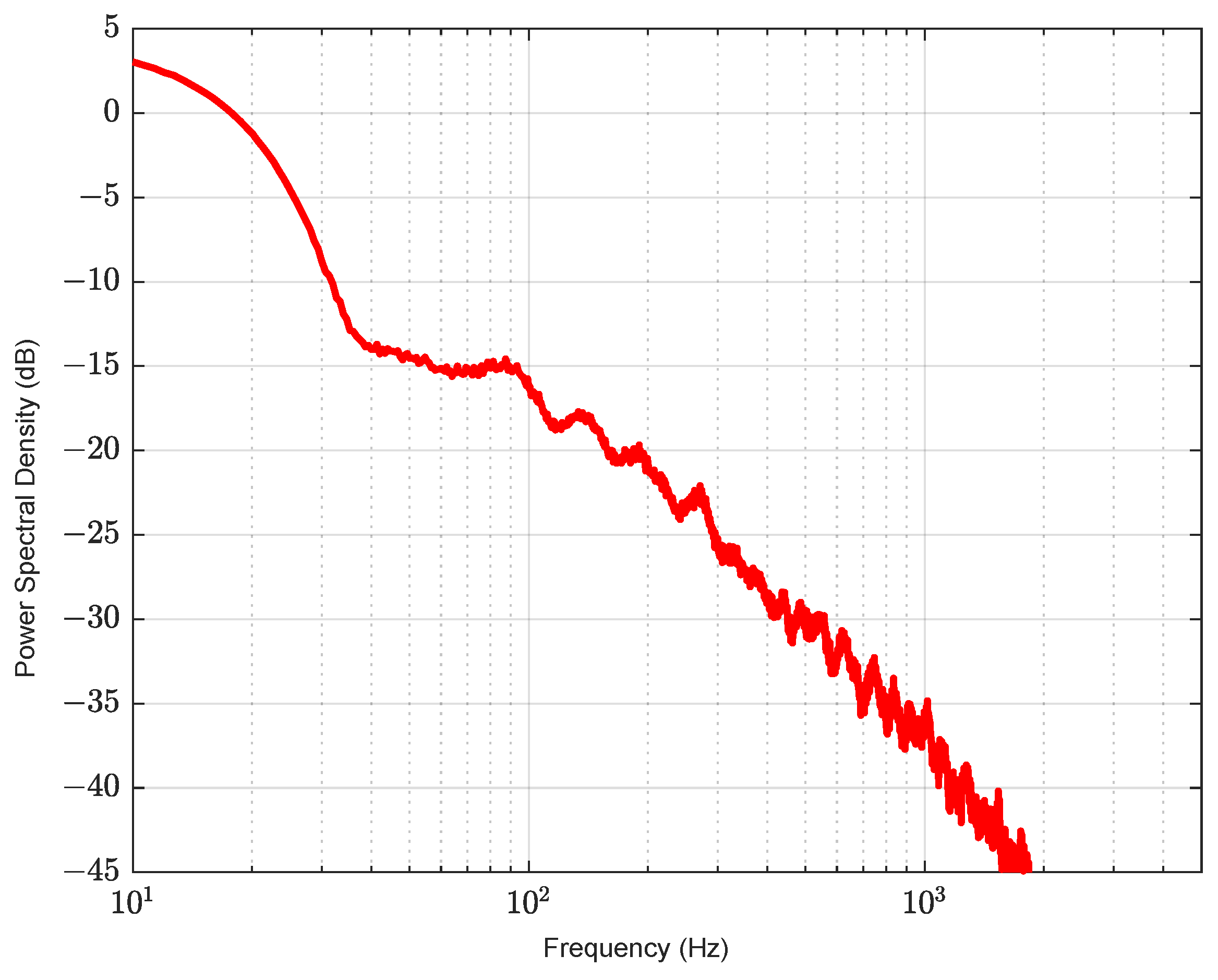
Figure 11. The green bars in the figures show the distribution of the received optical power at the output of the atmospheric turbulence simulation system, and the red lines show the distribution curve of the generated channel data. It can be seen that the distributions of the received optical power and the generated channel data were in good agreement. The figures show that the system can effectively simulate different turbulence channels based on different parameters. The power spectral density of received signal is also given in
Figure 12,
Figure 13 and
Figure 14. It can be seen that the bandwidth of the received optical power was approximately 2 kHz.
5.3. Experimental Results of the Data Obtained from the Field Experiment
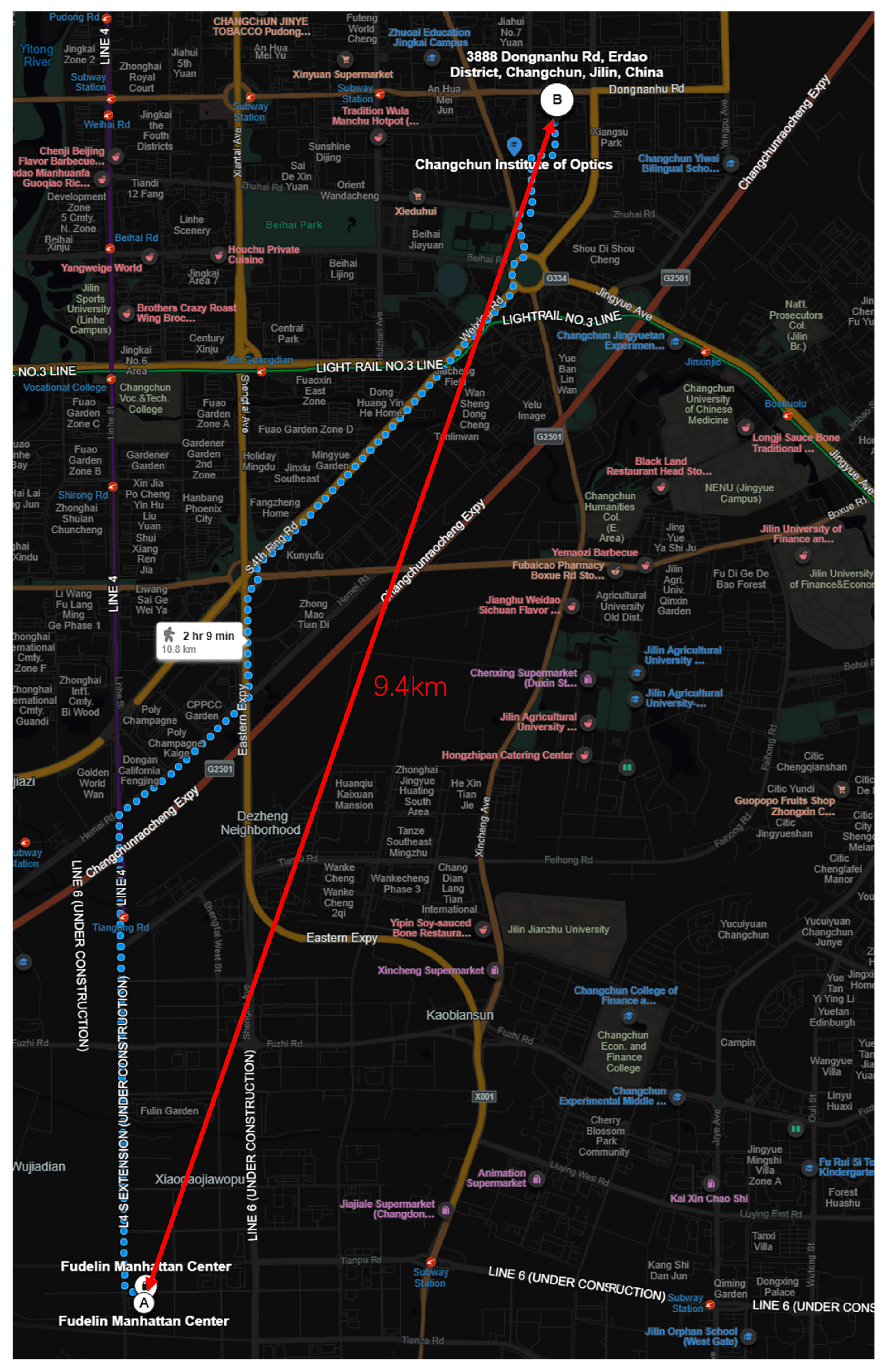
To obtain some atmospheric turbulence channel data and verify the simulation effect of the system on the real channels, an FSO field experiment with a distance of 9.4 km was carried out in Changchun.
Figure 15 shows the laser link used in the experiment. Point A marked in the figure is close to the Fudelin Manhattan Center in Changchun City, and it was the location of the transmitter used in the experiment. Point B marked in
Figure 15 was the location of the receiver used in the experiment, which is close to the Changchun Institute of Optics, Fine Mechanics and Physics, Chinese Academy of Sciences. A Teraxion narrow linewidth laser with a linewidth less than 5 kHz was used as the light source at the transmitter. The transmitting power was set at 35 dBm by an Erbium-doped fiber amplifier, and the sample rate at the receiver was set at 20 kHz. Meanwhile, the diameter of the transmitting lens was set at 2 cm, and the diameter of the receiving lens was set at 8 cm.
Analyzing the experimental results, it can be obtained that the atmospheric structure constant
Cn2 was 1.32 × 10
−16 m
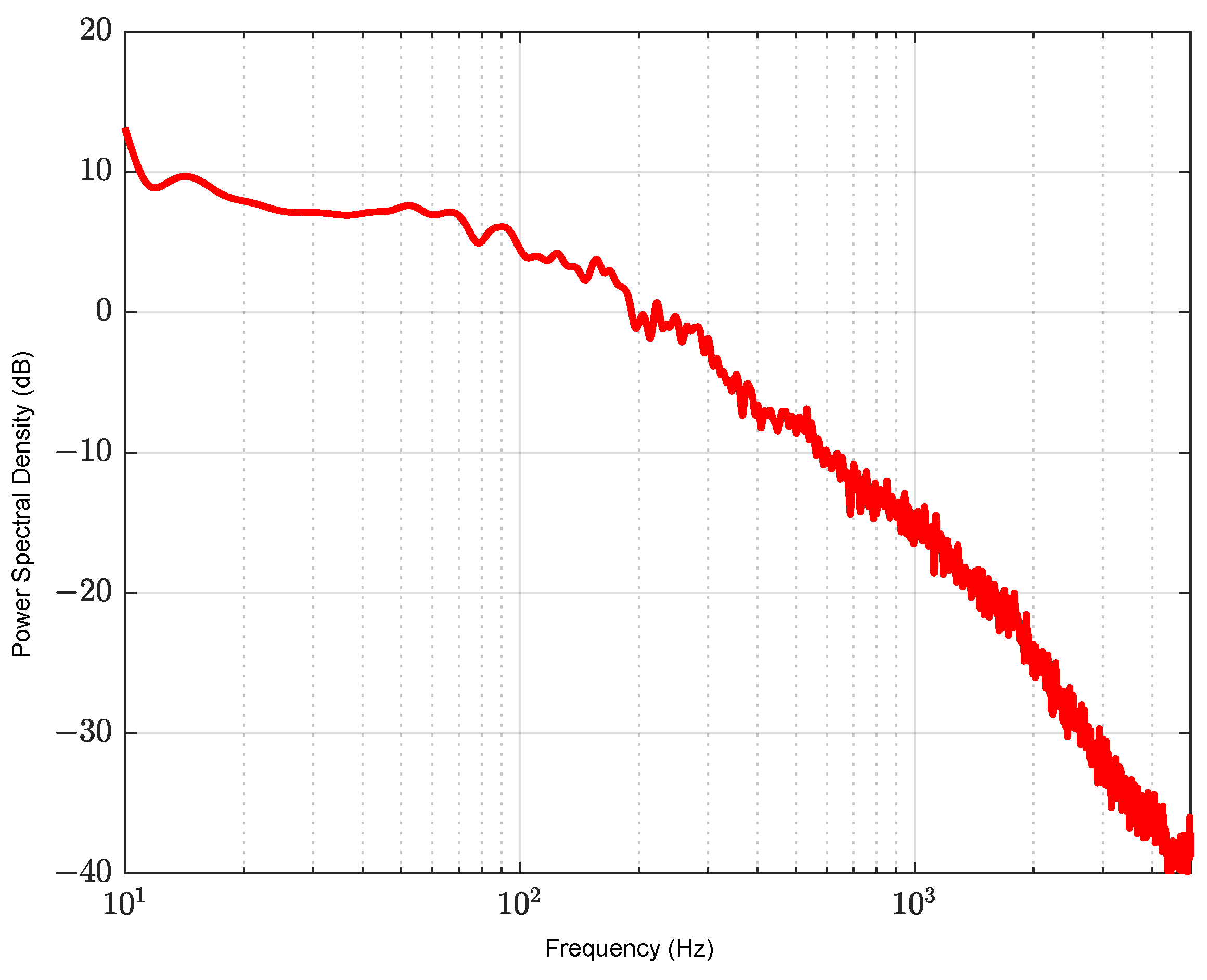
−2/3. This indicates that the turbulence was weak during the field experiment. The power spectral density of the received signal in the field experiment is shown in
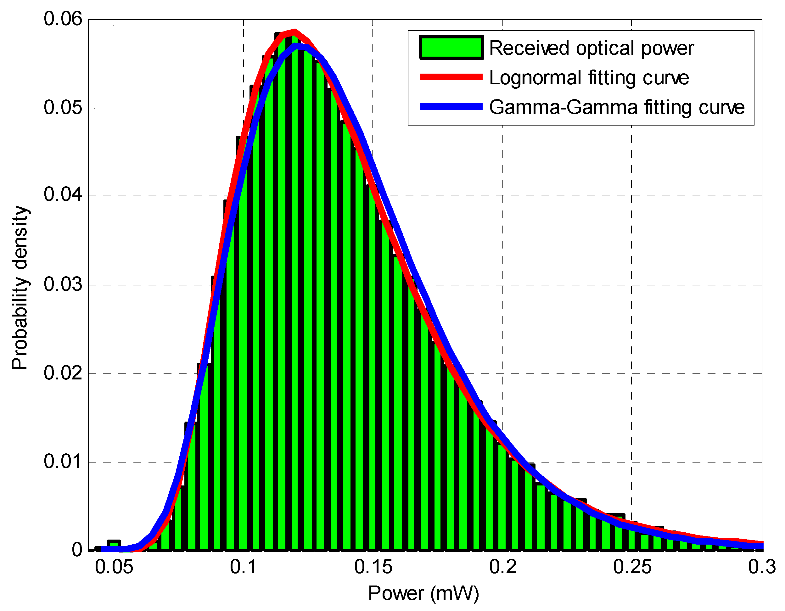
Figure 16. It can be seen that the optical power received in the experiment contained very few frequency components above 5 kHz. In
Figure 17, the distribution of the received optical power, the lognormal fitting curve at
σR2 = 0.16, and the Gamma–Gamma fitting curve at
and
are plotted. The results indicate that the optical power received by the receiver was mainly concentrated at about 0.12 mW, and the lognormal distribution was more accurate in modeling the experimental results.
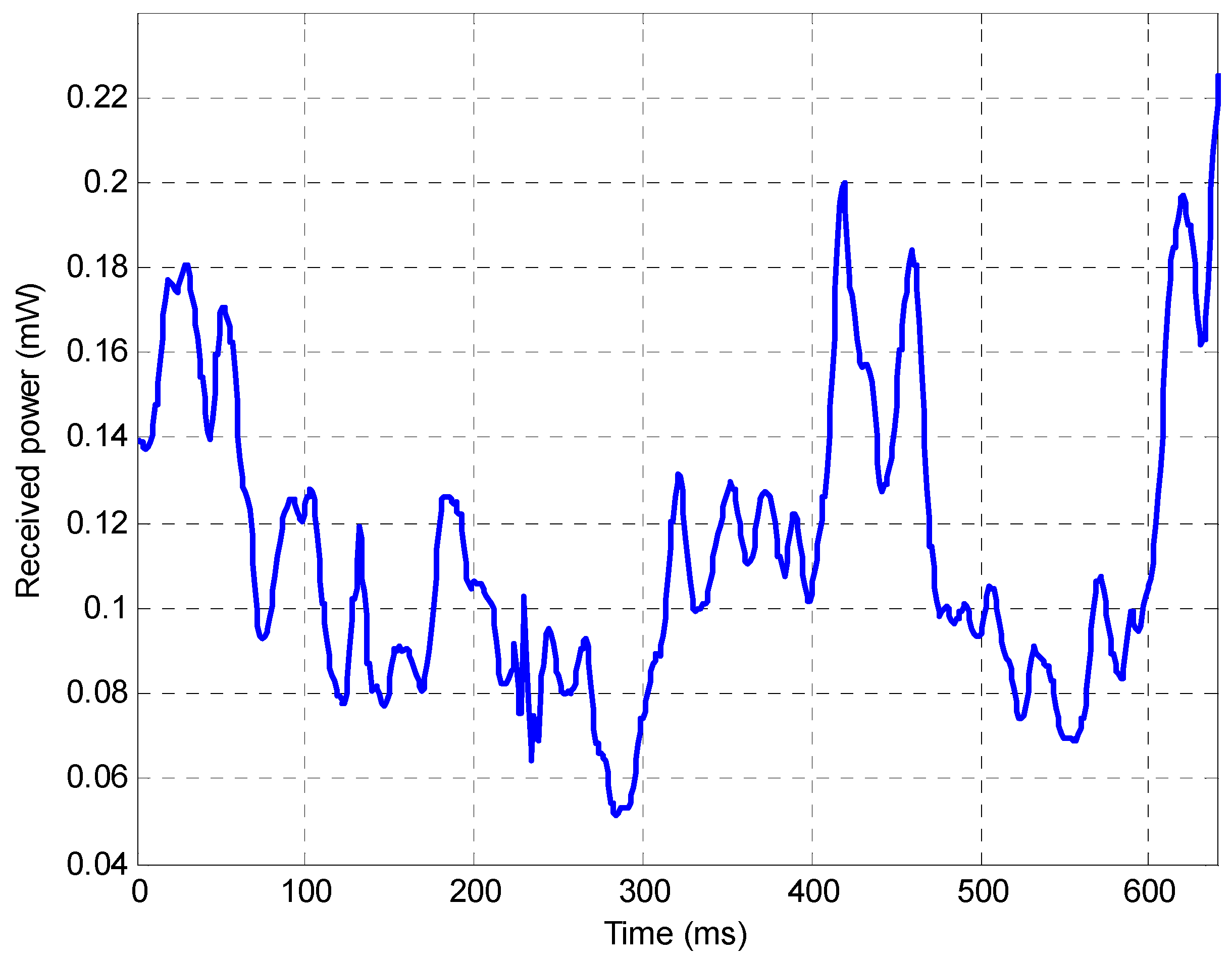
Then, the atmospheric turbulence channel data obtained from the field experiment were sent to the atmospheric turbulence simulation system. In
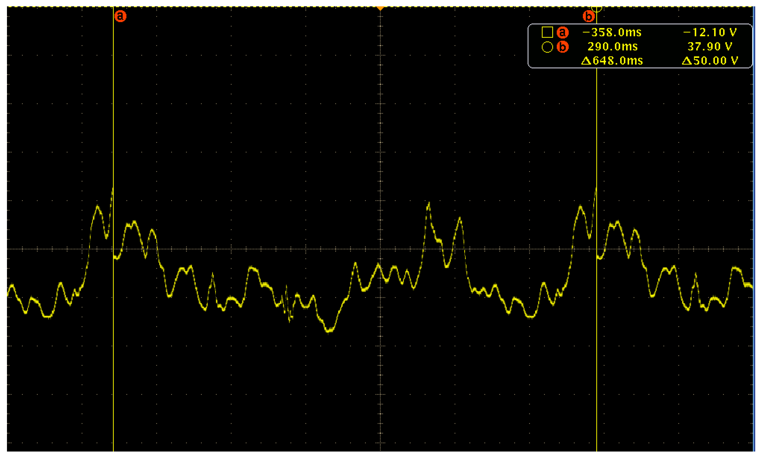
Figure 18, part of the received optical power obtained from the field experiment is plotted. The waveform of the output signal of the optical power meter displayed by the oscilloscope is given in
Figure 19.
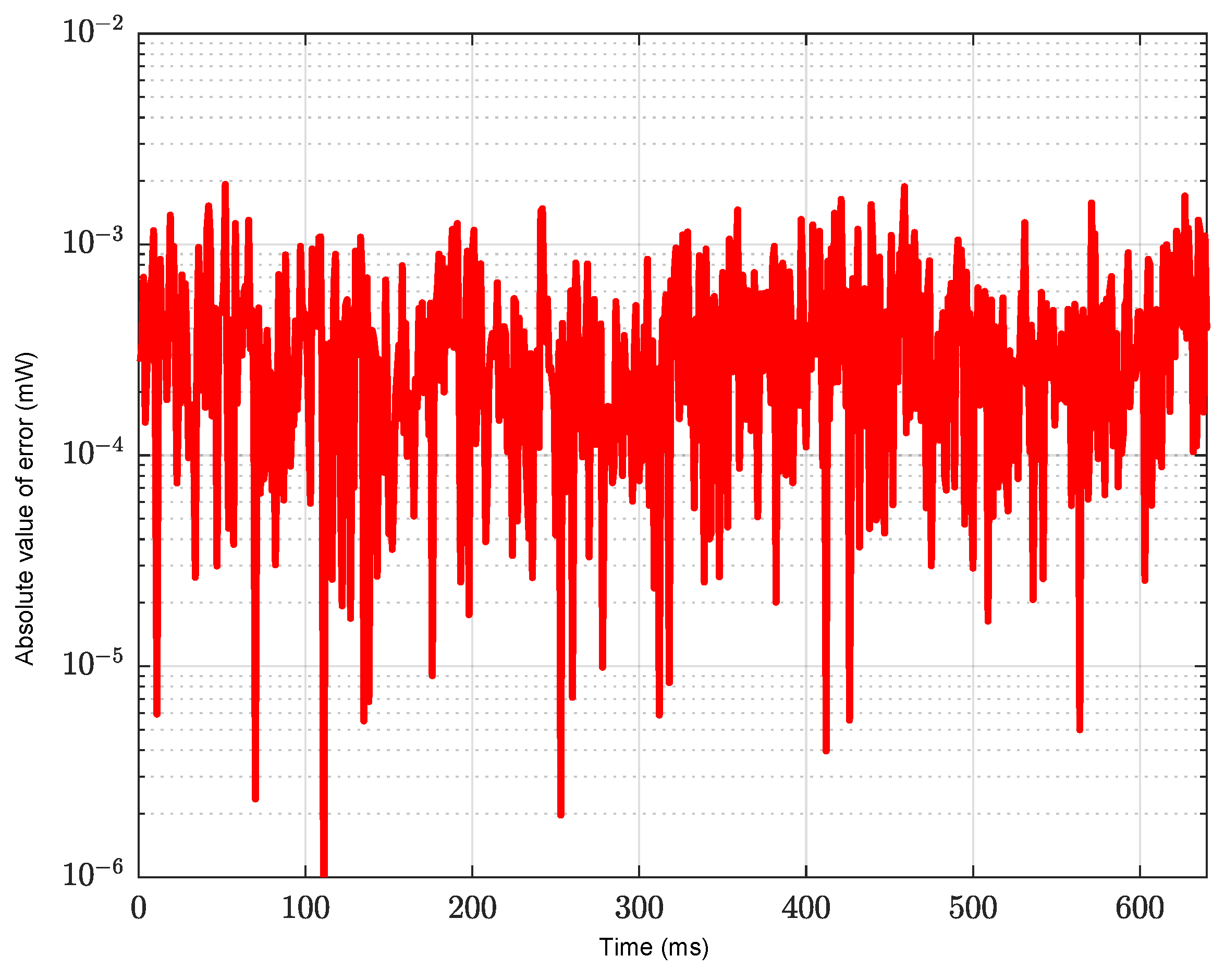
Figure 20 shows the absolute value of the error between the result of the field experiment and the result reproduced by the system. From these figures, it can be seen that there was a high degree of agreement between the two results, which shows that the system can effectively simulate the influence of the actual atmospheric channel on the FSO system.
6. Discussion
We introduced an atmospheric turbulence simulation system for an FSO system based on the use of a VOA. The system has a dynamic execution range of 30 dB and an execution rate of 1 MHz, while also having an execution accuracy of over 0.1 dB. Compared with the atmospheric turbulence simulation pool [
14], the atmospheric turbulence simulation system can accurately reproduce specific atmospheric channels. The execution rate of the system is also higher than that of the simulators using the phase screen generation method [
15] or a liquid crystal spatial light modulator (the execution rate of these simulators is only a few hundred Hz) [
16,
17,
18]. Compared with the atmospheric turbulence simulator in [
19], consisting of two point sources, a commercially available deformable mirror, and two random phase plates, the structure of the proposed system is simpler. The experimental results shown in
Figure 17 indicate that the average error between the results of the field experiment and the results generated by the simulation system is less than 10
−2 mW, which proves the superiority of the system.
Furthermore, the system can also be potentially applied to channel model processing in the field of quantum communication, which will greatly facilitate the testing of quantum communication systems similar to those mentioned in [
24,
25,
26].
However, like any other system, the proposed system has its limitations. The dynamic execution range of the system may not be sufficient to simulate atmospheric channels under extreme fading conditions. Meanwhile, the system is unable to simulate the phase fluctuations caused by atmospheric turbulence. These limitations will be gradually improved in future research.
7. Conclusions
In this paper, the atmospheric turbulence simulation system for an FSO system was proposed. The design of the system and the measurement and recording methods of atmospheric turbulence channels were introduced. Then, the experiments were described. The results showed that the proposed system can effectively simulate the influence of atmospheric turbulence channels on FSO systems, and its appearance makes it possible to simulate repeatable atmospheric channels indoors.
Author Contributions
Methodology, L.L.; software, N.J.; validation, L.L., N.J. and Z.W.; investigation, J.W.; writing—original draft preparation, L.L.; writing—review and editing, Z.W. and J.W. All authors have read and agreed to the published version of the manuscript.
Funding
This work was supported by the Project: Scientific Research Equipment of Chinese Academy of Sciences.
Institutional Review Board Statement
Not applicable.
Informed Consent Statement
Not applicable.
Data Availability Statement
Data underlying the results presented in this paper are not publicly available at this time but may be obtained from the authors upon reasonable request.
Acknowledgments
The authors gratefully acknowledge the Optical Communication Laboratory of CIOMP for the use of their equipment. The authors wish to thank the anonymous reviewers for their valuable suggestions.
Conflicts of Interest
The authors declare no conflicts of interest.
References
- Chen, J.; Huang, Y.; Cai, R.; Zheng, A.; Yu, Z.; Wang, T.; Gao, S. Free-Space Communication Turbulence Compensation by Optical Phase Conjugation. IEEE Photonics J. 2020, 12, 7905611. [Google Scholar] [CrossRef]
- Li, K.; Ma, J.; Tan, L.; Yu, S.; Zhai, C. Performance Analysis of Fiber-based Free-space Optical Communications with Coherent Detection Spatial Diversity. Appl. Opt. 2016, 55, 4649–4656. [Google Scholar] [CrossRef] [PubMed]
- Wang, Y.; Wang, Y.; Lu, W. Secrecy Performance Analysis of Mixed RF/FSO Systems Based on RIS Reflection Interference Eavesdropper. Photonics 2023, 10, 1193. [Google Scholar] [CrossRef]
- Singya, P.K.; Kumar, N.; Bhatia, V.; Alouini, M.S. On the Performance Analysis of Higher Order QAM Schemes over Mixed RF/FSO Systems. IEEE Trans. Veh. Technol. 2020, 69, 7366–7378. [Google Scholar] [CrossRef]
- Wang, Z.; Zhong, W.D.; Fu, S.; Lin, C. Performance Comparison of Different Modulation Formats over Free-space Optical (FSO) Turbulence Links with Space Diversity Reception Technique. IEEE Photonics J. 2009, 1, 277–285. [Google Scholar] [CrossRef]
- Varotsos, G.K.; Aidinis, K.; Nistazakis, H.E.; Gajic, Z. Energy-Efficient Emerging Optical Wireless Links. Energies 2023, 16, 6485. [Google Scholar] [CrossRef]
- Lv, P.-F.; Hong, Y.-Q. Self-Pilot Tone Based Adaptive Threshold RZ-OOK Decision for Free-Space Optical Communications. Photonics 2023, 10, 714. [Google Scholar] [CrossRef]
- Moradi, H.; Falahpour, M.; Refai, H.H.; LoPresti, P.G.; Atiquzzaman, M. BER Analysis of Optical Wireless Signals through Lognormal Fading Channels with Perfect CSI. In Proceedings of the 2010 17th International Conference on Telecommunications, Doha, Qatar, 4–7 April 2010. [Google Scholar]
- Kumar, N.; Khandelwal, V. Simulation of MIMO-FSO System with Gamma-Gamma Fading under Different Atmospheric Turbulence Conditions. In Proceedings of the 2019 International Conference on Signal Processing and Communication (ICSC), Noida, India, 7–9 March 2019. [Google Scholar]
- Chang, Y.; Liu, Z.; Yao, H.; Gao, S.; Dong, K.; Liu, S. Performance Analysis of Multi-Hop FSOC over Gamma-Gamma Turbulence and Random Fog with Generalized Pointing Errors. Photonics 2023, 10, 1240. [Google Scholar] [CrossRef]
- Wu, Y.; Li, G.; Kong, D. Performance Analysis of Relay-Aided Hybrid FSO/RF Cooperation Communication System over the Generalized Turbulence Channels with Pointing Errors and Nakagami-m Fading Channels. Sensors 2023, 23, 6191. [Google Scholar] [CrossRef] [PubMed]
- Palliyembil, V.; Jagadeesh, V.K.; Muthuchidamdaranathan, P. Analysis of Free Space Optical DPSK-SIM Based Communication System over Málaga Distributed Channel with Misalignment Fading. In Proceedings of the 2019 TEQIP III Sponsored International Conference on Microwave Integrated Circuits, Photonics and Wireless Networks (IMICPW), Tiruchirappalli, India, 22–24 May 2019. [Google Scholar]
- Mishra, N.; Kumar, D.S. Outage Analysis of Relay Assisted FSO Systems over K-distribution Turbulence Channel. In Proceedings of the 2016 International Conference on Electrical, Electronics, and Optimization Techniques (ICEEOT), Chennai, India, 3–5 March 2016. [Google Scholar]
- Ghassemlooy, Z.; Minh, H.L.; Rajbhandari, S.; Perez, J.; Ijaz, M. Performance Analysis of Ethernet/Fast-Ethernet Free Space Optical Communications in a Controlled Weak Turbulence Condition. J. Light. Technol. 2012, 30, 2188–2194. [Google Scholar] [CrossRef]
- Salmanowitz, J.; Zandt, N.R.V. Phase Screen Generation Methods for Simulating Light Propagation through Non-Kolmogorov Turbulence. In Proceedings of the 2022 IEEE Aerospace Conference (AERO), Big Sky, MT, USA, 5–12 March 2022. [Google Scholar]
- Liu, Z.; Zheng, C.; Lin, P.; Wang, T. Atmospheric Turbulence Simulation Experiment Based on Liquid Crystal Spatial Light Modulator. In Proceedings of the 2021 13th International Conference on Advanced Infocomm Technology (ICAIT), Yanji, China, 15–18 October 2021. [Google Scholar]
- Wilcox, C.C.; Andrews, J.R.; Restaino, S.R.; Martinez, T.; Teare, S.W. Atmospheric Turbulence Generator Using a Liquid Crystal Spatial Light Modulator. In Proceedings of the 2007 IEEE Aerospace Conference (AERO), Big Sky, MT, USA, 3–10 March 2007. [Google Scholar]
- Burger, L.; Litvin, I.; Forbes, A. Simulating atmospheric turbulence using a phase-only spatial light modulator. S. Afr. J. Sci. 2008, 104, 129–134. [Google Scholar]
- Lee, J.H.; Shin, S.; Park, G.N.; Rhee, H.; Yang, H. Atmospheric Turbulence Simulator for Adaptive Optics Evaluation on an Optical Test Bench. Curr. Opt. Photonics 2017, 1, 107–112. [Google Scholar] [CrossRef]
- Andrews, L.C.; Phillips, R.L.; Hopen, C.Y. Laser Beam Scintillation with Applications, 1st ed.; SPIE Press: Bellingham, WA, USA, 2001; pp. 67–68. [Google Scholar]
- Fidler, F. Optical Communications from High Altitude Platforms. Ph.D. Thesis, Institute of Communications and Radio Frequency Engineering, Vienna University of Technology, Vienna, Austria, 2007. [Google Scholar]
- Uysal, M.; Capsoni, C.; Ghassemlooy, Z.; Boucouvalas, A.; Udvary, E. Optical Wireless Communications: An Emerging Technology, 1st ed.; Springer: Cham, Switzerland, 2016; pp. 25–26. [Google Scholar]
- Andrews, L.C.; Phillips, R.L. Laser Beam Propagation Through Random Media, 2nd ed.; SPIE Press: Bellingham, WA, USA, 2005; pp. 409–410. [Google Scholar]
- Zhou, L.; Lin, J.; Xie, Y.; Lu, Y.; Jing, Y.; Yin, H.; Yuan, Z. Experimental Quantum Communication Overcomes the Rate-Loss Limit without Global Phase Tracking. Phys. Rev. Lett. 2023, 130, 250801. [Google Scholar] [CrossRef]
- Cao, Y.; Li, Y.; Yang, K.; Jiang, Y.; Li, S.; Hu, X.; Abulizi, M.; Li, C.-L.; Zhang, W.; Sun, Q.-C.; et al. Long-distance free-space measurement-device-independent quantum key distribution. Phys. Rev. Lett. 2020, 125, 260503. [Google Scholar] [CrossRef] [PubMed]
- Cao, X.Y.; Li, B.H.; Wang, Y.; Fu, Y.; Yin, H.L.; Chen, Z.B. Experimental quantum e-commerce. Sci. Adv. 2024, 10, eadk3258. [Google Scholar] [CrossRef]
| Disclaimer/Publisher’s Note: The statements, opinions and data contained in all publications are solely those of the individual author(s) and contributor(s) and not of MDPI and/or the editor(s). MDPI and/or the editor(s) disclaim responsibility for any injury to people or property resulting from any ideas, methods, instructions or products referred to in the content. |
© 2024 by the authors. Licensee MDPI, Basel, Switzerland. This article is an open access article distributed under the terms and conditions of the Creative Commons Attribution (CC BY) license (https://creativecommons.org/licenses/by/4.0/).


