Abstract
In order to study the transmission characteristics of Airy beams in the plasma sheath, the flow field around a hypersonic vehicle was numerically simulated and analyzed based on the Navier–Stokes (N-S) equation and a turbulence model. Then, according to the characteristics of the thickness of the plasma flow field around the supersonic vehicle at the centimeter level, the double fast Fourier transform (D-FFT) algorithm and multi-random phase screens theory were used to predict the propagation characteristics of the Airy beams in the turbulent plasma sheath. The results show that the lower the height and the higher the speed, the smaller the thickness of the plasma sheath shock layer. The refractive index variation in the sheath shock layer has a significant influence on Airy beam transmission. At the same time, the transmission distance and the attenuation factor of the Airy beams also change the transmission quality of the Airy beams. The larger the attenuation factor, the smaller the drift, and the standard deviation decreases with an increase in the refractive index. Airy beams have smaller drifts compared to Gaussian beams and have advantages in suppressing turbulence.
1. Introduction
In recent years, Airy beams have attracted extensive attention for their unique properties, such as non-diffraction, lateral self-acceleration, and self-healing [1,2,3,4,5]. Its own generation method [6], trajectory control method [7], plasma channel [8], and other fields [9,10] have been the focus of research. In view of the advantages of Airy beams, Tao et al. derived the expression of Airy beam propagation in the atmosphere and discussed the effect of atmospheric turbulence intensity on beam propagation [11]. Wen et al. deduced the propagation coefficient of Airy beams in turbulent oceans based on diffraction theory [12]. However, in addition to turbulence in the atmosphere [13,14] and oceans [15], turbulence also exists in the plasma sheath around supersonic flight targets [16,17].
When the aircraft is flying in the atmosphere at hypersonic speed, the surrounding air is rapidly dissociated and ionized, forming a plasma-covered flow field [18,19,20,21,22,23]. The plasma will attenuate the electromagnetic wave and even interrupt the signal [24,25]. Studies show that the plasma sheath is unstable, so turbulence is also one of the key factors affecting the “black barrier effect”. Some researchers have also used the strong penetration properties of terahertz waves to weaken the “black barrier” problem of the plasma sheath [26,27]. Subsequently, a few scholars have studied the transmission characteristics of high-frequency beams in the plasma sheath. For example, Zang et al. discussed the phase characteristics of the plasma laser signal and the information transmission characteristics in the shock tube [28], providing an important reference. In addition, only a few scholars have studied the transmission characteristics of Gaussian beams in turbulent plasma sheaths, and it was initially found that visible and near-infrared bands are more suitable [29,30]. However, there have been no published reports on Airy beams in plasma turbulence.
It is worth noting that a single fast Fourier transform (S-FFT) algorithm can be used for the long-distance transmission of atmospheric [31,32] and ocean [33,34] turbulence, while for short-distance transmission at the centimeter and millimeter levels inside the plasma sheath, the S-FFT algorithm will reduce sampling problems and eventually lead to signal distortion. Therefore, we compared three Fresnel diffraction integration algorithms and chose to use the D-FFT algorithm of Fresnel diffraction integration to study the beam transmission process between two phase screens.
The rest of this article is arranged as follows. Section 2 mainly describes the simulation principle of the flow field in the plasma sheath, compares three Fresnel diffraction integration algorithms, and also describes the theory of simulating beam propagation using multi-random phase screens. The main results and a discussion of them are given in Section 3. The results are helpful for understanding the internal characteristics of a plasma sheath, improving communication quality and solving the black barrier effect.
2. Statistical Analysis of the Turbulent Flow Field around a Hypersonic Vehicle
2.1. Airy Beams
The expression of Airy beams in free space in a rectangular coordinate system is as follows [35]:
where is the Wave number, and is the Airy function.
where is the attenuation factor, which can constrain the energy of the Airy beams to become a finite energy Airy beam. When the attenuation factor is 0, resulting in infinite energy Airy beams. and are the axial scales.
2.2. Modeling of Plasma Sheath
The N-S equation with the appropriate closure models and turbulence model is used. In the Cartesian coordinate system, the two-temperature thermomechanical model proposed in 1989 and the seven-component air chemical reaction model are considered [36]. The turbulent flow field around a hypersonic aircraft is given as follows [37,38,39]:
where and are the conserved variable vector and the source term vector, respectively. Taking direction as an example, and are the inviscid flux vector and the viscous flux vector, respectively. , and have the same form; and are thermal conductivity and turbulent thermal conductivity, respectively. , , and are the instantaneous velocity components in three directions, respectively. is the turbulent kinetic energy, is the vibration source term, and is the mass fraction of each component. is the shear stress tensor component that can be closed by the turbulence model [40]., , and are the vibration energy, sensible enthalpy, and density of each component, respectively, and the subscripts represent the species . , and are the density, pressure, and average velocity of the mixture, respectively. , and are the internal energy, the turbulent internal energy, and the internal temperature of the mixture, respectively. Based on the finite volume method, the advection upstream splitting method can solve the N-S equation via the pressure-based weight function (AUSMPW+) [41]. The implicit lower–upper symmetric Gauss–Seidel relaxation method (LU-SGS) is used for the time-marching algorithm [42].
In our simulation process, in order to accurately solve the N-S equation, we selected compressible flow and used a gas component model. A two-temperature thermodynamic equilibrium model and the seven-component Gupta chemical reaction model were used. For the boundary problem, the parameters of temperature and pressure were calculated according to the flow velocity and height, the wall was the isothermal wall, and the exit state was extrapolated. The result was observed according to the degree of convergence.
2.3. Statistical Analysis of Flow Field Data
The Gladstone–Dale law is used to obtain index-of-refraction variation, which is proportional to the local density [43,44,45,46]:
where is the wavelength, is the local electron density, and is the Gladstone–Dale constant, which is defined as follows [29,43]:
As shown in Figure 1, if Airy beams are propagated in a positive direction along the X-axis, the head of the vehicle will change significantly due to the compression of velocity. The wall is the reference point (that is, the origin of the rectangular coordinate system). The value range of head region 1 is x = [−25 cm, −15 cm], y = [−83.82 cm, −92.55 cm], and z = [16.60 cm, 26.00 cm]; the value range of head region 2 is x = [−15 cm, 0 cm], y = [−102.82 cm, −92.55 cm], and z = [36.00 cm, 26.00 cm]; and the value range of head region 3 is x = [−15 cm, 0 cm], y = [−45.55 cm, −35.86 cm], and z = [50.60 cm, 60.00 cm] (shock layer on the left side of the wall). It is divided into 10 equal parts along the x-direction, and a spherical model is established with the typical correlation length in supersonic turbulence as the radius (which is the thickness of the plasma sheath). All the data on the sphere are analyzed statistically, and the refractive index variance of each grid point is calculated. In addition, the boundary values of the flow field are solved by using an extrapolation method.
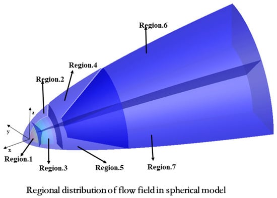
Figure 1.
Distribution of different regions of the model. Region (1–3): head region distribution; region (4–7): side regional distribution.
2.4. Simulation of Multiple Random Phase Screens in the Turbulent Plasma Sheath
2.4.1. The Fresnel Diffraction Integral and the S-FFT, T-FFT, and D-FFT Algorithms
The S-FFT, T-FFT, and D-FFT algorithms are all based on the Fresnel diffraction formula, but the requirements for diffraction distance and sampling points differ. The three algorithms are introduced and compared below [47]:
In the case of paraxial approximation, the Fresnel diffraction integral can be expressed as:
where and are the complex amplitudes of the light field at points on the diffraction plane and the observation plane, is the wavelength, and is the distance from the observation plane to the diffraction screen. Therefore, the fast and accurate completion of the integration of Equation (10) can solve the problem of giving the complex amplitude of the light wave on the observation surface in the subsequent medium space from the light wave complex amplitude distribution in the source plane. The S-FFT algorithm for the Fresnel diffraction integral can also be simplified as:
where “FFT {}” represents the completion of the fast Fourier transform. Because this algorithm requires only a single Fourier transform, it is called the S-FFT algorithm.
The T-FFT algorithm for the Fresnel diffraction integral can also be simplified as:
where “FFT-1{}” represents the completion of the fast inverse Fourier transform.
The D-FFT algorithm for the Fresnel diffraction integral can also be simplified as:
Assuming that the wavelength of the beam remains unchanged, the diffraction distance and the sampling point are changed, and the ability of the S-FFT algorithm, the T-FFT algorithm, and the D-FFT algorithm to suppress the sampling point is compared. In the simulation, the beam wavelength is 1064 nm, the simulated side length is 8 mm, the central square light transmission hole is 4 mm, and the diffraction screen size is L0 = 7 mm. The simulation results for different diffraction distances and sampling points are as follows:
In Figure 2, the (a) represents the S-FFT algorithm, the (b) represents the D-FFT algorithm, and the (c) represents the T-FFT algorithm. The d represents the distance between two adjacent phase screens, and N represents the sampling points on each phase screen. As shown in Figure 2, the distance of the (a) is greater than that of the (b) and (c), and the sampling point of the (b) is smaller than that of the (c). It can be seen that the S-FFT and the T-FFT algorithms have requirements for transmission distance and sampling points, and it is also shown that the D-FFT algorithm has apparent advantages in dealing with short-distance diffraction integration problems. Therefore, the D-FFT algorithm is the most suitable for the short-distance transmission problem when a multi-random phase screen is used.
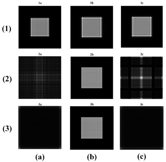
Figure 2.
Comparison of three calculation points at different transmission distances and sampling points. (1a–1c) d = 0.1 m, N = 512; (2a–2c) d = 0.02 m, N = 512; (3a–3c) d = 0.02 m, N = 1024.
2.4.2. Multi-Random Phase Screens Theory
The D-FFT algorithm based on the Fresnel diffraction integral is used to solve the transmission of Airy beams between two adjacent screens. Then, multi-random phase screens generated by the power spectrum inversion method are used to simulate the influence of plasma sheath turbulence. A schematic diagram of the multi-random phase screen is shown in Figure 3.
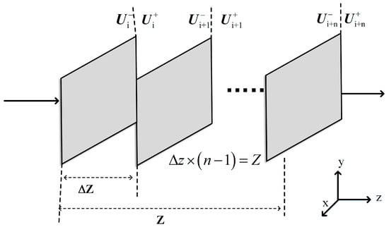
Figure 3.
Schematic diagram of the multi-random phase screen.
Then, the turbulent random phase screen of the plasma sheath is generated by the spectral inversion. Firstly, a complex random matrix of order with mean 1 and variance 0 needs to be generated in the frequency domain, which is filtered by the turbulence power spectrum of the plasma sheath, and then the random phase screen of the plasma sheath turbulence can be obtained by the inverse Fourier transform. The turbulent power spectrum of the plasma sheath is [44,48]:
where is the refractive index variance, is the turbulent outer scale, and and are frequencies in different directions.
The phase spectrum can be obtained from the refractive index spectrum:
The variance of the phase spectrum is:
where is the spacing of any two random phase screens, is the number of samples, and is the grid spacing.
The random phase screen in the spatial space can be obtained using the Fourier transform:
Superimpose this perturbation on to obtain the expression at the transmission distance:
Finally, the same algorithm is used to calculate the distance after the second transmission. Accordingly, the light intensity at the transmission distance can be obtained. Therefore, the D-FFT algorithm based on the Fresnel diffraction integral is used to solve the transmission of Airy beams between two adjacent screens. Then, multi-random phase screens generated by the power spectrum inversion method are used to simulate the influence of plasma sheath turbulence.
3. Transmission of Airy Beams in the Turbulent Plasma Sheath
3.1. Analysis of Time-Varying Parameters in the Turbulent Plasma Sheath Flow Field
In order to analyze the influence of different flight conditions on the parameters of the flow field around the hypersonic ball model, the flow field parameters at different flight Mach numbers and flight altitudes were numerically calculated. In the simulation process, in order to accurately solve the N-S equation, we selected compressible flow. In the selected gas model, the free-flowing air is assumed to consist of 79% N2 and 21% O2. The two-temperature thermodynamic equilibrium model and the seven-component Gupta chemical reaction model were used. The flow field parameter distribution under different flight conditions was simulated, and the flight Mach numbers were Mach 18 and Mach 20, and the flight altitudes were 45 km and 50 km. For the boundary problem, the parameters of temperature and pressure were calculated according to the flow velocity and height; the wall was an isothermal wall, and the exit state was extrapolated. The result was observed according to the degree of convergence.
The effects of different flight conditions on the distribution of the flow field around a hypersonic vehicle are analyzed below. In the flow field of the hypersonic ball model, the parameters of the stagnation point region of the head are the most varied. The chemical non-equilibrium phenomenon is the most obvious, and the core of the study is the plasma sheath. Therefore, the following calculation results only give and analyze the flow field parameter distribution of the ball head.
Firstly, we compared the variation trends regarding temperature and pressure in the plasma sheath at different heights and speeds. As shown in Figure 4a, the translational temperature is significantly higher than the vibration temperature, and there is a significant difference with the change in the environment in the plasma sheath. It can be seen from Figure 4b that the height and speed affect the changes in pressure in the plasma sheath. Both affect the content of gas components and the chemical reaction between the gas components. The variation trend regarding the gas components in the flow field around the ball head is shown in Figure 5.
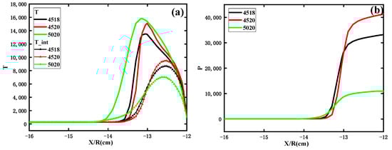
Figure 4.
Temperature and pressure in the head region under different flight conditions. (a) Temperature; (b) pressure.
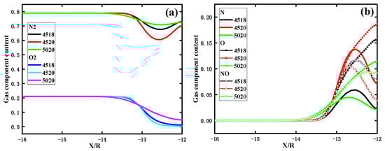
Figure 5.
The variation trends of each chemical component in the head region of the seven-component Gupta chemical reaction model. (a) The variation trends of N2 and O2 in the head region; (b) The variation trends of N, O and NO in the head region.
As shown in Figure 5, the content of nitrogen and oxygen in the head area changes dramatically. Secondly, it was found that speed is more sensitive to the effect of content than height. This is enough to show that the chemical reactions in the plasma sheath are complex and changeable. At the same time, the content of gas components also varies with the change in height and speed, which will also affect the beam’s transmission in the plasma sheath.
Figure 6 shows frequency and collision frequency schematic diagrams at different speeds and altitudes. As seen in Figure 6, the higher the speed, the lower the electron density and collision frequency inside the plasma sheath. The higher the height, the higher the electron density and collision frequency inside the plasma sheath. In other words, the larger the speed and the smaller the height, the smaller the thickness of the plasma sheath shock layer, and these differences will have a significant difference in the transmission of the beam.
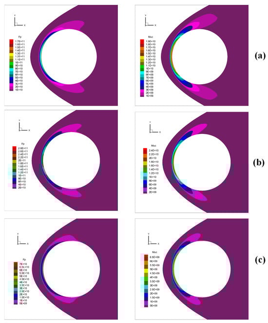
Figure 6.
Schematic diagram of frequency and collision frequency at different speeds and altitudes. (a) H = 45 Km, v = 18 Ma; (b) H = 45 Km, v = 20 Ma; (c) H = 50 Km, v = 20 Ma.
The flow field data are used when the flight altitude is 50 km, the flight speed is Mach 20, and the angle of attack is 0. The fluctuation range of the refractive index variance of the flow field near the head region is shown in Figure 7a–c. When approaching the plane wall, the refractive index changes greatly, because the turbulent state in the plasma sheath is also affected by shock waves, high temperature, high pressure, and other factors. The temperature, pressure, and fluctuations near the head are high. The changes on both sides are weaker than those in zone of the aircraft head.
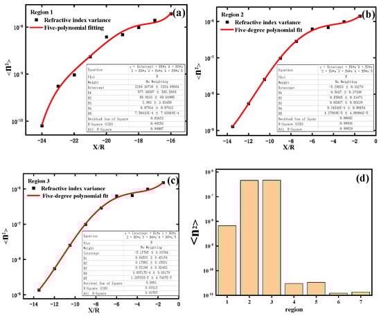
Figure 7.
The refractive index variance in the plasma sheath. (a–c) Head region; (d) All regional distribution.
In the outflow field of hypersonic vehicles, the parameters of the head stagnation area change the most. The chemical non-equilibrium phenomenon is the most obvious, and the core of the study is the plasma sheath. Therefore, the focus here is to analyze only the state of the head region. The same method gives the range of variance values of the refractive index fluctuations on both sides in Figure 7d. In the following section, the transmission characteristics of the Airy beams in the plasma sheath are analyzed in detail.
3.2. Analysis of Factors Affecting the Transmission Quality of the Airy Beams in the Turbulent Plasma Sheath
In this section, the propagation of the Airy beams in the turbulent plasma sheath is discussed, and the propagation characteristics of the Airy beams in turbulence with different fluctuation degrees are obtained. In our simulation, the transmission distance was , the phase screen size was , the number of grids was , and the phase screen spacing was (10 phase screens). The wavelength is , and the Airy beams had an attenuation factor of 0.02 and an axial scale of 0.001.
Figure 8 discusses the effect of the refractive index variance in the Airy beams. The distribution of light intensity and phase under different refractive index variances was analyzed when 20 cm Airy beams were transmitted. The refractive index variances were 10−10, 10−8, and 10−6, respectively. As can be seen from Figure 8, with an increase in the refractive index variance, the dispersion degree of the light spot is enhanced, and the phase fluctuation gradually increases. Figure 9 discusses the transmission characteristics of Airy beams propagating over different distances. The selected distances were 5 cm, 10 cm, and 20 cm, respectively. In addition, 10 phase screens were used, so the distance between two adjacent phase screens was very small. They were 0.005 m, 0.01 m, and 0.02 m, respectively. As can be seen from Figure 9, the longer the propagation distance, the higher the dispersion degree of the light spot, and the greater the phase fluctuation. Therefore, for short-distance transmission in a plasma sheath communication system, the turbulent effect cannot be ignored.
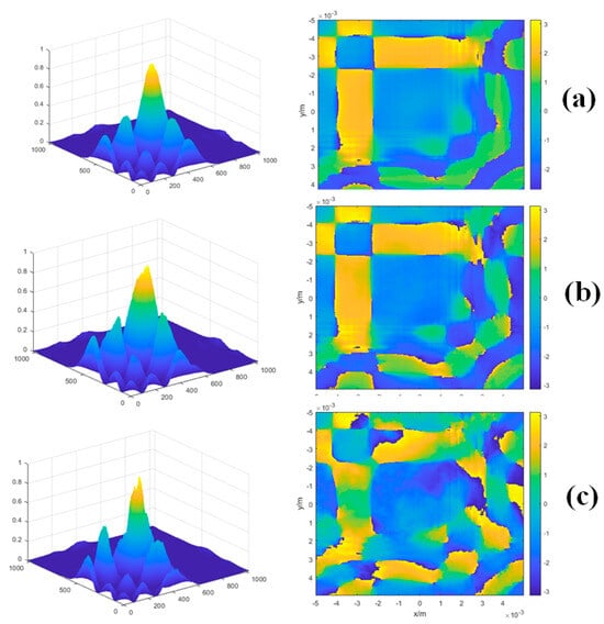
Figure 8.
Transmission characteristics of the Airy beams under different refractive index variances. (a) ; (b) ; (c) .
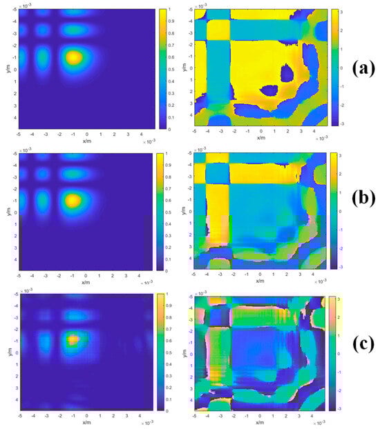
Figure 9.
Transmission characteristics of the Airy beams under different distances. (a) x = 5 cm; (b) x = 10 cm; (c) x = 20 cm.
Figure 10 discusses the distribution of Airy beam intensity and phase for different attenuation factors. As the attenuation factor increases, the light intensity gradually converges to the center, and the disturbance shows signs of decreasing. The attenuation factor has a lower disturbing effect on the Airy beam phase than on the Airy beam light intensity.
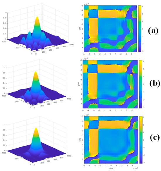
Figure 10.
Propagation characteristics of Airy beams with different attenuation factors. (a) a = 0.02; (b) a = 0.1; (c) a = 0.3.
Figure 11 analyzes the drift characteristics of Airy beams. Figure 11a discusses the drift characteristics of Airy beams under different attenuation factors. The values of the attenuation factors are 0.02, 0.1, and 0.3, respectively, and the standard deviations of the curves under the attenuation factors are and , respectively. In addition, comparing Gaussian beams with Airy beams, Figure 11b shows that Airy beams have a better ability to suppress turbulence than Gaussian beams.
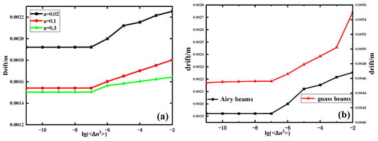
Figure 11.
Analysis of Airy beam drift characteristics. (a) The drift characteristics of Airy beams under different attenuation factors; (b) The comparison of Airy beams and Gaussian beams.
4. Conclusions and Perspectives
In this study, the turbulent flow field in the plasma sheath was numerically simulated based on the three-dimensional N-S equation and a turbulent two-equation model. The D-FFT algorithm based on the Fresnel diffraction integral was used to study the transmission characteristics of Airy beams in the plasma sheath. The results show that the lower the height and the higher the speed, the smaller the thickness of the plasma sheath shock layer, which will also affect the distribution of the internal frequency and collision frequency of the plasma sheath. The plasma sheath communication system has a critical value of refractive index variance. Above the critical point, the refractive index has a significant effect on the beam transmission quality. Refractive index variance, transmission distance, and attenuation factor are all important factors affecting the transmission quality of Airy beams. The larger the refractive index variance and transmission distance, the worse the Airy beam transmission quality, and the worse the serious phase disturbance. The larger the Airy beam attenuation factor, the smaller the beam drift, and the less the obvious phase disturbance, indicating a stronger ability to suppress turbulence. Airy beams have a smaller drift index than Gaussian beams. It can be seen that Airy beams have a better anti-jamming ability than Gaussian beams when applied to atmospheric communication as an information carrier.
The research in this paper will help us to understand the internal characteristics of the plasma sheath and improve communication quality. At the same time, it provides a theoretical basis for more complex models and beams and also provides a theoretical basis for experiments.
Author Contributions
X.G.: conceptualization, methodology, software, investigation, data curation, writing—original draft preparation. Y.H.: validation, writing—review and editing, funding acquisition. J.W.: supervision, formal analysis, resources. S.X.: visualization, project administration. All authors have read and agreed to the published version of the manuscript.
Funding
National Key Laboratory Foundation of China (6142411203109). National Key Research and Development Program of China (Terahertz high resolution measurement research). Fundamental Research Funds for the Central Universities (OTZX23030).
Institutional Review Board Statement
Not applicable.
Informed Consent Statement
Not applicable.
Data Availability Statement
Data are contained within the article.
Conflicts of Interest
The authors declare no conflicts of interest.
References
- Rozenman, G.G.; Bondar, D.I.; Schleich, W.P.; Shemer, L.; Arie, A. Observation of Bohm trajectories and quantum potentials of classical waves. Phys. Scr. 2023, 98, 044004. [Google Scholar] [CrossRef]
- Silva-Ortigoza, G.; Ortiz-Flores, J. Properties of the Airy beam by means of the quantum potential approach. Phys. Scr. 2023, 98, 085106. [Google Scholar] [CrossRef]
- Berry, M.V.; Balazs, N.L. Nonspreading wave packets. Am. J. Phys. 1979, 47, 264–267. [Google Scholar] [CrossRef]
- Chen, R.P.; Chew, K.H.; Zhao, T.Y.; Li, P.G.; Li, C.R. Evolution of an Airy beam in a saturated medium. Laser Phys. 2014, 24, 115402. [Google Scholar] [CrossRef]
- Chen, R.P.; Chew, K.H. Far-field properties of a vortex Airy beam. Laser Part. Beams 2012, 31, 9–15. [Google Scholar] [CrossRef]
- Dai, H.T.; Sun, X.W.; Luo, D.; Liu, J. Airy beams generated by a binary phase element made of polymer-dispersed liquid crystals. Opt. Express 2009, 17, 19365–19370. [Google Scholar] [CrossRef]
- Hu, Y.; Zhang, P.; Lou, C.; Huang, S.; Xu, J.; Chen, Z. Optimal control of the ballistic motion of Airy beams. Opt. Lett. 2010, 35, 2260–2262. [Google Scholar] [CrossRef]
- Pavel, P.; Miroslav, K.; Jerome, V.M.; Georgios, A.S.; Demetrios, N.C. Curved Plasma Channel Generation Using Ultraintense Airy Beams. Science 2009, 324, 229–232. [Google Scholar]
- Suarez, R.A.B.; Neves, A.A.R.; Gesualdi, M.R.R. Optical trapping with non-diffracting Airy beams array using a holographic optical tweezers. Opt. Laser Technol. 2021, 135, 106678. [Google Scholar] [CrossRef]
- Rozenman, G.G.; Zimmermann, M.; Efremov, M.A.; Schleich, W.P.; Shemer, L.; Arie, A. Amplitude and Phase of Wave Packets in a Linear Potential. Phys. Rev. Lett. 2019, 122, 124302. [Google Scholar] [CrossRef]
- Tao, R.M.; Si, L.; Ma, Y.X.; Zhou, P.; Liu, Z.J. Average spreading of finite energy Airy beams in non-Kolmogorov turbulence. Op. Lasers Eng. 2013, 51, 488–492. [Google Scholar] [CrossRef]
- Wen, W.; Wang, Z.; Qiao, C. Beam propagation quality factor of Airy laser beam in oceanic turbulence. Optik 2022, 252, 168428. [Google Scholar] [CrossRef]
- Lin, H.; Wang, J. Study of Self-healing Behavior for Airy Beams in Atmospheric Turbulence. J. Phys. Conf. Ser. 2022, 2226, 012003. [Google Scholar] [CrossRef]
- Zhang, Y.; Wang, J.; Fu, J.; Ye, G. Performance analysis of vortex symmetric Airy beam as optical communication link through turbulence channel. J. Phys. Conf. Ser. 2023, 2548, 012010. [Google Scholar] [CrossRef]
- Wang, J.; Wang, X.; Zhao, S. Influence of oceanic turbulence on propagation of autofocusing Airy beam with power exponential phase vortex. arXiv 2020, arXiv:2005.07192. [Google Scholar]
- He, G.L.; Zhan, Y.F.; Zhang, J.Z.; Ge, N. Characterization of the Dynamic Effects of the Reentry Plasma Sheath on Electromagnetic Wave Propagation. IEEE Trans. Plasma Sci. 2016, 44, 232–238. [Google Scholar] [CrossRef]
- Lin, T.C.; Sproul, L.K. Influence of reentry turbulent plasma fluctuation on EM wave propagation. Comput. Fluids 2006, 35, 703–711. [Google Scholar] [CrossRef]
- Rybak, J.P.; Churchill, R.J. Progress in Reentry Communications. IEEE Trans. Aerosp. Electron. Syst. 1971, 7, 879–894. [Google Scholar] [CrossRef]
- Lv, C.J.; Cui, Z.W.; Han, Y.P. Light propagation characteristics of turbulent plasma sheath surrounding the hypersonic aerocraft. Chin. Phys. B 2019, 28, 074203. [Google Scholar] [CrossRef]
- Yao, B.; Li, X.P.; Shi, L.; Liu, Y.M.; Zhu, C.Y. A Multiscale Model of Reentry Plasma Sheath and Its Nonstationary Effects on Electromagnetic Wave Propagation. IEEE Trans. Plasma Sci. 2017, 45, 2227–2234. [Google Scholar] [CrossRef]
- Zhang, J.Z.; He, G.L.; Peng, B.; Lu, J.H.; Ning, G. Characterization and performance evaluation of turbulent plasma sheath channel. China Commun. 2016, 6, 88–99. [Google Scholar] [CrossRef]
- Liu, Z.W.; Bao, W.M.; Li, X.P.; Shi, L.; Liu, D.L. Influences of Turbulent Reentry Plasma Sheath on Wave Scattering and Propagation. Plasma Sci. Technol. 2016, 18, 617–626. [Google Scholar] [CrossRef]
- Song, Z.G.; Liu, J.F.; Du, Y.X.; Xi, X.L. The modeling and simulation of plasma sheath effect on GNSS system. App. Phys. A 2015, 121, 1067–1073. [Google Scholar] [CrossRef]
- Starkey, R.P. Hypersonic Vehicle Telemetry Blackout Analysis. J. Spacecr. Rocket. 2015, 52, 426–438. [Google Scholar] [CrossRef]
- Savino, R.; D’Elia, M.E.; Carandente, V. Plasma Effect on Radiofrequency Communications for Lifting Reentry Vehicles. J. Spacecr. Rocket. 2015, 52, 417–425. [Google Scholar] [CrossRef]
- Chen, W.; Guo, L.X.; Li, J.T.; Dan, L. Propagation characteristics of terahertz waves in temporally and spatially inhomogeneous plasma sheath. Acta Phys. Sin. 2017, 66, 084102. [Google Scholar] [CrossRef]
- Tian, Y.; Han, Y.P.; Ling, Y.J.; Ai, X. Propagation of terahertz electromagnetic wave in plasma with inhomogeneous collision frequency. Phys. Plasmas 2014, 21, 023301. [Google Scholar] [CrossRef]
- Zang, Q.; Bai, X.X.; Yang, Y.J.; Ma, P.; Huang, J.; Ma, J.; Yu, S.Y.; Yang, Q.B.; Shi, H.Y.; Sun, X.D.; et al. Phase characteristic and information transmission of laser signals through plasma in shock tube. Phys. Plasmas 2019, 26, 022107. [Google Scholar] [CrossRef]
- Lü, C.J.; Han, Y.P. Analysis of propagation characteristics of Gaussian beams in turbulent plasma sheaths. Acta Phys. Sin. 2019, 68, 094201. [Google Scholar] [CrossRef]
- Qing, Z. Propagating Characteristics of Laser Beam through Plasma Sheath; Harbin Institute of Technology: Harbin, China, 2020. [Google Scholar]
- Cui, Q.R.; Li, M.; Yu, Z.Y. Influence of topological charges on random wandering of optical vortex propagating through turbulent atmosphere. Opt. Commun. 2014, 329, 10–14. [Google Scholar] [CrossRef]
- Cai, D.M.; Ti, P.P.; Jia, P.; Wang, D.; Liu, J.X. Fast simulation of atmospheric turbulence phase screen based on non-uniform sampling. Acta Phys. Sin. 2015, 64, 224217. [Google Scholar] [CrossRef]
- Jin, R.Y.; Shuai, W.; Ga, P.Y. Numerical simulation of laser propagation in ocean turbulence with the nonuniform fast Fourier transform algorithm. Opt. Eng. 2020, 59, 106109. [Google Scholar] [CrossRef]
- Jiang, R.X.; Wang, K.X.; Tang, X.K.; Wang, X. Investigation of Oceanic Turbulence Random Phase Screen Generation Methods for UWOC. Photonics 2023, 10, 832. [Google Scholar] [CrossRef]
- Qiu, Q.Y. Transmission of Structured Beams in Atmospheric Turbulence; Xidian University: Xi’an, China, 2019. [Google Scholar]
- Park, C. Assessment of two-temperature kinetic model for ionizing air. J. Thermophys. Heat Transf. 1989, 3, 233–244. [Google Scholar] [CrossRef]
- Balasubramanian, R.; Anandhanarayanan, K.; Krishnamurthy, R.; Chakraborty, D. Numerical Simulation of Non-Equilibrium Plasma Discharge for High Speed Flow Control. J. Inst. Eng. Ser. C 2016, 98, 285–293. [Google Scholar] [CrossRef]
- Wilcox, D.C. Turbulence Modeling for CFD, 3rd ed.; Boundary-Layer Theory; DCW Industries: Birmingham, AL, USA, 2006. [Google Scholar]
- Schlichting, H.; Gersten, K. Boundary-Layer Theory; Springer Nature: Berlin/Heidelberg, Germany, 2017. [Google Scholar]
- Li, L.Q.; Huang, W.; Yan, L.; Zhao, Z.T.; Liao, L. Mixing enhancement and penetration improvement induced by pulsed gaseous jet and a vortex generator in supersonic flows. Int. J. Hydrogen Energy 2017, 42, 19318–19330. [Google Scholar] [CrossRef]
- Kim, K.H.; Kim, C.; Rho, O.H. Methods for the Accurate Computations of Hypersonic Flows. J. Comput. Phys. 2001, 174, 38–80. [Google Scholar] [CrossRef]
- Yoon, S.; Jameson, A. Lower-upper Symmetric-Gauss-Seidel method for the Euler and Navier-Stokes equations. AIAA J. 1988, 26, 1025–1026. [Google Scholar] [CrossRef]
- Tromeur, E.; Garnier, E.; Sagaut, P. Analysis of the Sutton Model for Aero-Optical Properties of Compressible Boundary Layers. J. Fluids Eng. 2006, 128, 239–246. [Google Scholar] [CrossRef]
- Li, J.T.; Yang, S.F.; Guo, L.X.; Cheng, M.J.; Gong, T. Power Spectrum of Refractive-Index Fluctuation in Hypersonic Plasma Turbulence. IEEE Trans. Plasma Sci. 2017, 45, 2431–2437. [Google Scholar] [CrossRef]
- Alpher, R.A.; White, D.R. Optical Refractivity of High-Temperature Gases. II. Effects Resulting from Ionization of Monatomic Gases. Phys. Fluids 1959, 2, 162–169. [Google Scholar] [CrossRef]
- Alpher, R.A.; White, D.R. Optical Refractivity of High-Temperature Gases. I. Effects Resulting from Dissociation of Diatomic Gases. Phys. Fluids 1959, 2, 153–161. [Google Scholar] [CrossRef]
- Qian, X.F. Information Optics Digital Laboratory; Science Press: Beijing, China, 2015; pp. 27–45. [Google Scholar]
- Li, J.T.; Yang, S.F.; Guo, L.X. Propagation characteristics of Gaussian beams in plasma sheath turbulence. IET Microw. Antennas Propag. 2017, 11, 280–286. [Google Scholar] [CrossRef]
Disclaimer/Publisher’s Note: The statements, opinions and data contained in all publications are solely those of the individual author(s) and contributor(s) and not of MDPI and/or the editor(s). MDPI and/or the editor(s) disclaim responsibility for any injury to people or property resulting from any ideas, methods, instructions or products referred to in the content. |
© 2024 by the authors. Licensee MDPI, Basel, Switzerland. This article is an open access article distributed under the terms and conditions of the Creative Commons Attribution (CC BY) license (https://creativecommons.org/licenses/by/4.0/).