Abstract
This paper addresses the issue of detecting welding defects in steel plates during the welding process by proposing a method that combines the laser vibrometer with transient feature extraction technology. The method employs a high-resolution laser vibrometer to collect vibration signals from excited weld plates, followed by feature extraction and analysis for defect detection and identification. The focus of the research is on the optimization and application of the transient extraction transform algorithm, which plays a crucial role in signal feature extraction for defect recognition. By optimizing the short-time Fourier transform, we further propose the use of the transient extraction transform algorithm to effectively characterize and extract transient components from defect signals. To validate the proposed algorithm, we compare the defect recognition performance of several algorithms using quantitative metrics such as Rényi entropy and kurtosis. The results indicate that the proposed method yields a more centralized time–frequency representation and significantly increases the kurtosis of transient components, providing a new approach for detecting welding defects in steel plates.
1. Introduction
Welding technology is an important part of the modern industrial manufacturing system, and is the core process of material molding and processing, being widely used in aerospace, shipping and transportation, petrochemical industries, and machining, among other industrial fields [1]. Therefore, the occasional defect detection of welded steel plates is a key link in preventing potential accidents and ensuring production safety and economic benefits [2].
As a non-contact measurement tool, the laser vibrometer has been widely used in the fields of microelectromechanical systems (MEMS), machine tools, and automobile manufacturing due to its high temporal and spatial resolution [3]. For example, Vavilov et al. [4] compared the effectiveness of various NDT techniques in carbon fiber reinforced plastic (CFRP) inspection and found that a laser Doppler vibrometer was able to accurately obtain the amplitude–frequency characteristics and the maximum local resonance frequency of CFRP due to its high sensitivity and spatial resolution, and to present a clear image of the defects. The study by Joost Segers et al. [5] further extended the technology by revealing the complementary roles of out-of-plane and in-plane photosensitive resistor (LDR) effects in defect detection through three-dimensional scanning vibration measurements, thus improving detection accuracy. In the field of defect detection in welded joints, Szeleziński et al. [6] verified the effectiveness of the laser vibrometer as a structural health monitoring system by comparing the data with conventional piezoelectric accelerometers, while, in the field of the vibration measurement of pavement materials, Hasheminejad et al. [7] investigated the signal-to-noise ratio of the laser Doppler vibrometer under different surface conditions and found that improving the surface quality or using an infrared LDV can effectively improve the modal analysis results. In addition, Derusova et al. [8] analyzed the propagation of elastic waves in composites in the nondestructive evaluation of composite polymers and explored the application of 3D scanning laser Doppler vibrometers in enhancing the effectiveness of the detection of defective regions. In summary, the laser Doppler vibrometer has shown good prospects in defect detection and industrial applications due to its unique advantages. However, traditional time-domain and frequency-domain analysis methods have limitations in handling these high-resolution signals. A time-domain analysis cannot effectively capture transient variations, while a frequency-domain analysis may ignore the non-stationary characteristics of the signals. This leads to the possibility of missing important information in complex vibration environments.
In view of the abovementioned problems, this paper uses the laser vibrometer to study the problem of weld plate defect detection by collecting vibration signals generated by the excited weld plate based on the optimization of the short-time Fourier transform in time–frequency analysis (TFA). It further proposes the use of the transient extraction transform (TET) method for time–frequency feature extraction to identify the weld plate signal features for the detection of weld plate defects. This approach allows for the aggregation of more powerful and better-extracted signal features, enabling a more efficient and comprehensive identification of the defects. The signal features better extraction effects that can more efficiently and comprehensively recognize the defects of welded plates.
2. Fundamentals
2.1. Theory Related to the Effects of Defects on Structural Vibration
In recent years, domestic and foreign academics have conducted research in the field of damage identification, using structural vibration characteristics, and have achieved many significant results [9,10]. The research findings are summarized as follows: when there are defects, such as pores and cracks, in the material, they can cause changes in the mechanical or geometric characteristics of the structure. These defect factors change the structural vibration characteristics, and the evaluation of the vibration response reflects the state of the health of the object [11]. Thus, the evaluation of the vibration response reflects the state of the health of the object.
In order to elucidate the decrease in local stiffness, a theoretical analysis is conducted using the model of a spherical object as a defect for this example. The stress is applied perpendicular to the surface, and the local stiffness of the defect is as follows:
From the above equation, it can be seen that the local stiffness of the defect, when the object is pressurized with Poisson’s ratio , is about 1/3 of the stiffness when the material is intact . For the disk crack with an elliptical cross-section, with a transverse radius of and an opening of , the Young’s modulus, which describes the local stiffness, is estimated to be [12]. Assuming that the crack defects are of the order of and , the order of magnitude of the local stiffness decreases to .
Defects often lead to a reduction in local stiffness. A decrease in local stiffness means that the deformation capacity of the structure increases in that region when it is subjected to an external force. Since the deformation capacity of a vibrating system is inversely proportional to the natural frequency, a decrease in local stiffness leads to a decrease in the natural frequency.
In vibrating systems, a variety of vibration parameters can characterize the factors that indicate structural damage, such as natural frequency [13,14], modal shapes [15,16], vibration transfer function, electromechanical impedance characteristics [17], etc. As a result, defects in welded plates can be recognized based on structural vibration characteristics through defect-induced shifts in the structural natural frequency or other features.
2.2. Structure of the Laser Vibration Detection System for Weld Defects
In order to achieve high spatial resolution and non-contact measurements when detecting defects in objects through vibration parameters, laser vibrometers are often used to collect vibration signals from the surface of structures [18,19]. The vibration signal is collected from the surface of the structure by a laser vibrometer. A small hammer is used to strike the object to be measured, causing the object to produce local vibration signals. The laser vibrometer then measures the vibration signals at the corresponding point of the steel plate, and ultimately sends the vibration signals to the computer. The optical path principle of the laser vibrometer is shown in Figure 1; polarized light from the He-Ne laser is divided into the reference light path and measurement light path by a beam splitter. The reference light passes through the acousto-optic modulator, while the measurement light is emitted to the surface of the measured steel plate, and the measurement beam generates a Doppler frequency shift due to the change in vibration frequency caused by the impact. The two beams of light interfere with the detector, forming a signal containing the vibration information. This signal is converted, amplified, and filtered by photoelectric devices, and then demodulated by the decoding circuit into vibration velocity and displacement signals, which are finally input into the computer for vibration parameter analysis.
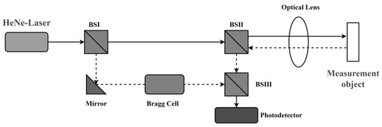
Figure 1.
Schematic diagram of the laser vibrometer.
The layout of the laser vibrometer weld plate defect detection system is shown in Figure 2. The laser vibrometer is mainly composed of an optical head and a control box. The optical head collects vibration signals, which are demodulated by the control box and transmitted to the computer via the A/D acquisition card. The host computer software, QuickSA4.0, then displays and stores the data to obtain the relationship between the amplitude and time changes. By processing the vibration signal, the corresponding vibration time–frequency characteristics of the welded plate are extracted, and then the vibration characteristics are compared and categorized to distinguish the differences between normal welded plates and various defective welded plates.
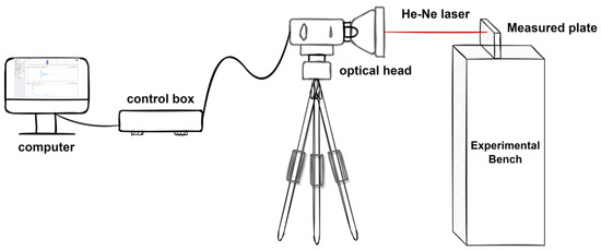
Figure 2.
Preparation and defect classification of experimental welded plates.
2.3. Research on Vibration Signal Processing Algorithms
It is known that, based on structural vibration characteristics, welded plate defects can be recognized by the structural natural frequency shift caused by defects or other features. In this paper, the vibration signal generated after the excitation of the welded plate is collected by a laser vibrometer for time–frequency feature extraction, which uses a traditional signal processing algorithm as a starting point. The theoretical derivation of the algorithm is explored, and simulations and analyses are conducted on the ideal transient signal model.
2.3.1. Limitations of Classical Time–Frequency Analysis Methods
For the signal acquired by the laser vibrometer, if it is processed by the traditional linear time–frequency analysis (TFA) method, it is closely related to the phase dictionary of the waveforms focused on the time–frequency domain, i.e.,
where the basis function represents the time–frequency (TF) displacement waveform. Because of the limitations of in TF, the TF characterization of the signal is restricted to being projected onto a square region called the Heisenberg box. As a result, the TFA method only provides a relatively coarse TF characterization when dealing with time-varying signals, and it is difficult to accurately capture and resolve transient features, especially when dealing with signals with rapidly changing states [20,21,22].
The collected vibration signals, as shown in Figure 3a, were analyzed using two classical algorithms in TFA: STFT (short-time Fourier transform) and WT (wavelet transform), and the results are shown in Figure 3b,c. For STFT, the researcher chose a Gaussian function as a moving window with a window length of 100 samples. For WT, the researcher used the Morlet function for this transient signal. It can be seen that the transient components in the TF plane are much more distributed in the time direction than in the original time series domain. Although the time-varying TF information can be obtained by the linear TF transform, it sacrifices the ability to pinpoint transient events.
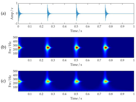
Figure 3.
(a) Signal time-domain diagram; (b) STFT transformation result; (c) WT transformation result.
2.3.2. Theoretical Implementation of Algorithm Optimization and Comparison of Simulation Results
In order to reduce the limitations of Heisenberg’s uncertainty principle, the simultaneous acquisition of time and frequency resolution in STFT and similar transformations that may be involved, as well as the better extraction of vibration signals with welded plate features for defect identification, was performed.
In this paper, we start our study with the framework of STFT, which is analyzed using the Dirac function with perfect time position properties. The expression of STFT is as follows:
where is the movable window and is the signal. The STFT basis function is shifted in the time domain while being modulated in the frequency domain to realize the extraction of transient features. Theoretically, the Dirac function is a generalized function on the real number line, characterized by having real values only at and an integral value of 1. Therefore, the Dirac function is an ideal model for signals with transient features. The Dirac signal representation is as follows:
A 200 Hz and , s sampling were used to illustrate the derivation process more intuitively here. The time waveform and spectrum of the Dirac signal are shown in Figure 4a,b, which correspondingly exhibit the optimal time resolution and the worst frequency resolution. The result of processing the signal with STFT is shown in Figure 4c, where the Dirac signal corresponds to an energy with an ideal temporal resolution but with a significant expansion in the TF plane. This indicates that, limited by Heisenberg’s principle of uncertainty, it is difficult to obtain both an extremely high time resolution and frequency resolution, even for the Dirac signal in the STFT method. To further investigate the TF energy distribution of the STFT results, Equation (3) is replaced by Equation (4) to obtain the following:
where , the energy distribution of the STFT result for the Dirac function, is expressed as follows:

Figure 4.
Simulation results under the ideal model based on the Dirac function: (a) dirac function signal at s; (b) spectrum; (c) STFT spectrogram; (d) slice of the spectrogram at Hz, i.e., ; (e) GD ; (f) slice of the GD at Hz, i.e., ; (g) TEO; and (h) results of the TET Test.
Through Equation (6), it can be seen that the window function is contracted in the time domain and the energy distribution of is concentrated at time and reaches its maximum at this time point . For further illustration, Figure 4d shows a slice of the STFT spectrum at the frequency Hz. The TF energy expands in the time direction.
In addition, the STFT of a Dirac function is composed of Dirac functions that have the same group delay (GD), with all GDs equal to . In order to accurately estimate the GD of each Dirac function , the frequency variables are first analyzed by derivatives. Therefore, the following equation can be stated:
Equation (8) follows from Equation (7). For any and , the of the 2D GD of STFT result (3) can be expressed as
The resultant imaging of Equation (8) is shown in Figure 4e, and, for a clearer interpretation of the GD, the results of the GD slices taken at the frequency are shown in Figure 4f. It is observed that in the TF interval , all the values of the 2D GD are equal to the values taken at s. However, the energy of the ideal TF representation of the signal in Equation (3) should be concentrated only at time . Therefore, the TF coefficients should be retained only at time , and the transient extraction operator (TEO) is further proposed as follows:
Included among these is
Capture
Equation (11) is a two-dimensional binarized representation of the TEO, which has a value of only 1 at time [see Figure 4g], and thus, the TF coefficients can be extracted using the TEO for at that point in time. Since Equation (9) has the function of transient extraction, the new TFA method using TEO is called transient extraction transformation (TET) and is denoted as follows:
From Equation (6), the energy of STFT spreads over a large area. The simulations are compared to analyze the energy distribution of the TET method in processing the Dirac function signal. The Dirac delta function is known to have the following properties:
Therefore, the energy distribution of the optimized TF representation is
Compared with the fuzzy energy distribution of the STFT result in Equation (6), the energy of the TET result in Equation (14) is highly concentrated and occurs only at the time, which satisfies the definition of the ideal TF representation of the Dirac function. The TET result of the Dirac signal is shown in Figure 4h, where the energy of the TF diffusion disappears and the retained TF coefficients have the same ideal time position as the Dirac function signal. The time and frequency resolution are optimized, and the interference between signal components is reduced.
2.3.3. Amplification and Reconstruction of TET Signals
In order to further investigate TET, the signal in Figure 4a was processed using the TET method and then enlarged, as shown in Figure 5, which indicates that the signal energy is more concentrated after TET processing and that the transient characteristics are more accurately characterized.
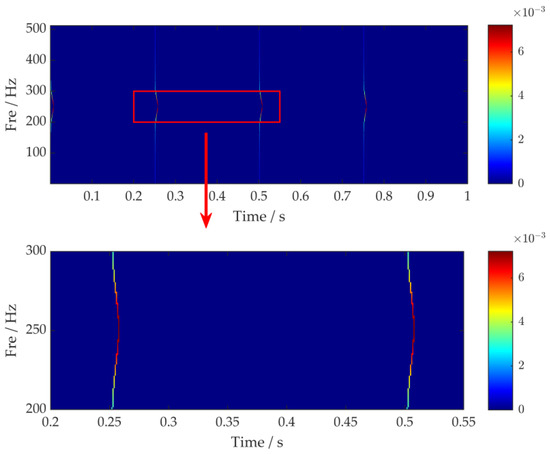
Figure 5.
Digital signals and scaling for TET representation.
It is now known that STFT has a signal reconstruction expression as follows:
The transient component is extracted from the transient transformation results with similar reconstructed expressions, given as follows:
By integrating more centralized TF results, the TET reconstruction is more suitable for extracting transient components than the STFT reconstruction, where the TET representation is as follows:
From the discrete Equation (17), it can be seen that TET and STFT have the same computational complexity, corresponding to the fact that the TET method also has the potential to be widely used in engineering.
3. Experiments
3.1. Experimental Design
Based on the preceding theoretical analysis and simulation, experimental measurements of defects in plate welds were carried out in this study. In the experiments, the same welding material was used to prepare welded plates with different defects by modifying the welding torch’s voltage, current, and technique. The dimensions of all experimental weld plates were 13 cm in length, 8 cm in width, 0.5 cm in thickness, and 0.8 cm in weld width. Figure 6 illustrates the experimental process, including the weld plate preparation site, the experimental plates, and enlarged views of their defective features.
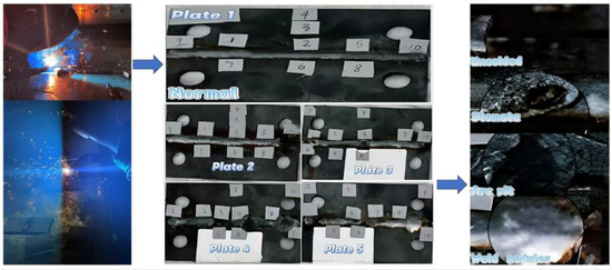
Figure 6.
Preparation and defect classification of experimental welded plates.
The experimental samples contained one normal weld plate and four weld plates with different defects, and the defect types were, in order, incomplete penetration, porosity, arc pit, and weld nodules overflow. As shown in Table 1, specifically, plate 1 is a normal welded plate; plate 2 has an incomplete penetration defect, characterized by the insufficient penetration of the welding material, leading to an inadequate backside weld and a visible weld seam; plate 3 is a porosity defect, caused by air infiltration during the welding process, resulting in a shallow depth and large-radius pores; plate 4 is an arc pit defect, caused by the instability of the electric arc or excessive cooling, insufficient weld material saturation, and a flat or slightly depressed weld seam surface; and plate 5 has a weld nodule overflow defect, caused by an excessive current or slow welding speed, characterized by an excessive solder or even overflow.

Table 1.
Experimental weld plate types.
Since the defects are small in size and difficult to accurately identify with the naked eye at a distance, a measurement system was designed to obtain vibration information. The object to be measured was fixed on the vise of the experimental bench, and the laser beam emitted from the optical hair of the laser vibration meter was utilized to align with the measurement point affixed with a reflective sheet and tapped periodically at the upper-right corner of the soldering plate. By collecting the vibration signal of the measured object and comparing it with the control experiment, the purpose of distinguishing the defects of the plate is achieved.
In order to verify the effect of the Doppler laser vibrometer on the detection of defects in welded plates, the experiment was designed to take fixed-point measurements on multiple welded plates and collect the corresponding vibration signals, after which the laser vibrometer was calibrated and verified. According to the JJG 676-2019 [23] “Vibrometer Calibration Regulations”, the calibration was conducted in the acoustic vibration laboratory of the Zhejiang Institute of Metrology and Research. The field measurement diagram is shown in Figure 7. The main equipment used in this calibration includes a standard vibration table, an accelerometer (vibration standard set), and a dynamic signal analyzer.
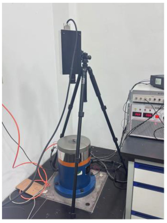
Figure 7.
Vibrometer measurement field calibration chart.
The measured calibration results are shown in Table 2, and the amplitude linearity of the laser vibrometer is summarized in Table 3, when the reference frequency is 80 Hz. It can be seen that the relative expanded uncertainty of the calibration results of the velocity amplitude error of the laser vibrometer used in the experiment is , . This shows that the measurement results have the advantages of high accuracy, high reliability, and suitability for high precision requirements. These advantages make the measurement results applicable in scientific research, engineering testing, quality control, and other fields.
Table 2.
Frequency-amplitude response.
Table 3.
Magnitude linearity.
3.2. Comparison of Experimental Signal Processing
The vibration signals of the tapped welded plate acquired by the laser vibrometer are processed in MATLAB for signal processing and comparative analysis. In this section, the algorithm implementation of the continuous wavelet transform (CWT) and short-time Fourier transform (STFT) on defective welded plates is shown sequentially. The horizontal axis of the image represents time, and the vertical axis represents frequency. The color represents magnitude: the closer the pixel point is to the light color (or warm colors, such as red), the larger the magnitude; the closer the pixel point is to the dark color (or cool colors, such as blue), the smaller the magnitude. The images of nine points at different locations in the intact plate 1 in Figure 8a and plate 4 with arc pit defects after CWT are presented in Figure 8b for comparison, with each image corresponding to three vibration measurement signals from a measurement point. Each subplot represents a time–frequency display of the vibration signal generated by three consecutive knocks at one measurement point of a plate. As shown in Figure 8, the distribution of the three tapping signals at the same measurement point on the same plate is similar, and the signals from a normal welded plate are concentrated in the 2 kHz to 3 kHz region with normal energy intensity, while a defective welded plate produces a large number of signals with low amplitude but high frequency in the region above 4 kHz. On the same welded plate, the characteristics of multiple tapping signals at the same location are basically the same, and the characteristics of signals at different locations on the same plate are also basically the same. This indicates that the time–frequency distribution patterns are similar for similar defect types. In conclusion, the defect types are different, and their corresponding wavelet time–frequency images are also different. The vibration signal images of different defective plates at the same measurement positions are similar, and the welded plate defects can be recognized initially. However, this WT identification is not stable, and signal spreading over a large area is not conducive for the efficient extraction of specific features. For example, when dealing with other defects, such as the porous defect represented in Figure 8c, the plate defect features can still be identified, but it is more difficult to intuitively distinguish the difference between the porosity in Figure 8c and the different features of the arc pit in Figure 8b. This indicates that the complexity of the WT extraction features, along with the interfering factors, is not conducive to differentiating between the different types of defects.
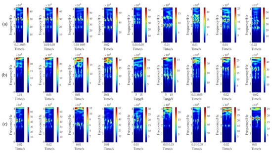
Figure 8.
Comparison of WT transformation results: (a) normal plate; (b) the plate containing arc pit defects; and (c) the plate containing porous defects.
The STFT is used to measure the same corresponding position of each plate, and three vibration signals are taken as a group to represent the signal characteristics of different welded plates, which include the signals of the normal plate, the incomplete penetration weld plate, the porous plate, the arc pit plate, and the weld nodule plate, in order from left to right in Figure 9a. By comparing the vibration signals of different plates at the same position after STFT processing, as shown in Figure 9b, it can be seen that the main frequency scale represented by normal plates is stable and concentrated in the range of 200 Hz to 300 Hz, while defective plates are significantly lower than this frequency range, being below 100 Hz. In the same scale, there are regular differences in the frequency ranges corresponding to different types of defects; for example, the main frequency range of the incomplete penetration weld plate is around 100 Hz, while the main frequency range of the porous welded plate is around 50 Hz, and so on. Compared with the results of the WT transformation, the STFT presents a more concentrated signal and can initially determine the type of defects. Whether it is WT transformation or STFT transformation, after processing, the signal characteristics are presented in the form of an image, which can be used to initially determine the defects. However, its resolution is limited by the size of the window and may exhibit spectral leakage; therefore, through a further optimization of the algorithm, the TET algorithm is used to analyze the vibration signals and detect defects.
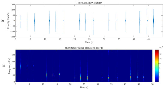
Figure 9.
Comparison of signal processing at the same location across different plates: (a) time-domain signal; (b) STFT transformation results.
The TET algorithm was first used to analyze the signal of the normal plate. The TF representation of the vibration signal at the first sampling point of normal plate 1 is shown in Figure 10a. The resultant repetitive transient shown by TFA extends the TF features to the TF plane, which provides more important information than a single time-domain analysis. In Figure 10c, the proposed TET method produces a centrally represented TF result, which provides better TF localization capability. The TF results of WT and STFT are weakly aggregated as compared to TET [see Figure 10b,d]. Similarly, although the spatial-time frequency transform (SST), which is designed to analyze the frequency characteristics of signals in space and time, is intended to yield sharper TF results, the SST results in Figure 10e are still unsatisfactory. In summary, limited by the Heisenberg measurement uncertainty principle, the STFT and WT cannot provide an energy-focused TF representation, and the SST does not give an energy-focused TF result. In contrast, in Figure 10c, the TET results, which appear to be much more clustered than in the other TFA methods, with a better high-resolution time–frequency analysis capabilities are presented.
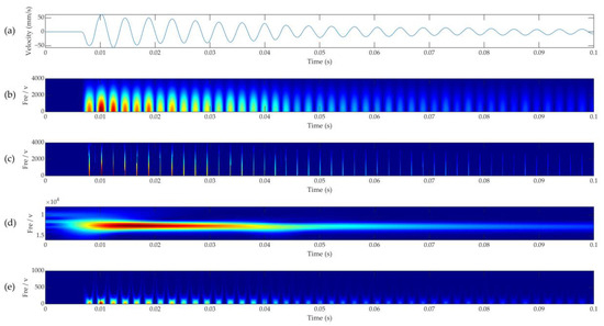
Figure 10.
(a) Normal ban111 waveform; (b) STFT results; (c) TET results; (d) WT results; (e) SST results.
3.3. Formatting of Mathematical Components and the Evaluation of Performance Indicators
In order to objectively evaluate the performance of the generated TF representations and effectively extract the transient components from different methods, two quantitative metrics, Rényi entropy and kurtosis, are introduced. These two metrics are used to evaluate the energy distribution properties and shape characteristics of the TF representation, respectively. The α-order Rényi entropy of the TF representation is defined as follows:
where the order of which is usually set to . The low Rényi entropy of the TF results indicates that the TET method generates a more centralized representation of the TF and provides a more accurate time-varying TF characterization.
Gaussian white noise, with a signal-to-noise ratio of 1 to 30 dB, is added to the numerical signal, as shown in Figure 11. The TFA methods (STFT, WT, SST, and TET) were used to process the noise-containing signals. The Rényi entropy of these TF representations generated by different TFA methods was calculated, as shown in Figure 11. This shows that the TET results have the smallest Rényi entropy at each noise level, indicating that TET exhibits strong robustness in processing noise-containing signals and is able to effectively display the most concentrated signal features.
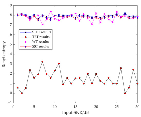
Figure 11.
Rényi entropy of TF results obtained by different TFA methods at different noise levels (S/N ratios of 1–30 dB).
Kurtosis, as a key indicator of signal crestiness, can keenly capture the transient features in the fault signal. The larger the kurtosis of the reconstructed result of the TFA method, the stronger the extraction capability of the method. The experimental results show that, as illustrated in Figure 12, with the gradual increase in the external noise level, the kurtosis value of the original signal decreases, which affects the extraction quality of the transient features of the signal. However, under the same noise level, the kurtosis value of the TET recovered signal always maintains at a high level, which demonstrates a stronger transient feature retention capability compared to the original signal, and it is also able to effectively extract the transient features of the signal in a noisy environment.
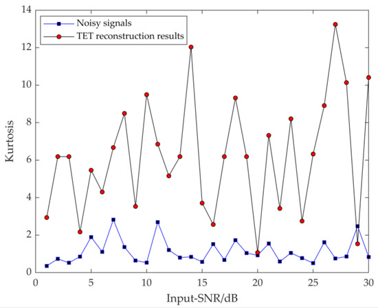
Figure 12.
Kurtosis at different noise levels (signal-to-noise ratio of 1–30 dB).
Table 4 shows the Rényi entropy values of several TF analysis results, and this quantitative metric intuitively verifies the superiority of the method proposed in this paper in terms of TF localization capability.
Table 4.
Rényi entropy corresponding to TF results.
In addition, Table 5 evaluates the efficiency of the above TFA methods in practical applications, and the processing time of the TET method is within 1 s, indicating a high level of efficiency as well.
Table 5.
Processing time of TFA methods for vibration signals.
Further, the transient components extracted by the TET method are significantly improved, in terms of the transient characteristics shown in Figure 13b, compared to the original signal (see Figure 13a), which are closer to the real characteristics of the resulting vibration signal.
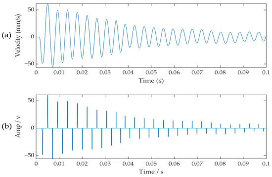
Figure 13.
(a) Raw signal; (b) transient component extraction using the TET method.
In order to further study the application of the TET algorithm in the defect detection of welded plates, the center positions of the measurement signals (ban121, ban221, ban331, ban431, and ban541) were used as representatives of all the measurement points of the five plates for the experiments. The actual point map is shown in Figure 6, and the experimental signal acquisition for each plate covered nine positions, and three tapping experiments were conducted at each position, totaling 27 × 5 sets of characteristic signal data. The naming rules for the collected plate signals follow the logic of “plate number + point number + vibration signal generation sequence number”. The placement of the data measurement points follows the principles of traversing the plate, close proximity, proximity to the weld seam, and center symmetry.
Section 3.2 shows that the STFT is more effective in processing vibration signals for defect identification. By improving the algorithm, the researcher compares the image effects of all the points at the same location in different welded plates under the influence of STFT and TET. The results show that the signal characteristics within the same plate are basically the same, and the signals at different locations on the same plate have a high degree of similarity. Therefore, according to the principle of measurement point arrangement, the measurement signal at the center position of each plate is selected to represent the defective features of the corresponding welded plate. The different defective feature signals are displayed in time–frequency diagrams, such as in Figure 14 and Figure 15, for further comparison and analysis.
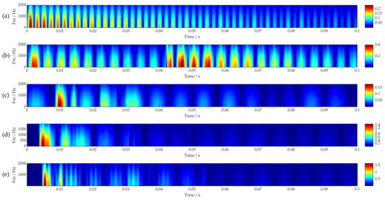
Figure 14.
STFT effect diagram: (a) ban121; (b) ban221; (c) ban331; (d) ban431; and (e) ban641.
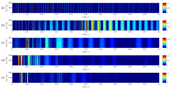
Figure 15.
TET effect diagram: (a) ban121; (b) ban221; (c) ban331; (d) ban431; and (e) ban641.
As shown in Figure 14, the vibration signals of the five welded plates demonstrated obvious differences in their features after STFT processing. The signal features corresponding to different plates vary significantly, but the signals are poorly aggregated, resulting in more frequency components and dispersion in the spectrogram, which is detrimental to feature extraction and may increase the risk of misclassification. In contrast, Figure 15 demonstrates the features of the vibration signals of the same five welded plates after TET processing. The results show that the signals from the experimental plates exhibit a better performance in terms of energy concentration, high peaks, transient component decomposition, and extraction, even with different defects.
Analyzing the frequency change and amplitude change in Figure 15, the duration of the tapping signal is 0.1 s. The change in amplitude follows the energy decay law, but there are regular differences in decay time and amplitude change for different types of welded plates. Figure 15a represents the time–frequency diagram of the normal plate, where the signal energy is mainly concentrated between 0.002 and 0.04 s, with an amplitude close to 0.1, starting to decay from 0.02 s. The decay amplitude and rate are relatively smooth, showing a strong signal aggregation and regularity. Figure 15b represents the time–frequency diagram of the incomplete penetration weld plate, where the signal rapidly attenuates in 0.04 s, followed by a trend of initial enhancement, and then attenuation between 0.04 and 0.1 s. The signal energy is mainly concentrated at 0.05 s, with an amplitude greater than 0.1, and the energy density is higher in the attenuation stage. Figure 15c represents the time–frequency diagram of the porous-welded plate, where the signal energy gathers at 0.01 s, with an amplitude of 0.05, and the subsequent decay phase has a smaller amplitude and high density. Figure 15d represents the time–frequency diagram of the arc pit weld plate, with more high-amplitude energy, mainly concentrated near 0.005 s, with an amplitude as high as 0.4, rapidly decaying from 0.01 s, with a short decay completion time. Figure 15e represents the time–frequency diagram of the weld nodule plate, with less high-amplitude energy, appearing from 0.005 s to 0.01 s, with an amplitude as high as 0.5, and the energy rapidly decaying, with a shorter decay completion time.
In summary, by comparing the time–frequency diagrams, the normal welded plate maintains good regularity and integrity, while the four different defects show distinct time–frequency distribution patterns. This difference provides an important basis for defect identification, and the time–frequency diagrams processed using the TET algorithm can extract and demonstrate the signal characteristics of the welded plates more effectively.
4. Discussion
The laser vibrometer shows great potential in defect detection, but the traditional time–frequency analysis method has limitations in dealing with such high-resolution signals. In view of the above problems, this paper applies the laser vibrometer to optimize the algorithm for the vibration signals collected from the welded plate, which achieves a better aggregation in vibration signal extraction.
The algorithm adaptability optimization is based on the use of classical WT and STFT to process the experimental welded plate vibration signal. A comparison reveals that the STFT-processed signal is more aggregated, and the defective features are distinguishable, stable, and obvious. The more suitable STFT algorithm is selected, but because the resolution of the STFT algorithm is constrained by the window size, an improved version of the STFT algorithm is proposed. The optimized TET algorithm improves the limitations of the traditional STFT in time–frequency resolution by means of adaptive windowing, combining a multi-resolution analysis with enhanced transient characteristics, making it more effective in processing complex signals. As demonstrated in this paper, Figure 8 presents the overall effect graphs of all vibration signals on normal, arc-pit, and porous plates (3 categories) after WT changes, illustrating the characteristics that WT can effectively recognize, but the recognition is not stable. Figure 9 shows a representative local vibration signal corresponding to the same location on all experimental plates (5 categories) after the STFT changes, demonstrating that the STFT can distinguish the defects of the welded plate, but its resolution is limited by the size of the window.
Therefore, based on the optimization of the STFT algorithm, the optimized TET algorithm is applied to the vibration analysis of welded steel plates. From the results in Figure 10, combined with the algorithm comparison chart and the indicators in Chapter 3, the superiority of the TET algorithm in analyzing the vibration signals of welded plates collected by the laser vibrometer is further illustrated. As observed in Figure 15, the TET algorithm can extract more aggregated signal characteristics, and defects in the welded plates can be initially differentiated from the spectrogram. This study provides a reference for future studies on feature extraction and the defect detection of welded plates using laser vibrometers.
5. Conclusions
In this paper, the application of the time–frequency analysis (TFA) method based on a laser vibrometer in the defect detection of welded plates is investigated, providing new ideas in vibration signal processing. By optimizing the STFT algorithm to obtain the transient extraction transform algorithm (TET), the localization analysis technique allows the TET to overcome the limitations of the fixed window while reducing the adverse effects of Heisenberg’s uncertainty principle. This provides a high-resolution time–frequency analysis that exhibits strong robustness to noise. By applying the TET algorithm to the vibration signal processing of welded plate defect detection, not only are the redundant and ambiguous components in the time–frequency plane effectively eliminated, but the information closely related to the transient characteristics of the signals is accurately retained. This improves the accuracy of the time–frequency analysis and the ability to capture transient characteristics. This study enriches the theoretical framework of time–frequency analysis and provides new insights for defect detection in welded plates.
Author Contributions
Conceptualization, X.X. and Y.D.; methodology, Y.D.; software, D.Y.; validation, X.X., Y.D. and J.W.; formal analysis, L.Z.; investigation, Y.D.; resources, X.X.; data curation, Y.D.; writing—original draft preparation, Y.D.; writing—review and editing, Y.D.; visualization, Y.D.; supervision, X.X.; project administration, Y.D.; funding acquisition, X.X. All authors have read and agreed to the published version of the manuscript.
Funding
This study was supported by the Natural Science Foundation of Zhejiang Province under Grant No. LY19F050008.
Data Availability Statement
Some of the data provided in this study have been in the main text, due to the commercial privacy considerations involved, the other data are not available to the public for the time being, if there is a special need you can ask the corresponding author of this paper for other relevant data.
Conflicts of Interest
The authors declare no conflict of interest.
References
- Madhav, M.; Ambekar, S.S.; Hudnurkar, M. Weld defect detection with convolutional neural network: An application of deep learning. Ann. Oper. Res. 2023, 343, 1–24. [Google Scholar] [CrossRef]
- Sun, J.; Li, C.; Wu, X.-J.; Palade, V.; Fang, W. An effective method of weld defect detection and classification based on machine vision. IEEE Trans. Ind. Inform. 2019, 15, 6322–6333. [Google Scholar] [CrossRef]
- Rothberg, S.J.; Allen, M.; Castellini, P.; Di Maio, D.; Dirckx, J.; Ewins, D.; Halkon, B.J.; Muyshondt, P.; Paone, N.; Ryan, T.J.O.; et al. An international review of laser Doppler vibrometry: Making light work of vibration measurement. Opt. Lasers Eng. 2017, 99, 11–22. [Google Scholar] [CrossRef]
- Vavilov, V.; Karabutov, A.; Chulkov, A.; Derusova, D.; Moskovchenko, A.; Cherepetskaya, E.; Mironova, E. Comparative study of active infrared thermography, ultrasonic laser vibrometry and laser ultrasonics in application to the inspection of graphite/epoxy composite parts. Quant. Infrared Thermogr. J. 2020, 17, 235–248. [Google Scholar] [CrossRef]
- Segers, J.; Kersemans, M.; Hedayatrasa, S.; Calderon, J.; Van Paepegem, W. Towards in-plane local defect resonance for non-destructive testing of polymers and composites. NDT E Int. 2018, 98, 130–133. [Google Scholar] [CrossRef]
- Szeleziński, A.; Muc, A.; Murawski, L.; Kluczyk, M.; Muchowski, T. Application of laser vibrometry to assess defects in ship hull’s welded joints’ technical condition. Sensors 2021, 21, 895. [Google Scholar] [CrossRef]
- Hasheminejad, N.; Vuye, C.; Van den bergh, W.; Dirckx, J.; Vanlanduit, S. A comparative study of laser Doppler vibrometers for vibration measurements on pavement materials. Infrastructures 2018, 3, 47. [Google Scholar] [CrossRef]
- Derusova, D.A.; Vavilov, V.P.; Druzhinin, N.V.; Shpil’noi, V.Y.; Pestryakov, A.N. Detecting Defects in Composite Polymers by Using 3D Scanning Laser Doppler Vibrometry. Materials 2022, 15, 7176. [Google Scholar] [CrossRef]
- Gherlone, M.; Mattone, M.; Surace, C.; Tassotti, A.; Tessler, A. Novel vibration-based methods for detecting delamination damage in composite plate and shell laminates. Key Eng. Mater. 2005, 293, 289–296. [Google Scholar] [CrossRef]
- Zeng, H.; Ye, F.; Cai, J.; Xu, Y. A method for assessing the operational status of a microseismic monitoring system using energy distribution changes of observed data. J. Geophys. Eng. 2024, 21, 1379–1391. [Google Scholar] [CrossRef]
- Farrar, C.R.; Doebling, S.W.; Nix, D.A. Vibration–based structural damage identification. Philos. Trans. R. Soc. Lond. Ser. A Math. Phys. Eng. Sci. 2001, 359, 131–149. [Google Scholar] [CrossRef]
- Della, C.N.; Shu, D. Vibration of delaminated composite laminates: A review. Appl. Mech. Rev. 2007, 60, 1–20. [Google Scholar] [CrossRef]
- Gigerenzer, G.J.B. What are natural frequencies? BMJ 2011, 343, d6386. [Google Scholar] [CrossRef]
- Pastor, M.; Binda, M.; Harčarik, T. Modal assurance criterion. Procedia Eng. 2012, 48, 543–548. [Google Scholar] [CrossRef]
- Morassi, A. Damage detection and generalized Fourier coefficients. J. Sound Vib. 2007, 302, 229–259. [Google Scholar] [CrossRef]
- Hajela, P.; Soeiro, F.J. Structural damage detection based on static and modal analysis. AIAA J. 1990, 28, 1110–1115. [Google Scholar] [CrossRef]
- Hagood, N.; von Flotow, A. Damping of structural vibrations with piezoelectric materials and passive electrical networks. J. Sound Vib. 1991, 146, 243–268. [Google Scholar] [CrossRef]
- Koszewnik, A.; Grześ, P.; Walendziuk, W. Mechanical and electrical impedance matching in a piezoelectric beam for Energy Harvesting. Eur. Phys. J. Spéc. Top. 2015, 224, 2719–2731. [Google Scholar] [CrossRef]
- Kang, T.; Moon, S.; Han, S.; Jeon, J.Y.; Park, G. Measurement of shallow defects in metal plates using inter-digital transducer-based laser-scanning vibrometer. NDT E Int. 2019, 102, 26–34. [Google Scholar] [CrossRef]
- Cristalli, C.; Paone, N.; Rodríguez, R. Mechanical fault detection of electric motors by laser vibrometer and accelerometer measurements. Mech. Syst. Signal Process. 2006, 20, 1350–1361. [Google Scholar] [CrossRef]
- He, D.; Cao, H.; Wang, S.; Chen, X. Time-reassigned synchrosqueezing transform: The algorithm and its applications in mechanical signal processing. Mech. Syst. Signal Process. 2019, 117, 255–279. [Google Scholar] [CrossRef]
- Yu, G.; Wang, Z.; Zhao, P. Multisynchrosqueezing transform. IEEE Trans. Ind. Electron. 2018, 66, 5441–5455.qi. [Google Scholar] [CrossRef]
- Huang, S.; Geng, Y.; Han, Y.; Gu, M. Design of Shocks & Vibrations Monitoring System for Long Distance Transportation in Confined Spaces. In Proceedings of the 2023 China Automation Congress (CAC), Chongqing, China, 17–19 November 2023; pp. 4886–4892. [Google Scholar]
Disclaimer/Publisher’s Note: The statements, opinions and data contained in all publications are solely those of the individual author(s) and contributor(s) and not of MDPI and/or the editor(s). MDPI and/or the editor(s) disclaim responsibility for any injury to people or property resulting from any ideas, methods, instructions or products referred to in the content. |
© 2024 by the authors. Licensee MDPI, Basel, Switzerland. This article is an open access article distributed under the terms and conditions of the Creative Commons Attribution (CC BY) license (https://creativecommons.org/licenses/by/4.0/).