Experimental Research on the Correction of Vortex Light Wavefront Distortion

Abstract

Wavefront distortion occurs when vortex beams are transmitted in the atmosphere. The turbulence effect greatly affects the transmission of information, so it is necessary to use adaptive optical correction technology to correct the wavefront distortion of the vortex beam at the receiving end. In this paper, a method of vortex wavefront distortion correction based on the deep deterministic policy gradient algorithm is proposed; this is a new correction method that can effectively handle high-dimensional state and action spaces and is especially suitable for correction problems in continuous action spaces. The entire system uses adaptive wavefront correction technology without a wavefront sensor. The simulation results show that the deep deterministic policy gradient algorithm can effectively correct the distorted vortex beams and improve the mode purity, and the intensity correlation coefficient of single-mode vortex light can be increased to about 0.88 and 0.69, respectively, under weak turbulence and strong turbulence, and the intensity coefficient of weak-turbulence multi-mode vortex light can be increased to about 0.96. The experimental results also show that the adaptive correction technology based on the deep deterministic policy gradient algorithm can effectively correct the wavefront distortion of vortex light.

1. Introduction

With the increasing demand for modern communication services, improving communication rates and expanding channel capacity have become common requirements. As the carrier of information transmission, light not only has a high available bandwidth, but also has the advantages [1] of high speed, large capacity, low cost, and strong confidentiality. The vortex beam brings these huge advantages to optical communication. As mentioned above, free-space optical communication uses a light beam as the carrier of information. When the light beam is transmitted in the atmospheric channel, the atmospheric channel is time-varying due to the random fluctuations in the atmospheric refractive index, which are very unfavorable for information transmission in the communication system. When vortex beams are transmitted in the atmosphere, wavefront distortion will occur, the light intensity distribution will change, phase distortion will occur, crosstalk will occur between the multiplexed Orbital Angular Momentum (OAM) modes, and the mode purity will decrease. The turbulence effect greatly affects the transmission of information, so it is necessary to use adaptive optical correction technology to correct the wavefront distortion of the vortex beam distorted by atmospheric turbulence at the receiving end. Therefore, scholars in China and internationally have carried out a lot of research work on adaptive optics (AO) correction technology to suppress turbulence.

For wavefront distortion correction in vortex beams, scholars in China and internationally have carried out a lot of research on adaptive wavefront correction technology in vortex beams [2,3]. The main technology includes the Shack–Hartmann (SH) method [4,5,6] for the Shack–Hartmann wavefront sensor. There are two main wavefront sensorless methods: the Gerchberg–Saxton (GS) algorithm [7,8,9] and the Stochastic Parallel Gradient Descent (SPGD) [10,11,12,13]. The above conventional vortex beam distortion correction technology has certain shortcomings. The correction method based on the Shack–Hartmann wavefront sensor is costly and adds a complex coaxial system. The method based on the combination of a surface array detector and the GS or SPGD algorithm has the problems of a long system response time and insufficient correction accuracy. We found that deep neural networks, or networks containing multiple layers of neurons, have made major breakthroughs in several fields and even surpassed human levels in some tasks. Deep neural networks are also known as deep learning. With the success of deep learning in various fields, researchers began to use deep learning as a phase extraction algorithm. Y. Jin et al. [14] introduced deep learning-based wavefront sensing technology into adaptive optical systems, which could effectively compensate for the distortion brought by biological tissues. In addition to distortion sources such as biological tissues, atmospheric turbulence, as a complex aberration, can also be extracted by deep learning. H. Ma et al. [15] used deep learning to extract atmospheric turbulence information from the intensity distribution of aberrations. J. Gao et al. [16]. applied deep learning to mitigate the effects of atmospheric turbulence on images. In order to further study the ability of deep learning to extract atmospheric turbulence, Q. Tian et al. [17] showed that deep learning can directly extract turbulence aberrations from intensity images under different turbulence intensifies and successfully applied it in adaptive optical systems. Lillicrap et al. [18] extended the idea of Deep Q Networks (DQN) and combined the ideas and methods in DQN with Deterministic Policy Gradient (DPG). Using an off-line policy training method with a replay buffer, while using a separate target network, a Deep Deterministic Policy Gradient (DDPG) algorithm is proposed. DDPG combines the actor–critic framework with a neural network function approximation method. The empirical playback mechanism is used, and the batch normalization technique is utilized. The application of these techniques enables the deep deterministic strategy gradient algorithm to learn in a high-dimensional state and action space. Deep deterministic strategy gradient algorithms can be applied to continuous action space problems that DQN struggle to handle and can achieve better performance than DQN with less experience than DQN. On this basis, this paper refers to the classical adaptive optics system, adopts the vortex optical adaptive wavefront correction technology without a wavefront sensor, takes the DDPG algorithm as the adaptive algorithm, takes the Deformation Mirror (DM) as the wavefront corrector, and combines the simulation and experimental results. It shows that the adaptive correction technology using the DDPG algorithm can effectively perform the wavefront distortion correction of vortex beams.

2. Basic Theory

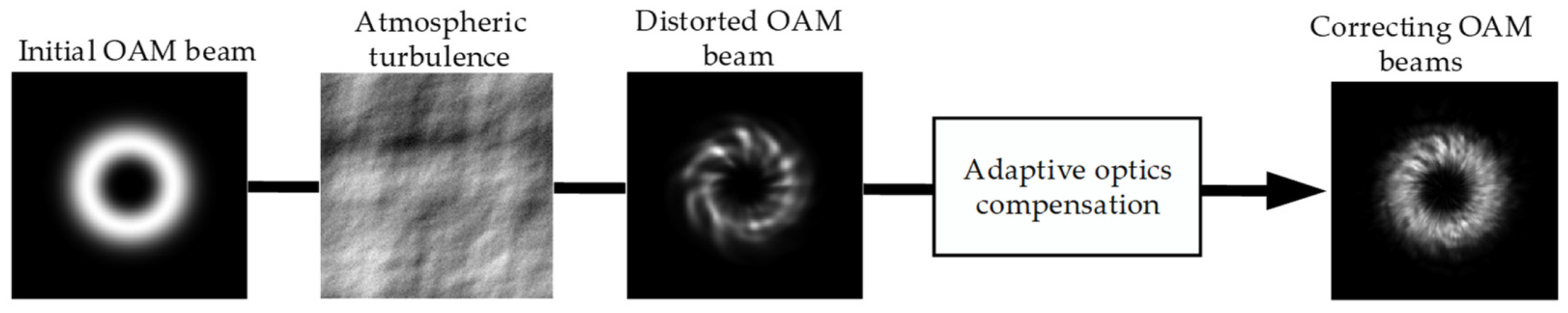
2.1. Adaptive Optics Wavefront Correction Techniques in Vortex Beams

The Laguerre–Gaussian (LG) beam is the most widely used beam in the free-space vortex optical communication system at present. The mathematical expression [19] of the Laguerre–Gaussian beam can be obtained by solving the Helmholtz equation in a cylindrical coordinate system and performing paraxial approximation along the beam propagation direction.

$$\begin{array}{cc}L{G}_{p,l}\left(r,\phi ,z\right)=\hfill & \sqrt{{\displaystyle \frac{2p!}{\pi \left(p+\left|l\right|\right)!}}}\ast {\displaystyle \frac{1}{\omega \left(z\right)}}\ast {\left({\displaystyle \frac{r\sqrt{2}}{\omega \left(z\right)}}\right)}^{\mid l|}\ast exp\left({\displaystyle \frac{-r^2}{{\omega }^2\left(z\right)}}\right)\ast L_p^{\left|l\right|}\ast \left({\displaystyle \frac{2r^2}{{\omega }^2\left(z\right)}}\right)\hfill \\ \hfill & \hfill \ast exp\left(-il\phi \right)\ast exp\left({\displaystyle \frac{ik{r}^{2}z}{2\left(z^2+z_R^2\right)}}\right)\ast exp\left[-i\left(2p+\left|l\right|+1\right)arctan\left({\displaystyle \frac{z}{z_R}}\right)\right]\end{array}$$

(1)

where r is the radial distance of the beam propagation; $\phi$ is the azimuth angle; $z$ is the propagation distance; $\omega \left(z\right)$ is the spot radius of the equal phase surface of the LG beam at the propagation distance $z$; $\mathsf{\omega }\left(z\right)={\omega }_0\sqrt{1+{\left(z/z_R\right)}^2}$, where R represents the waist radius ${\omega }_0$ of the LG beam; $z_R=\pi {\omega }_0^2/\lambda$, where $\lambda$ is the beam wavelength; $k=2\pi /\lambda$ is the wave number; $\left(2p+\left|l\right|+1\right)arctan\left(z/z_R\right)$ represents the Gouy phase; $L_p^{\left|l\right|}$ is the Laguerre polynomial; $l$ is the topological charge; and $p$ is the radial index.

Adaptive optical correction technology emerged in the 1970s and has been widely [20,21,22] used in astronomy and military fields. The traditional adaptive optical correction system can be divided into wavefront sensor adaptive correction system and wavefront sensorless adaptive correction system. This paper adopts the wavefront sensing adaptive system, of which the system structure is shown in Figure 1. Its principle is to directly obtain some specific light intensity distribution information for the distorted OAM beam and then directly use the correction algorithm to calculate the control signal of the correction voltage of the deformed mirror according to the light intensity information of the distorted OAM beam, so as to achieve the purpose of correcting the distorted OAM beam.

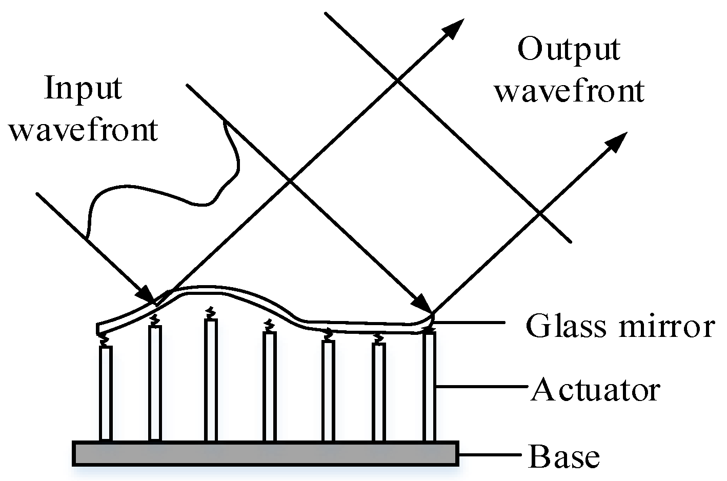
2.2. Deformable Mirror

As the main executive mechanism of an adaptive optical system to improve a distorted wavefront, the DM functions like a filter. According to the output voltage signal of the wavefront controller, the DM drives each unit to produce a conjugate surface with the phase of the incident distorted wavefront. By changing the transmission optical path difference in the incident distorted wavefront, the beam fluctuation caused by atmospheric turbulence is compensated. Therefore, the wavefront corrected by the DM is approximately a plane wave, which achieves the purpose of correcting the wavefront distortion. As can be seen in Figure 2 [23], the DM is composed of a number of drivers arranged according to the law, and each driver is controlled by changing the applied voltage. Applying different control voltages to each actuator unit will ultimately control the DM to produce the desired surface shape.

The mirror of a continuous surface DM is acted on by all drivers together. In general, the effect of voltage on the deformation mirror driver can be regarded as linear [24]. Therefore, the compensation phase total shape variable generated by the DM can be expressed as follows:

$$\psi \left(\begin{array}{c}r\end{array}\right)={{\displaystyle \sum }}_{i=1}^N{V}_j{S}_j\left(\begin{array}{c}r\end{array}\right)$$

(2)

In this formula, N represents the number of DM actuators; based on the correspondence between the actuator spacing and the coherence length of atmospheric turbulence, this paper uses a 69-element DM to correct the wavefront distortion, achieving a good trade-off between the wavefront correction effect and system complexity. $V_j$ is the control voltage of the $j$-th actuator, and $S_j\left(\begin{array}{c}r\end{array}\right)$ is the influence function of the $j$-th actuator, which follows a Gaussian distribution and can be expressed as

$$S_j\left(r\right)=S_j\left(x,y\right)=exp\left\{ln\omega {[{\displaystyle \frac{1}{d}}\sqrt{{\left(x-x_j\right)}^2+{\left(y-y_j\right)}^2}]}^{\alpha }\right\}$$

(3)

where $\omega$ is the cross-linking value of the drive. According to Pearson’s experience data, the ideal cross-linking value is between 5% and 12%, and the actual measured cross-linking value is 85%. $x_j,y_j$ represent the horizontal and vertical coordinates of the $j$-th actuator, respectively, $d$ = 1.55 mm is the normalized distance between the actuators on the DM, and $\alpha$ is the Gaussian exponent.

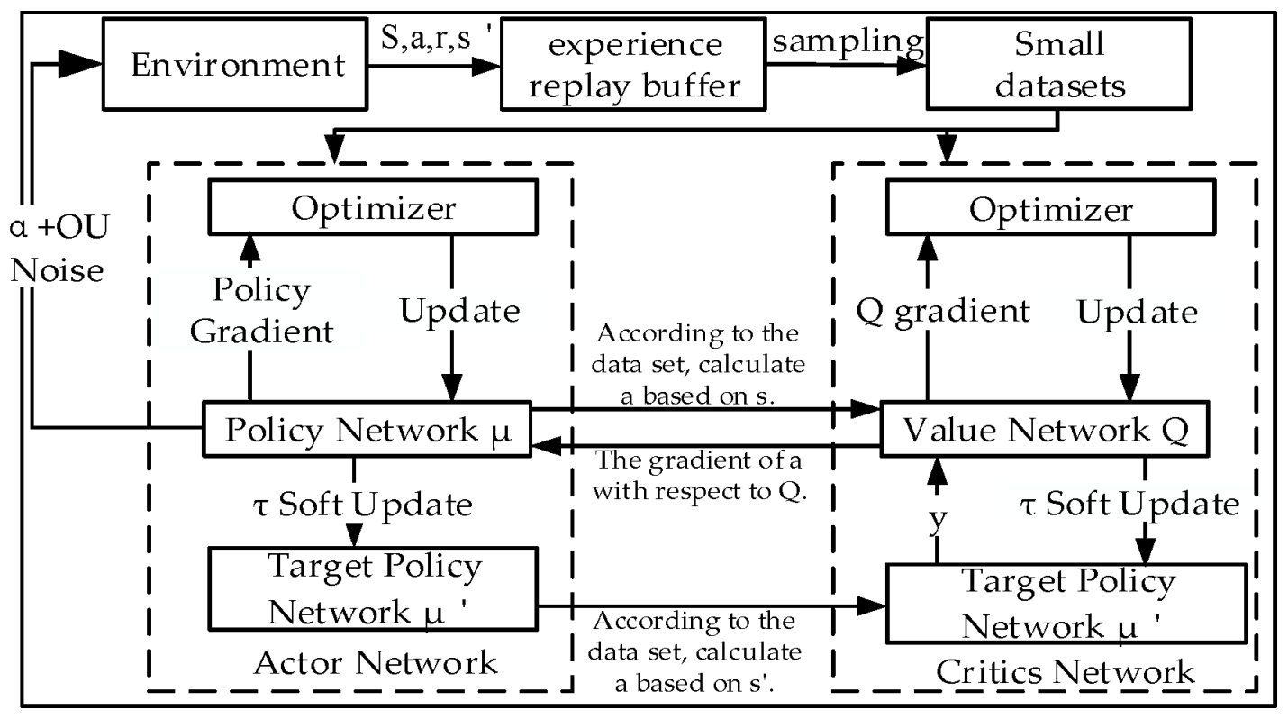
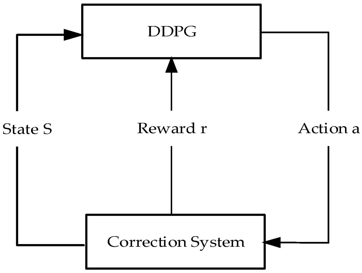
2.3. Corrective Principles of DDPG Algorithms

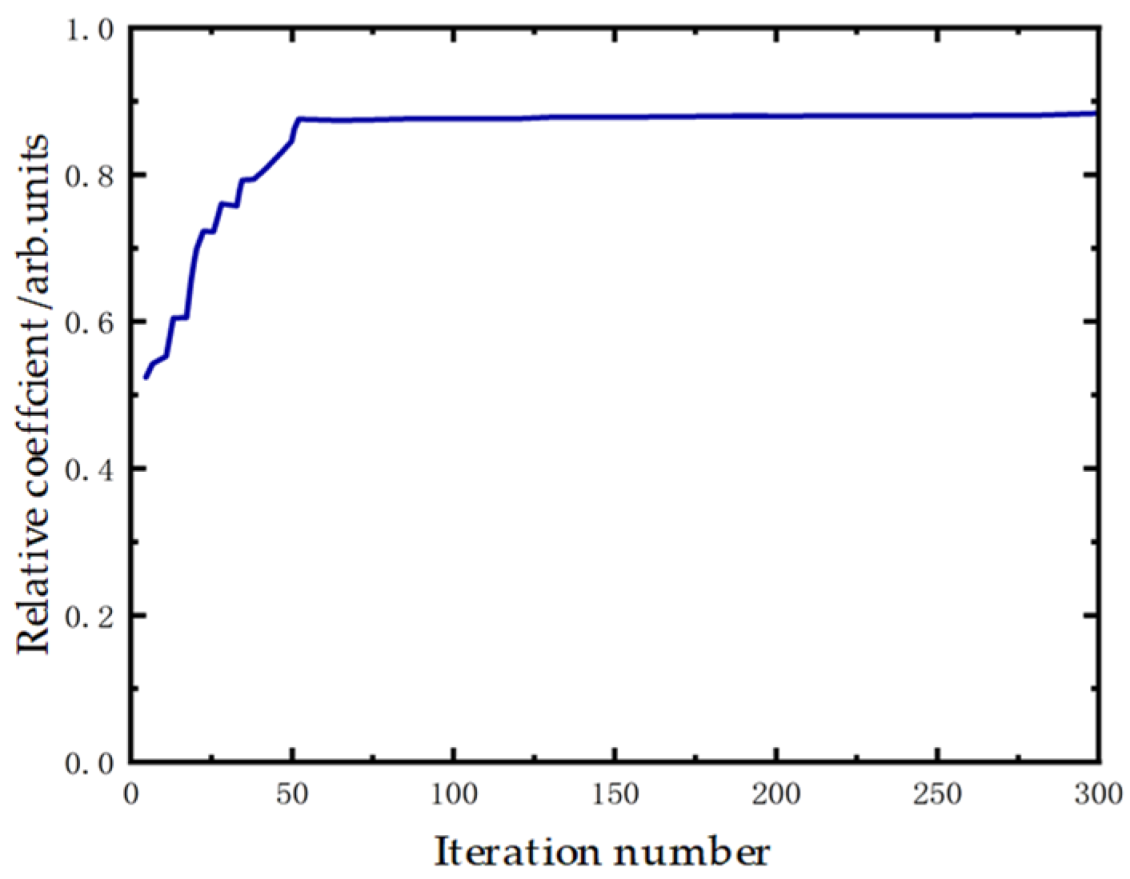
The DDPG algorithm adopts the actor–critic algorithm as its basic structure and uses an experience replay mechanism to eliminate the correlation and dependence among sample data. It also uses a dual network model design for both the policy function (actor) and the value function (critic), making the learning and training process of the algorithm more easily convergent and stable. The flowchart of the DDPG algorithm is shown in Figure 3 [25]. The main body of the model consists of four neural networks: the policy network, the target policy network, the value network, and the target value network, while the specific network structure depends on the target problem and computing resources and satisfies the dimensions of input and output.

In the DDPG algorithm, the action $a_t$ of the agent at each time step is determined by the deterministic policy $\mu$; that is, $a_t$ = $\mu \left(s_t\right)$. At the same time, it is approximated by a neural network called the policy network, $a=\mu \left(s,{\theta }^{\mu }\right)$. The value function $Q^{\mu }$ is still defined by the Bellman equation and is approximated by a neural network known as the value network $Q\left(s,a,{\theta }^Q\right)$. The purpose of the agent’s exploration is to find potentially better strategies. Therefore, the DDPG algorithm introduces an Ornstein–Uhlenbeck stochastic process as noise, referred to as the behavior policy $\beta$, which generates a distribution function ${\rho }^{\beta }$ for the state set.

In the DDPG algorithm, the action, a, taken by the agent at each time step is determined by a deterministic action policy u, i.e., a = ust, while it is approximated by a neural network called the policy network, a = us0. The value function Q is still defined by the Bellman equation, while it is approximated by a neural network called the value network Qsa0. The goal of the agent’s exploration is to find potentially better strategies, so the DDPG algorithm introduces an Ornstein–Uhlenbeck stochastic process as noise, called the behavior policy, b, which generates a distribution function for the state set, pb.

In the deep deterministic strategy gradient algorithm, the agent can constantly interact with the environment and make a decision, judge whether the decision is feasible according to the return obtained after the action, then find the optimal action strategy under the current state by continuous learning and decision-making, and then achieve the control goal. The deep deterministic strategy gradient algorithm introduces the actor–critic method, adopts off-policy actor–critic methods, and uses function approximation method to estimate the value function [26]. The gradient formula of the deterministic strategy gradient of different strategies is as follows:

$${\nabla }_{\theta }{J}_{\beta }\left({\mu }_{\theta }\right)=E_{s-{\rho }^{\beta }}\left[{\nabla }_{\theta }{\mu }_{\theta }\left(s\right){\nabla }_a{Q}^{\mu }\left(s,a\right){|}_{a={\mu }_{\theta }\left(s\right)}\right]$$

(4)

When the state is S, strategy $\theta$ is adopted, and the deterministic action $a$ of the determined strategy ${\mu }_{\theta }\left(s\right)$ is determined. For the deterministic strategy, a large number of samples need to be taken in the state space with sampling strategy $\beta$, and the integral of the state distribution is taken, the mean of which can approximate the expected value. In order to reduce the Markovian correlation between sampled data, the DDPG algorithm draws on the DQN algorithm, employing experience replay and separate target networks to approximate the action-value function and the deterministic policy. Experience replay refers to the process in reinforcement learning where an agent stores the current state $s_t$, current action $a_t$, reward $r_t$, and the next state $s_{t+1}$ in the database $R$. Then, random data ($s_k$,$a_k$,$r_k$,$s_{k+1}$) are uniformly sampled from the database to train the neural network, thereby breaking the correlation between data points. An independent target network is set up to correct biases, further reducing correlations and making the results more accurate, as shown in Equation (2), where $\gamma$ is the discount factor.

$$y_k=r_k+\gamma Q^{\prime }(s_{k+1},{\mu }^{\prime }\left(s_{k+1}\left|{\theta }^{{\mu }^{\prime }})\right|{\theta }^{Q^{\prime }}\right)$$

(5)

For the AC network parameters in the DDPG algorithm, independent networks are used for updates. The actor current network and the critic network are responsible for the iterative updates to the policy network parameters ${\theta }^Q$ and the value network parameters ${\theta }^{\mu }$, respectively. Based on the sampled policy gradient $\nabla {\theta }^{\mu }\mu {|}_{s_k}$, the returns generated by the actions are maximized to update the actor network parameters ${\theta }^Q$, as shown in Equation (6), to predict the optimal actions, given a state. The mean squared error loss function L_min is used to minimize the updates to the critic network parameters ${\theta }^{\mu }$, as shown in Equation (7), making the estimates closer to the target Q-value.

$${\nabla }_{{\theta }^{\mu }}\mu {|}_{s_k}\approx {\displaystyle \frac{1}{N}}{{\displaystyle \sum }}_k{\nabla }_{a}Q\left(s,a|{\theta }^Q\right){|}_{s=s_k,a=\mu \left(s_k\right)}{\nabla }_{{\theta }^{\mu }}\mu \left(s|{\theta }^{\mu }\right){|}_{s_k}$$

(6)

$$L_{min}={\displaystyle \frac{1}{N}}{{\displaystyle \sum }}_k\left(y_k-Q{\left(s_k,a_k|{\theta }^Q\right)}^2\right)$$

(7)

The soft update method is used to update the target network parameters in a soft manner, which is an important technology in the DDPG algorithm for stabilizing the learning process. In DDPG, soft update is mainly used for parameter updates in the target network. The target network is a delayed copy of the current network, and its parameters are not updated in real time, but gradually approached in a specific proportion (usually a small positive number, such as t = 0.001) towards the parameters of the current network. This update method helps reduce instability in the learning process because it avoids drastic changes in the target network parameters, making the learning signal smoother and more stable. That is, part of the parameters ${\theta }^Q$ and ${\theta }^{\mu }$ of the current network are partially migrated and copied to the corresponding parameters ${\theta }^{Q^{\prime }}$ and ${\theta }^{\mu }$ of the target network, as shown in Equations (8) and (9), $\tau$ is the update parameter, a hyperparameter between 0 and 1, usually close to 1. Soft update helps reduce the overestimation of Q values in the learning process of DDPG, because it avoids drastic changes in the target network parameters, thereby reducing the fluctuations of the learning signal. By slowly updating the target network parameters, the soft update mechanism helps maintain the stability of the learning process, especially when dealing with complex environments with continuous action spaces. Soft update provides a smooth learning signal, which helps the algorithm converge better in complex environments.

$${\theta }^{Q^{\prime }}\leftarrow \tau {\theta }^Q+\left(1-\tau \right){\theta }^{Q^{\prime }}$$

(8)

$${\theta }^{{\mu }^{\prime }}\leftarrow \tau {\theta }^{\mu }+\left(1-\tau \right){\theta }^{{\mu }^{\prime }}$$

(9)

The aforementioned represents an overall introduction to the deep deterministic strategy gradient algorithm. It can be seen that it organically combines the strategy gradient, actor–critic algorithm, and deep Q network algorithm to solve the problem with a huge state space and action space. The algorithm is especially suitable for dealing with the continuous action space problem, and the DM plays an important role in correcting the distorted vortex beam. The DM dynamically adjusts the surface shape of the DM according to the output of the control algorithm, so as to generate the surface shape opposite to the wavefront distortion, so as to achieve correction.

In 2013, Professor Alan E. Willner’s team used orthogonal phase-shift interference to characterize the wavefront of OAM and calculated the correlation between the experimental OAM mode and pure Laguerre–Gaussian mode. It was found that the far-field light intensity distribution of the OAM beam was positively correlated with the topological load purity, so they defined this correlation as the light intensity correlation coefficient [27,28]. The expression is as follows:

$$C_k={{\displaystyle \int }}_0^1{{\displaystyle \int }}_{-\pi }^{\pi }I\left(r,\theta \right)I_{\mathrm{id}}\left(r,\theta \right)d\theta dr$$

(10)

where $I\left(r,\theta \right)$ is the corrected far-field light intensity distribution and $I_{\mathrm{id}}\left(r,\theta \right)$ is the ideal far-field light intensity distribution. It can be concluded from the expression that the higher the correlation coefficient of light intensity, the closer the intensity distribution the corrected OAM beam is to that of the ideal beam, and the higher the quality of the corrected intensity distribution will be. Therefore, the correlation coefficient of light intensity will be selected as the evaluation function of the correction algorithm in the wavefront correction technology in this paper.

The schematic diagram of the turbulent vortex beam self-adaptive wavefront aberration correction technology with no wavefront sensor using the depth-deterministic strategy gradient algorithm is shown in Figure 4. The system calculates the light intensity distribution of the distorted vortex beam to obtain the performance index, and the research shows that the mode purity of the vortex beam is monotonically increasing with its light intensity correlation number. The performance index is fed back to the deformation mirror, forming a feedback loop, and the distorted vortex beam is then corrected. In this system, the DM serves as the actuator to correct the distorted vortex beam.; the intensity profile data collected represent the state of the reinforcement learning framework; the light intensity correlation number after correction is the reward, r, of the reinforcement learning framework; and the depth-deterministic strategy gradient algorithm is responsible for controlling the iterative update parameters of the entire system.

As shown in Figure 5, during the training phase, the DDPG first randomly initializes the weights of the actor network, critic network, and target network. In each training step, the environment $s_{\tau }$ is first reset. The algorithm makes an unloading action $a_{\tau }$ based on the environment, and the corrected LG beam image provides the current reward $r_{\tau }$. It then updates to the next state $s_{\tau +1}$, and the reward $r_{\tau }$ is used to guide the actor to learn and explore the direction that maximizes the reward, thereby optimizing the unloading target. The transition ($s_{\tau },a_{\tau },r_{\tau },s_{\tau +1}$) is stored in the replay buffer. If the replay buffer is full, then the latest transition will replace the oldest one. Using mini-batch techniques, the critic network’s weights are updated by minimizing the loss function, and the actor network updates its weights using the sampled policy gradient. After a period of training, at a certain update frequency, the weights of the actor network and the critic network are copied to the target networks to achieve a soft update to the target networks.

3. Results

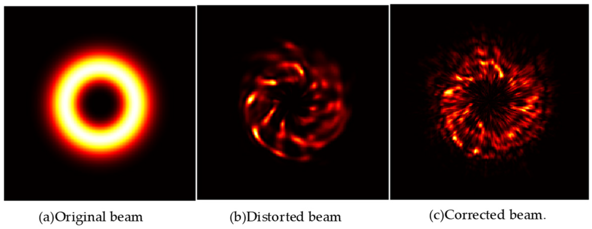
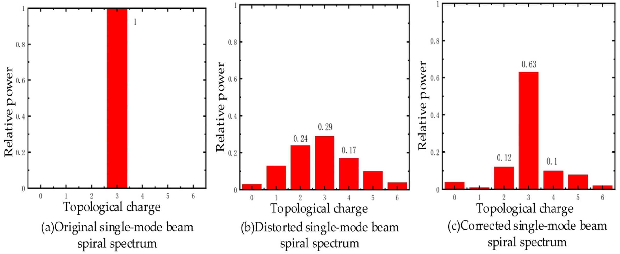
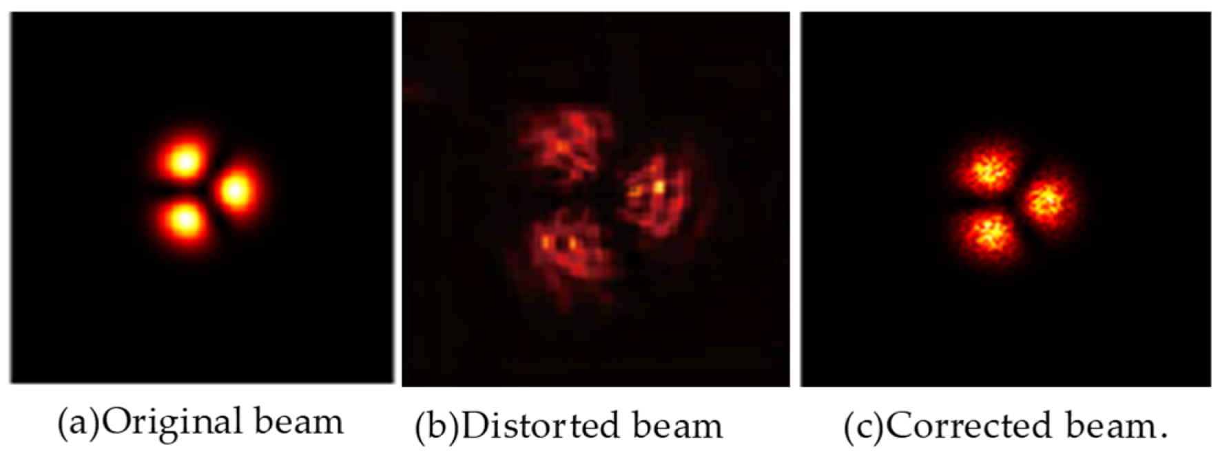
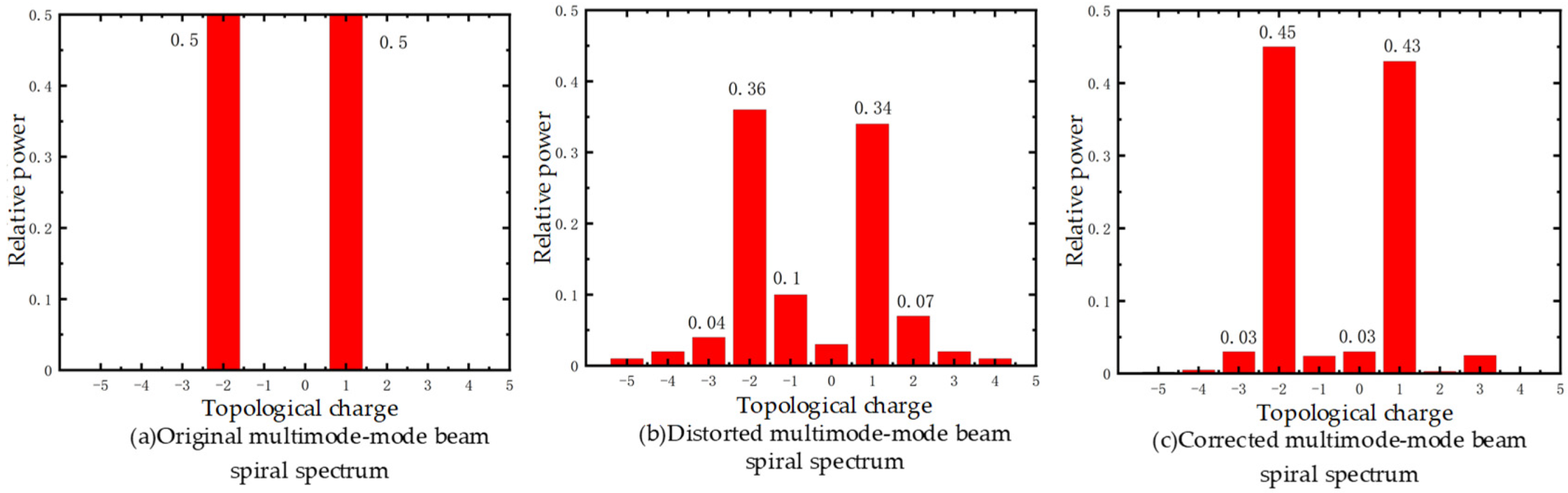
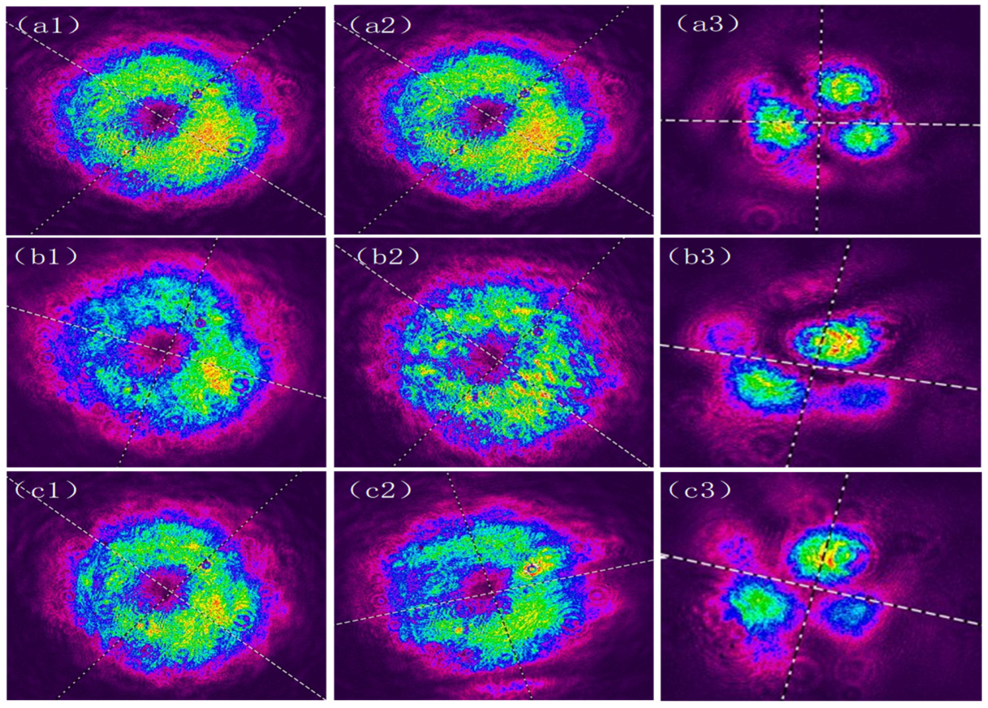
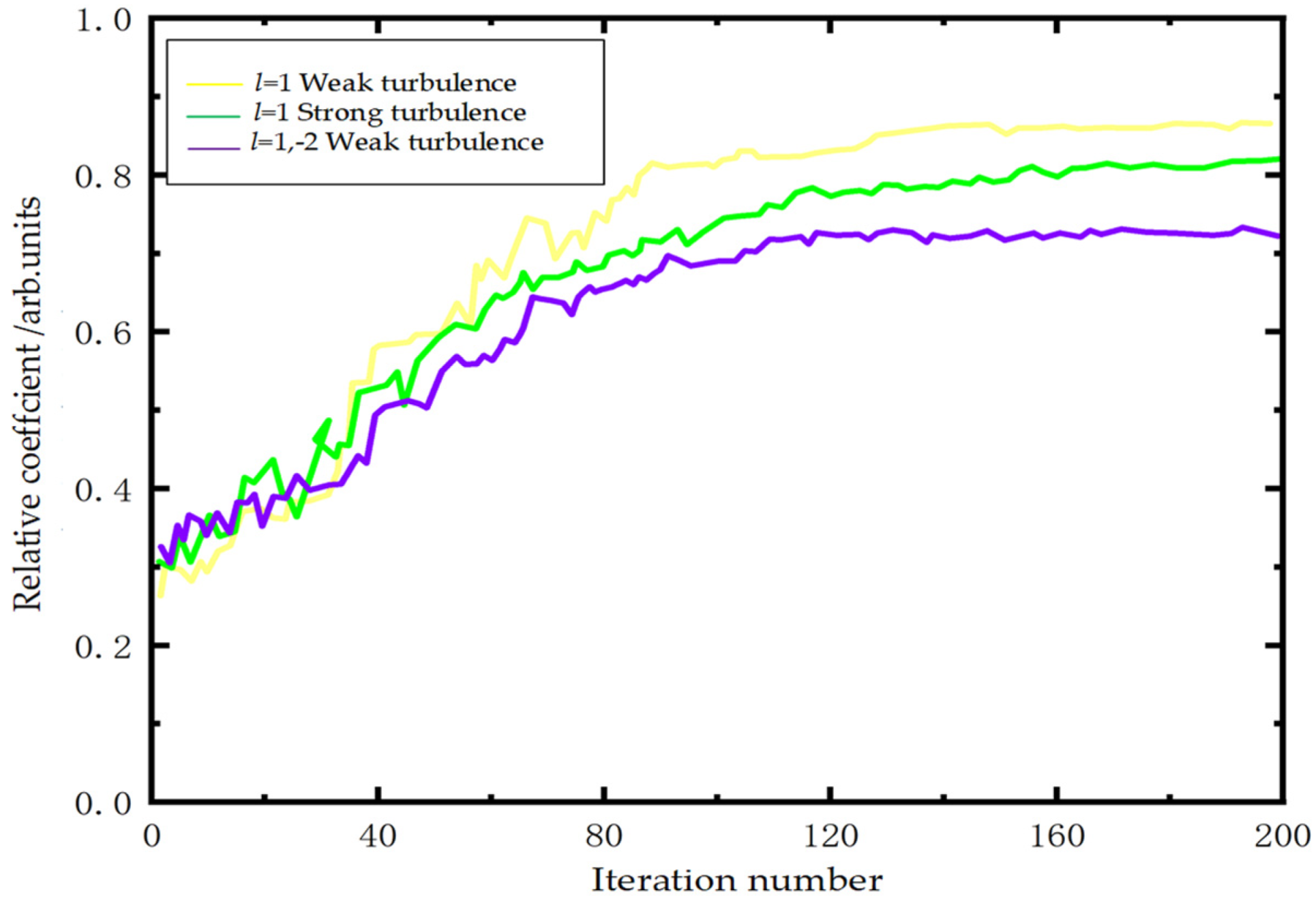
3.1. Simulation and Experimental Results

The parameters of the simulation experiment are selected as follows: beam waist radius ${\mathsf{\omega }}_0=3 \mathrm{c}$m, wavelength $\mathsf{\lambda }=632.8 \mathrm{n}$m, radial index p = 0, structure constant of atmospheric refractive index $C_n^2=1\times {10}^{-15}$m^−2/3 and $C_n^2=1\times {10}^{-13}$m^−2/3, and transmission distance z = 1 km. The number of iterations of the algorithm N = 200.

Figure 6 shows the variation curve of the intensity correlation coefficient of the topological load l = 3 before and after correction of the DDPG algorithm in weak turbulence. It can be seen from the figure that with the correction of the algorithm, the intensity correlation coefficient of the single-mode vortex beam can be increased from 0.58 to 0.88, indicating that the DDPG algorithm has high-quality correction performance.

Figure 7 shows the single-mode OAM beam with weak distortion before and after correction, based on the optimized DDPG algorithm. Figure 7b shows the intensity diagram of the single-mode LG beam after transmission in free space, and Figure 7c shows the intensity diagram of the single-mode LG beam after correction by the DDPG algorithm. It can be seen from the figure that the spot of the distorted single-mode vortex beam is broken and the energy is dispersed. The light spots corrected by the reinforcement learning DDPG algorithm show a relatively regular ring distribution, and the phase transition becomes clear and regular. A good correction effect is obtained. This shows that the DDPG algorithm can correct the intensity distribution of the single-mode OAM beam under distortion.

In order to verify that the DDPG algorithm also has the ability to improve the topological charge power, the spiral spectrum was also analyzed. Figure 8 shows the spiral spectrum power diagram of a single-mode OAM beam with topological charge l = 3 before and after correction by the DDPG algorithm under weak distortion. It can be seen from Figure 8b,c that the purity of the OAM mode after correction by the DDPG algorithm can be increased from 0.55 to 0.87, indicating that the DDPG algorithm also has an improving effect on mode purity under weak distortion.

To further illustrate the correction ability of the DDPG algorithm for single-mode vortex beams, the phase number of the intensity distribution of a single-mode beam under strong turbulence was analyzed. Figure 9 shows the curve of the phase number of the intensity distribution of a single-mode vortex beam under strong turbulence. From Figure 9, it can be seen that the phase number of the intensity distribution of the single-mode vortex beam was improved from 0.38 to 0.69 after correction by the algorithm, indicating that the DDPG algorithm has good correction performance for the intensity distribution under strong distortion.

Figure 10 shows a single-mode OAM beam under strong distortion pre- and post-intensity correction, based on the optimized deep deterministic policy gradient algorithm. Figure 10b shows the intensity of the single-mode LG beam after transmission in free space. From Figure 10c, it can be seen that the light spot changes from dispersion to a clear ring, but compared with the original single-mode beam, the corrected light intensity distribution is still poor in quality, and the strongest part of the light intensity is skewed to one side, which may be due to crosstalk between modes. It also shows that the deep deterministic policy gradient algorithm has a certain ability to correct the single-mode vortex beam under strong distortion.

The spiral spectrum can also be analyzed to verify the correction performance of the DDPG algorithm. Figure 11 shows the helical spectrum power diagram of a single-mode OAM beam with topological charge l = 3 before and after correction by the DDPG algorithm under strong distortion. It can be seen from Figure 11b,c that after correction by the deep deterministic policy gradient algorithm, the mode purity of a single-mode beam with topological charge l = 3 can be increased from 0.29 to 0.63. However, there is some crosstalk between the two modes. This shows that the deep deterministic policy gradient algorithm also has good correction performance for the single-mode OAM beam under strong distortion.

Figure 12 shows the variation curve of the intensity correlation coefficient of the topological charge l = −2, l = 1 spiral beam under weak turbulence. It can be seen from the figure that the intensity correlation coefficient of the multi-mode OAM beam can be increased from 0.66 to 0.96 with the correction of the DDPG algorithm, indicating that the deep deterministic policy gradient algorithm can greatly improve the intensity distribution quality of the multi-mode vortex beam.

Figure 13 shows the multi-mode multiplexed LG Beam with topological charge l = 2 and l = −1 under weak distortion before and after correction based on the optimized deep deterministic policy gradient algorithm. Figure 13b shows the intensity diagram of LG beam after transmission in free space. Figure 13c is the intensity diagram of the multi-mode LG beam after correction by the deep deterministic policy gradient algorithm. As can be seen from Figure 13b,c, the center intensity of each petal-shaped light intensity distribution after distortion and the light intensity distribution spot of the multi-mode vortex beam after distortion are broken and the energy is reduced. After correction by the deep deterministic policy gradient algorithm, relatively clear and obvious symmetrical light spots appear. A good correction effect is achieved. This shows that the deep deterministic policy gradient algorithm can correct the intensity distribution of the multi-mode multiplexed LG Beam under distortion.

From Figure 14b,c, it can be observed that the relative power of l = −2 reduces from 0.5 to 0.36 after distortion, and the relative power of l = 1 decreases from 0.5 to 0.34. After correction via the depth deterministic strategy gradient algorithm, the relative power of l = −2 ascends to 0.45, and the relative power of l = 1 rises to 0.43. The mode purity of the OAM beam in this mode is significantly enhanced, suggesting that the depth deterministic strategy gradient algorithm offers a relatively superior correction performance for multi-mode OAM beams under weak distortion.

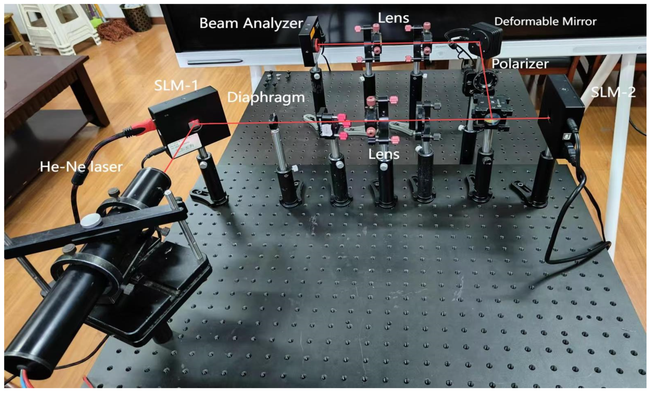
3.2. Experimental Research

The experimental scheme of the wavefront sensorless vortex light wavefront distortion adaptive correction system using the deep deterministic policy gradient algorithm is shown in Figure 15. In the experiment, a 632.8 nm He-Ne laser is used as the beam source, and the beam passes through the spatial light modulator (SLM) loaded with fork grating to generate single-mode or multi-mode vortex light. After the beam expansion and collimation of the two sets of lenses, the vortex beam is incident at SLM-2, which is loaded with the grayscale map simulating atmospheric turbulence. At this time, the vortex beam has wavefront distortion and is divided into two beams through the beam splitter mirror. One beam is an undistorted vortex beam that can be collected by the beam analyzer, and the other beam is a distorted vortex beam that is incident at the deformed mirror after collecting the distorted vortex data. Then, the corrected vortex beam reflected from the DM passes through the two sets of lenses into the beam analyzer, and the light intensity information is measured. The gradient algorithm of the depth deterministic strategy is used to calculate the deformation of the DM, and the closed-loop correction of the wavefront is achieved.

In this experiment, the corrector uses the ALPAO high-speed deformable mirror, produced in France, as shown in Figure 16:

Here are the main parameters of the deformable mirror used, as shown in

Table 1. The main parameters of the deformation mirror.

Driver Quantity	Diameter of the Mirror Surface (/mm)	Normalized Distance (/mm)	Maximum Deformation (/$\mu m$)	Stabilization Time (/$\mu m$)	Bandwidth (Hz)
69	10.5	1.5	60	800	>750

. From Table 1, it can be seen that the number of actuators in this deformable mirror is 69, the diameter of the mirror surface is 10.5 mm, the normalized distance between the actuators is 1.5 mm, the maximum deformation of the mirror surface is 60 µm, the time required for the deformable mirror to stabilize is about 800µs, and the bandwidth is greater than 750 Hz.

When the atmospheric structure constants are ${\mathrm{C}}_{\mathrm{n}}^2=1\times {10}^{-15}$m^−2/3 and ${\mathrm{C}}_{\mathrm{n}}^2=1\times {10}^{-13}$m^−2/3, the intensity distribution maps of different-order vortex beams before and after correction by a vortex beam analyzer are shown in Figure 17. Among them, Figure 17(a1–a3) shows the intensity distribution map of the vortex beam without turbulence and without correction in the experiment. In the experiment, due to manufacturing errors, surface roughness, uneven coating, and other factors of the optical components such as lenses, mirrors, and beam splitters in the optical system, as well as the characteristics of the beam analyzer used for measuring and displaying the intensity distribution, such as resolution, sensitivity non-uniformity, and response time, which affect the propagation of the beam and the intensity distribution measurement and display, even without turbulence, the intensity distribution non-uniformity problem will occur. Figure 17(b1–b3) shows the light intensity distribution after passing through turbulence, Figure 17(b1) shows the distorted single-mode vortex light under weak turbulence (l = 1), Figure 17(b2) shows the distorted single-mode vortex light under strong turbulence (l = 1), and Figure 17(b3) shows the distorted multi-mode vortex light under weak turbulence (l = 1, −2). Figure 17(c1–c3) shows the light intensity distribution after correction. After transmission through weak turbulence, the annular intensity distribution of the single-mode vortex light becomes distorted and deformed, and after passing through strong turbulence, the annular intensity becomes even more distorted. However, after correction, the intensity distribution becomes uniform, and the shape of the light spot also becomes regular. After transmission through turbulence, each petal-shaped light spot of the multi-mode multiplexed vortex light becomes distorted and deformed, but after correction, the petal-shaped light spots also become regular, and the intensity at the center of the petal-shaped light spots becomes stronger. Comparing Figure 7, Figure 10, Figure 13, and Figure 16, it can be seen that the experimental results for the changes in light intensity distribution before and after correction are consistent with the simulation results.

The variation in the light intensity correlation coefficient for single-mode vortex light (l = 1) and multi-mode multiplexed vortex light (l = 1, −2) with atmospheric structure constant $C_n^2=1\times {10}^{-15}$m^−2/3, as well as for single-mode vortex light (l = 1) with atmospheric structure constant $C_n^2=1\times {10}^{-13}$m^−2/3, is shown as a function of the number of iterations of the DDPG algorithm.

It can be seen from Figure 18 that after 200 iterations of the algorithm, the intensity correlation coefficient of single-mode vortex light can be improved from about 0.3 to about 0.85 in weak turbulence, from about 0.3 to 0.81 in strong turbulence, and from about 0.3 to about 0.72 in multi-mode multiplexed vortex light.

To verify the performance of DDPG in mode purity, the spiral spectrum of the vortex beam shown in Figure 17 was analyzed. As shown in Figure 19, where Figure 19(a1–a3) represents the spiral spectral distribution of the topological charge l = 1 single-mode vortex beam before and after correction in weak turbulence, Figure 19(a1) represents the initial vortex beam’s spiral spectral distribution before turbulence, Figure 19(a2) represents the spiral spectral distribution of the vortex beam after weak turbulence, and Figure 19(a3) represents the spiral spectral distribution of the vortex beam after correction by the DDPG algorithm. From Figure 19(a1–a3), we can see that the OAM mode purity after DDPG algorithm correction can be increased from 0.71 to 0.91. Figure 19(b1–b3) represents the spiral spectral distribution of the topological charge l = 1 single-mode vortex beam before and after correction in strong turbulence. From Figure 19(b1–b3), we can see that the OAM mode purity after DDPG algorithm correction can be increased from 0.48 to 0.85. Figure 19(c1–c3) represents the spiral spectral distribution of the topological charge l = 1,−2 multi-mode vortex beam before and after correction in weak turbulence. From Figure 19(c1–c3), we can see that the relative power of the OAM mode l = −2 is increased from 0.26 to 0.33, and the relative power of the OAM mode l = 1 is increased from 0.3 to 0.41 after DDPG algorithm correction. After analyzing Figure 19 and the simulation results in Figure 8, Figure 11, and Figure 14, the following conclusions were drawn.

4. Conclusions

In experiments on vortex light wavefront distortion correction without sensors, which apply phase recovery algorithms and SPGD algorithms, a spatial light modulator is generally adopted as the wavefront corrector. Before using the spatial light modulator as a corrector, a calibration experiment is necessary, to identify the relationship between the phase response of the spatial light modulator and the written grayscale values. Only then can the grayscale map calculated by the SPGD algorithm be loaded for wavefront correction. Nevertheless, the calibration experiment for the spatial light modulator is extremely complex and time-consuming, and it has high requirements regarding the parallelism and collimation of the light beam, which thereby increases the complexity and difficulty of implementing the wavefront distortion correction experiment. This paper proposes the use of the gradient algorithm from the DDPG combined with a classical adaptive optics system, employing a DM as the wavefront corrector for the system. There is no need for any preprocessing of the DM; it is only necessary to obtain the driving voltage of the DM when the optimal solution for the correlation coefficient of light intensity is achieved. Under the influence of the driving voltage, the DM alters the optical path of the incident light through its own mirror deformation, thereby accomplishing wavefront correction.

This paper presents a novel correction algorithm based on the DDPG algorithm for turbulence-induced wavefront aberration correction in helical beams. The proposed method can effectively correct wavefront aberration caused by atmospheric turbulence. The method has been validated through simulations and experiments for single-mode and multi-mode helical beam wavefront aberration correction, significantly improving the intensity correlation coefficient and mode purity. The proposed method has been proven to be effective in achieving wavefront aberration correction under different turbulence conditions. In the future, we will further study and optimize the DDPG algorithm to improve the correction performance of multi-mode helical beams in more complex turbulence conditions. We will also apply the proposed method to higher-order helical beams and test its performance and stability in real-world environments for use in free-space optical communication systems.

References

1. Liu, Z.; Fu, Y. The Design of a Novel Optical Communication Advance Margin Monitoring System. Chin. J. Sci. Instrum. 2006, 27, 689–690. [Google Scholar]
2. Liu, Y.; Gao, C.; Qi, X.; Weber, H. Orbital angular momentum(OAM)spectrum correction in free space optical communication. Opt. Express 2008, 16, 7091–7101. [Google Scholar] [CrossRef] [PubMed]
3. Li, M.; Takashima, Y.; Sun, X.; Yu, Z.; Cvijetic, M. Enhancement of channel capacity of OAM based FSO link by correction of distorted wavefront under strong turbulence. In Proceedings of the Frontiers in Optics 2014, Tucson, AZ, USA, 19–23 October 2014. [Google Scholar]
4. Duan, H.; Li, E.; Wang, H.; Yang, Z. The impact of mode orthogonality on wavefront measurement by Shack-Hartmann sensors. ACTA Opt. Sin. 2003, 23, 1143–1148. [Google Scholar]
5. Starikov, F.; Aksenov, V.; Atuchin, V.V.; Izmailov, I.V.; Kanev, F.Y.; Kochemasov, G.G.; Kudryashov, A.V.; Kulikov, S.M.; Malakhov, Y.I.; Manachinsky, A.N.; et al. Wave front sensing of an optical vortex and its correction in the close-loop adaptive system with bimorph mirror. In Proceedings of the Optics in Atmospheric Propagation and Adaptive Systems X, Florence, Italy, 17–20 September 2007. [Google Scholar]
6. Ke, X.; Zhang, D. Fuzzy control algorithm for adaptive optical systems. Appl. Opt. 2019, 58, 9967–9975. [Google Scholar] [CrossRef] [PubMed]
7. Poland, S.; Krstajić, N.; Knight, R.D.; Henderson, R.K.; Ameer-Beg, S.M. Development of a doubly weighted Gerchberg–Saxton algorithm for use in multi beam imaging applications. Opt. Lett. 2014, 39, 2431–2434. [Google Scholar] [CrossRef]
8. Jesacher, A.; Schwaighofer, A.; Fürhapter, S.; Maurer, C.; Bernet, S.; Ritsch-Marte, M. Wavefront correction of spatial light modulators using an optical vortex image. Opt. Express 2007, 15, 5801–5808. [Google Scholar] [CrossRef] [PubMed]
9. Baranek, M.; Behal, J.; Bouchal, Z. Optimal spiral phase modulation in Gerchberg-Saxton algorithm for wavefront reconstruction and correction. In Proceedings of the Thirteenth International Conference on Correlation Optics, Chernivtsi, Ukraine, 11–15 September 2017. [Google Scholar]
10. Vorontsov, M.A.; Sivokon, V.P. Stochastic parallel-gradient-descent technique for high-resolution wave-front phase-distortion correction. J. Opt. Soc. Am. 1998, 15, 2745–2758. [Google Scholar] [CrossRef]
11. Yang, H.; Li, X.; Jiang, W. High resolution imaging of phase-distorted extended object using SPGD algorithm and deformable mirror. In Proceedings of the Optical Design and Testing III (Part One of Two Parts), Beijing, China, 12–15 November 2007. [Google Scholar]
12. Ke, X.; Wang, X. Experimental Study on Helical Light Wavefront Deformation Correction. Acta Opt. Sin. 2018, 38, 204–210. [Google Scholar]
13. Ke, X.; Zhang, Y.; Zhang, Y.; Lei, S. Graphics Processor Acceleration of Wavefront Sensing-Free Adaptive Wavefront Correction System. Laser Optoelectron. Prog. 2019, 56, 88–96. [Google Scholar]
14. Jin, Y.; Zhang, Y.; Hu, L.; Huang, H.; Xu, Q.; Zhu, X.; Huang, L.; Zheng, Y.; Shen, H.L.; Gong, W.; et al. Machine learning guided rapid focusing with sensor-less aberration corrections. Opt. Express 2018, 26, 30162–30171. [Google Scholar] [CrossRef] [PubMed]
15. Ma, H.; Liu, H.; Qiao, Y.; Li, X.; Zhang, W. Numerical study of adaptive optics compensation based on convolutional neural networks. Opt. Commun. 2019, 433, 283–289. [Google Scholar] [CrossRef]
16. Gao, J.; Anantrasirichai, N.; Bull, D. Atmospheric turbulence removal using convolutional neural network. arXiv 2019, arXiv:1912.11350. [Google Scholar] [CrossRef]
17. Tian, Q.; Lu, C.; Liu, B.; Zhu, L.; Pan, X.; Zhang, Q.; Yang, L.; Tian, F.; Xin, X. DNN-based aberration correction in a wavefront sensorless adaptive optics system. Opt. Express 2019, 27, 10765–10776. [Google Scholar] [CrossRef] [PubMed]
18. Lillicrap, T.; Hunt, J.; Pritzel, A.; Hees, N.M.O.; Erez, T.; Tassa, Y.; Silver, D.; Wierstra, D. Continuous control with deep reinforcement learning. CoRR 2015, 71, 1059–1062. [Google Scholar]
19. Allen, L.; Beijersbergen, M.; Spreeuw, R.; Woerdman, J.P. Orbital angular momentum of light and the transformation of Laguerre-Gaussian laser modes. Phys. Rev. A 1992, 45, 8185f–8189. [Google Scholar] [CrossRef] [PubMed]
20. Zhang, W.; Ge, Y. Analysis of Vortex Shedding of Bridge Sections Based on the Modified Turbulent Freezing Hypothesis. J. Tongji Univ. 2008, 36, 1307–1313. [Google Scholar]
21. Wizinowich, P.; Acton, D.; Shelton, C.; Stomski, P.; Gathright, J.; Ho, K.; Lupton, W.; Tsubota, K.; Lai, O.; Max, C.; et al. First light adaptive optics images from the Keck II telescope: A new era of high angular resolution imagery. Publ. Astron. Soc. Pac. 2000, 112, 315–319. [Google Scholar] [CrossRef]
22. Pearson, J. Thermal blooming compensation with adaptive optics. Opt. Lett. 1978, 2, 7–9. [Google Scholar] [CrossRef] [PubMed]
23. Liu, T. Research on LQG Wavefront Control Technology in Adaptive Optics System; Xi’an University of Technology: Xi’an, China, 2023. [Google Scholar]
24. Freeman, R.; Pearson, J. Deformable mirrors for all seasons and reasons. Appl. Opt. 1982, 21, 580–588. [Google Scholar] [CrossRef] [PubMed]
25. Zhang, Z. Research on Fuzz Testing Technology Based on DDPG Reinforcement Learning Algorithm; Beijing University of Posts and Telecommunications: Beijing, China, 2021. [Google Scholar]
26. Sutton, R. Reinforcement Learning, 2nd ed.; Publishing House of Electronics Industry: Beijing, China, 2019. [Google Scholar]
27. Guo, X.; Fang, Y. Deep Reinforcement Learning: An Introduction to the Principles; Publishing House of Electronics Industry: Beijing, China, 2019. [Google Scholar]
28. Huang, H.; Ren, Y.; Yan, Y.; Ahmed, N.; Yue, Y.; Bozovich, A.; Erkmen, B.I.; Birnbaum, K.; Dolinar, S.; Tur, M.; et al. Phase-shift interference-based wavefront characterization for orbital angular momentum modes. Opt. Lett. 2013, 38, 2348–2350. [Google Scholar] [CrossRef] [PubMed]
Figure 1. Adaptive optics system correction schematic diagram.
Photonics 11 01116 g001
Figure 2. Schematic diagram of the deformation mirror correction principle.
Photonics 11 01116 g002
Figure 3. DDPG algorithm flowchart framework diagram.
Photonics 11 01116 g003
Figure 4. DDPG algorithm calibration schematic.
Photonics 11 01116 g004
Figure 5. DDPG algorithm correction vortex-beam-specific flowchart.
Photonics 11 01116 g005
Figure 6. The correlation coefficient of single-mode light intensity changes with the number of iterations under weak turbulence.
Photonics 11 01116 g006
Figure 7. The spot of the single-mode LG beam before and after correction with weak distortion.
Photonics 11 01116 g007
Figure 8. Spiral spectrum distribution diagram of a single-mode LG beam before and after correction under weak distortion.
Photonics 11 01116 g008
Figure 9. The correlation coefficient of single-mode light intensity changes with the number of iterations under strong turbulence.
Photonics 11 01116 g009
Figure 10. The spot of the single-mode LG beam before and after correction with strong distortion.
Photonics 11 01116 g010
Figure 11. Spiral spectrum distribution diagram of a single-mode LG beam before and after correction under strong distortion.
Photonics 11 01116 g011
Figure 12. The correlation coefficient of multi-mode light intensity changes with the number of iterations under weak turbulence.
Photonics 11 01116 g012
Figure 13. The spot diagrams of the multi-mode LG beam before and after correction under weak astigmatism.
Photonics 11 01116 g013
Figure 14. Spiral spectrum distribution diagram of a multi-mode LG beam before and after correction under weak distortion.
Photonics 11 01116 g014
Figure 15. Experimental set up.
Photonics 11 01116 g015
Figure 16. The physical map of deformation mirror.
Photonics 11 01116 g016
Figure 17. Distribution of light intensity in various order vortex beams before and after correction. (a1a3) Before turbulence; (b1b3) after turbulence; (c1c3) after correction.
Photonics 11 01116 g017
Figure 18. Correlation coefficient of light intensity with the number of iterations.
Photonics 11 01116 g018
Figure 19. The spiral spectral distribution maps of vortex beams of different orders before and after correction. (a1a3) The spiral spectral distribution maps of single-mode vortex beams with topological charge l = 1 before and after correction in weak turbulence. (b1b3) The spiral spectral distribution maps of single-mode vortex beams with topological charge l = 1 before and after correction in strong turbulence. (c1c3) The spiral spectral distribution maps of multi-mode vortex beams with topological charges l = 1,−2 before and after correction in weak turbulence.
Photonics 11 01116 g019