Automatic Compressive Sensing of Shack–Hartmann Sensors Based on the Vision Transformer

Abstract

Shack–Hartmann wavefront sensors (SHWFSs) are crucial for detecting distortions in adaptive optics systems, but the accuracy of wavefront reconstruction is often hampered by low guide star brightness or strong atmospheric turbulence. This study introduces a new method of using the Vision Transformer model to process image information from SHWFSs. Compared with previous traditional methods, this model can assign a weight value to each subaperture by considering the position and image information of each subaperture of this sensor, and it can process to obtain wavefront reconstruction results. Comparative evaluations using simulated SHWFS light intensity images and corresponding deformable mirror command vectors demonstrate the robustness and accuracy of the Vision Transformer under various guide star magnitudes and atmospheric conditions, compared to convolutional neural networks (CNNs), represented in this study by Residual Neural Network (ResNet), which are widely used by other scholars. Notably, normalization preprocessing significantly improves the CNN performance (improving Strehl ratio by up to 0.2 under low turbulence) while having a varied impact on the Vision Transformer, improving its performance under a low turbulence intensity and high brightness (Strehl ratio up to 0.8) but deteriorating under a high turbulence intensity and low brightness (Strehl ratio reduced to about 0.05). Overall, the Vision Transformer consistently outperforms CNN models across all tested conditions, enhancing the Strehl ratio by an average of 0.2 more than CNNs.

1. Introduction

Adaptive optics systems are widely used in ground-based telescopes [1,2], biological imaging [3], laser communications [4,5], human eye aberration correction [6], and other fields. In the field of astronomy, adaptive optics systems are effective technologies to resist atmospheric turbulence interference and make the angular resolution of ground-based telescopes close to or even reach the diffraction limit. Compared with space telescopes, adaptive optics systems provide a technology roadmap for ground-based telescopes to obtain high-quality star photos in a low-cost way. Almost all ground-based high-resolution imaging telescopes with apertures greater than 1 m have installed adaptive optics systems to correct the negative effects caused by atmospheric turbulence [7]. Owing to advancements in contemporary adaptive optics systems, the frontiers of ground-based optical and infrared astronomy are constantly being expanded [8]. In adaptive optics systems, Shack–Hartmann wavefront sensors (SHWFSs) are widely used because of their simple and easy-to-use structure, high utilization of light energy, and strong adaptability [9].

SHWFSs consist of a microlens array and a rear photoelectric sensor [10]. During the working process, SHWFSs sample the incident wavefront through a microlens array, and each sampled wavefront is assumed to be a planar wavefront. Then, the slope of each subaperture is calculated using the spot images obtained by the photoelectric sensor, and the incident wavefront is reconstructed using the modal [11,12] or zonal method [13,14].

In recent years, with the development of machine learning, deep learning algorithms have made significant breakthroughs in image recognition [15,16], natural language processing [17], and other fields. Therefore, deep learning algorithms have also been applied to the processing of data related to SHWFSs.

Z. Li and X. Li proposed a model based on fully connected neural networks, which converts the task of finding the centroid of the SHWFS subaperture into a classification task to resist external interference and improve the accuracy of the search [18]. In another study, Xu et al. also developed a model based on fully connected neural networks to convert the slopes of SHWFSs into corresponding Zernike coefficients [9]. Close et al. used U-net to convert the subaperture slopes of the SHWFSs to wavefront difference maps [19]. Similarly, DuBose et al. proposed a U-net-based model to eliminate the interference from non-uniform illumination and branch points in the phase distribution caused by atmospheric turbulence [20]. This model inputs the x slopes, y slopes, and total light intensity of each subaperture spot image of SHWFSs, directly outputting wavefront difference maps. These algorithms are non-end-to-end wavefront reconstruction methods that use the slopes of SHWFSs as input variables. However, for algorithms that calculate and reconstruct wavefront using the slopes of SHWFSs, the accuracy of these algorithms may be affected by the centroid positioning error and the averaged wavefront slope of SHWFSs [21]. Moreover, during the process of converting the subaperture spot image of SHWFSs into a slope, some pieces of information characterizing higher-order aberrations, which could be more effectively utilized, are lost [21].

In order to fully utilize the information of the subaperture spot images of SHWFSs, some researchers have developed end-to-end deep learning models that directly input complete SHWFS images. Hu et al. proposed an end-to-end U-net-based model that combines residual neural networks and can directly input images from SHWFSs and output reconstructed wavefront difference maps [21]. He et al. proposed another model to address the difficulty that SHWFSs face when capturing high-order aberrations with low subaperture counts. This model is based on convolutional neural networks to analyze individual subaperture spot images and a fully connected neural network to calculate the final Zernike coefficients [22]. Guo et al. and Hu et al. both utilized convolutional neural networks (CNNs) for the processing of light intensity images from SHWFSs. The former introduced a model that converts the light intensity image of SHWFSs directly into the corresponding Zernike coefficients [23]. The latter proposed another model that takes a downsampled light intensity image from SHWFSs as input and outputs Zernike coefficients ranging from the 2nd to the 120th terms [24].

As shown above, the underlying working model of the current deep learning algorithm for processing traditional SHWFSs is basically composed of a fully connected neural network, a convolutional neural network, and U-net. However, these deep learning models are not the best models for processing SHWFS data. The fully connected neural networks extract features layer-by-layer through fully connected layers, while the convolutional neural network and U-net extract features and produce results mainly through the convolution operation of the convolution kernel shared by all parts of the image in the convolution layer. The working principle of these models leads to the inability of the models to selectively process the data at different positions of the SHWFSs in the working process, while in the case of high turbulence intensity or low guide star brightness, the signal-to-noise ratio of some subaperture spot images in the SHWFSs decreases, and these low signal-to-noise ratio subaperture spot images often contaminate the final wavefront reconstruction results [10].

In addition, the data obtained by SHWFSs have sparsity, which makes it unnecessary for us to reconstruct the wavefront with all the subaperture spot image information. In order to fully utilize the sparsity of SHWFSs, some scholars have proposed sparse wavefront reconstruction algorithms specifically for SHWFSs. In 2014, Polans et al. first proposed a sparse wavefront reconstruction algorithm using Zernike polynomials to represent wavefront difference maps [25]. Then, Ke et al. proposed a similar algorithm [26]. The algorithms developed by these researchers use the Zernike coefficient as the basis function, and then they randomly select the slopes of the subapertures of the SHWFS and calculate the parameters of each Zernike coefficient through a recursive method. In their research, they found that we only need about ten percent of the subaperture spot image information of SHWFSs to reconstruct the entire wavefront. To reduce reconstruction error, a new basis function, which is called golden section sparse basis function, was proposed [27]. The majority of the previously discussed algorithms utilize a selection process applied to the subapertures of SHWFSs. However, these selections are all made randomly, and the repetitive nature of the iterations consequently contributes to an extended computational time for these algorithms. In 2021, Peng Jia et al. proposed an algorithm based on deep neural networks for compressive sensing wavefront reconstruction, which uses the signal-to-noise ratio of subaperture spot images as a selection criterion to filter out good subaperture information and uses CNNs to complete subaperture slope information and reconstruct phase difference maps [10]. This algorithm uses signal-to-noise ratio as the selection criterion and avoids the problem of long processing times caused by repeated iterations.

However, neural networks themselves have the ability to resist noise interference, so even low signal-to-noise ratio subaperture spot image information may still contain valuable information for reconstructing a wavefront. The method of directly discarding low signal-to-noise ratio subaperture spot image information in this algorithm is not appropriate. Moreover, beyond the spot image information of the subaperture, the position of the subaperture within the SHWFS holds significant value for wavefront reconstruction. This positional information can enhance the reconstruction accuracy, aiding in differentiating distortions that arise due to the physical location of subapertures within the sensor grid, such as the nonuniform illumination of the edge subapertures [28]. It can provide a more spatially accurate depiction of the wavefront distortions, allowing for a more precise correction. Despite these advantages, the positional information is not considered in all existing compressive sensing wavefront reconstruction algorithms for SHWFSs. The most important thing is that existing algorithms often need to compare the performance under various screening situations to determine the optimal screening method. However, the optimal subaperture selection method is influenced by various aspects such as the hardware structure of the SHWFS and specific situation of atmospheric turbulence, which makes it difficult for us to determine the optimal subaperture selection method.

Considering these difficulties, we introduce a novel algorithm that employs the self-attention mechanism of the Vision Transformer model [29] to automatically select the subapertures of SHWFSs. This innovative approach enables the Vision Transformer model to allocate weight values to each subaperture by taking into account both spot image information and the subaperture’s position information within the SHWFSs. In order to fully utilize the hardware resources of adaptive optical systems and avoid errors caused by the truncation of higher-order Zernike coefficients after using Zernike coefficients, we have the Vision Transformer model directly output the Deformable Mirror (DM) command vector.

For the first time, the Vision Transformer model is applied to SHWFS information processing. Simultaneously, we utilize a Residual Neural Network (ResNet) model [16], representing the CNN-based approach commonly employed in current scholarship [10,19,20,21,22,23,24,30]. To further extend our investigation, we train both the Vision Transformer and ResNet models under two scenarios: with and without data normalization. In doing so, we reassess the impact of normalization—a prevalent data preprocessing methodology—on the performance of these models. Normalization is a processing method that divides each pixel in the subaperture spot image of a SHWFS by the maximum pixel value of that spot image. Traditionally, normalization has been a common preprocessing method in CNN-based deep learning algorithms for SHWFSs because this preprocessing method can reduce the error caused by the non-uniformity of the spot intensity of each subaperture [23]. However, its effect on the performance of our proposed Vision Transformer model and the comparative ResNet model is a point of renewed investigation in this study.

The following sections of this article are as follows. In Section 2, we expound on the underlying principles of the Vision Transformer and ResNet models, elaborating on their specific hyperparameters. In Section 3, we delineate the methods employed for generating training and testing data and outline the processes involved in both training and testing, as well as the results obtained from these activities. In Section 4, we assess the corrective performance of the two models under two distinct data preprocessing approaches, differing primarily in the application of normalization. This evaluation considers aspects such as the residual phase difference, the energy distribution of the point spread function, and the performance of the models under varying R0 (Fried parameter, expressed in meters) values and guide star magnitudes. To mitigate the potential impact of model training randomness on the results and to test the algorithm’s repeatability, we trained ten models across four cases, subsequently illustrating the distribution of the model’s loss function. In Section 5, we summarize our findings and envisage future research directions.

2. Deep Learning Architectures and Principles

2.1. Detailed Exploration of ResNet

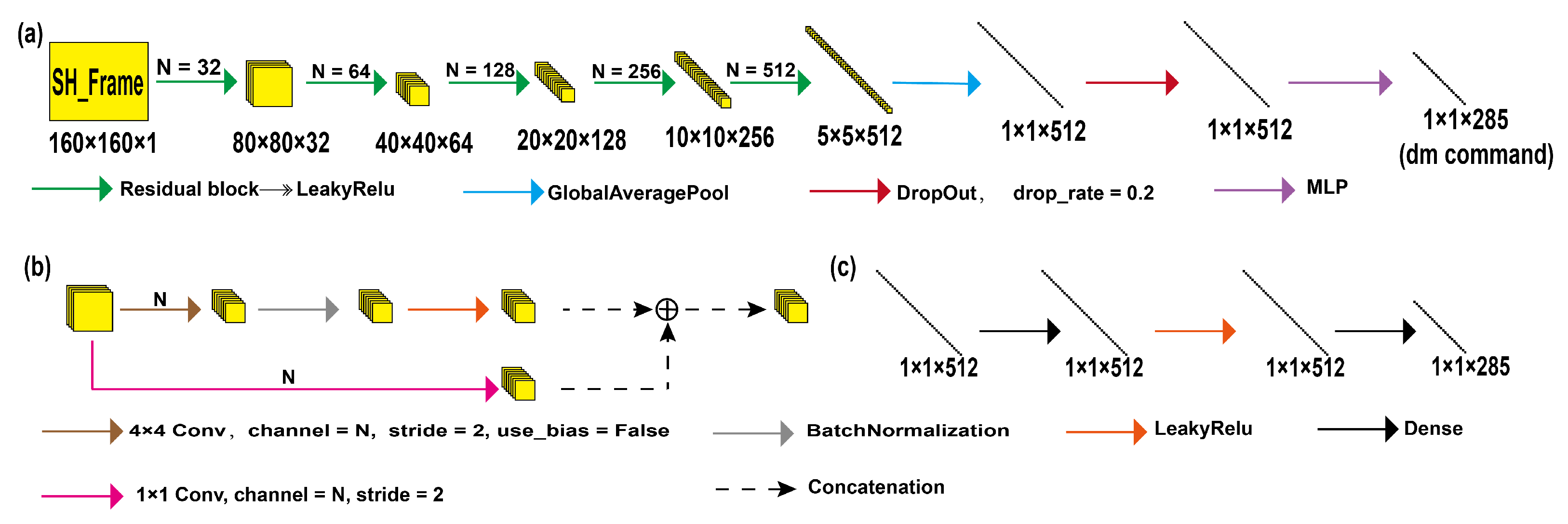
ResNet is a typical deep CNN, which has added residual connections to solve the problem of gradient vanishing and explosion caused by model deepening [16]. And Figure 1 is a diagram showing the structure of ResNet. In order to adapt to the size of the input data, we made appropriate modifications to this model and removed some layers of the neural network. The process begins with the input of the light intensity images from the SHWFS into the ResNet model. These images undergo the process of feature extraction by multilayer Residual Blocks. These blocks are essentially convolutional layers supplemented with residual connections, which facilitate the extraction of feature vectors pertinent to the light intensity image. To mitigate model overfitting, dropout layers are incorporated into the network for additional processing of these feature vectors. Ultimately, these feature vectors are passed through a fully connected layer that directly yields the final DM command vector.

2.2. Thorough Analysis of Vision Transformer

The Vision Transformer model, first proposed by Dosovitskiy et al. [29], provides a unique perspective on addressing computer vision problems. Unlike conventional methods that primarily leverage CNNs, the Vision Transformer model utilizes a Transformer architecture, a concept traditionally associated with natural language processing tasks.

In the Vision Transformer, images are segmented into numerous patches. And these image patches are then fed into the Transformer model, which allows for the capture of both local and global inter-patch relationships. A crucial component of the Transformer, the attention mechanism, enables the model to assign varying degrees of importance to different patches, focusing on information-rich areas.

This architecture has been shown to perform remarkably well, even surpassing traditional convolutional neural networks when applied to large-scale image datasets [29]. While the original application of the Vision Transformer was not in the field of SHWFS data processing, its design principle opens up new possibilities for innovative applications, such as those explored in our study.

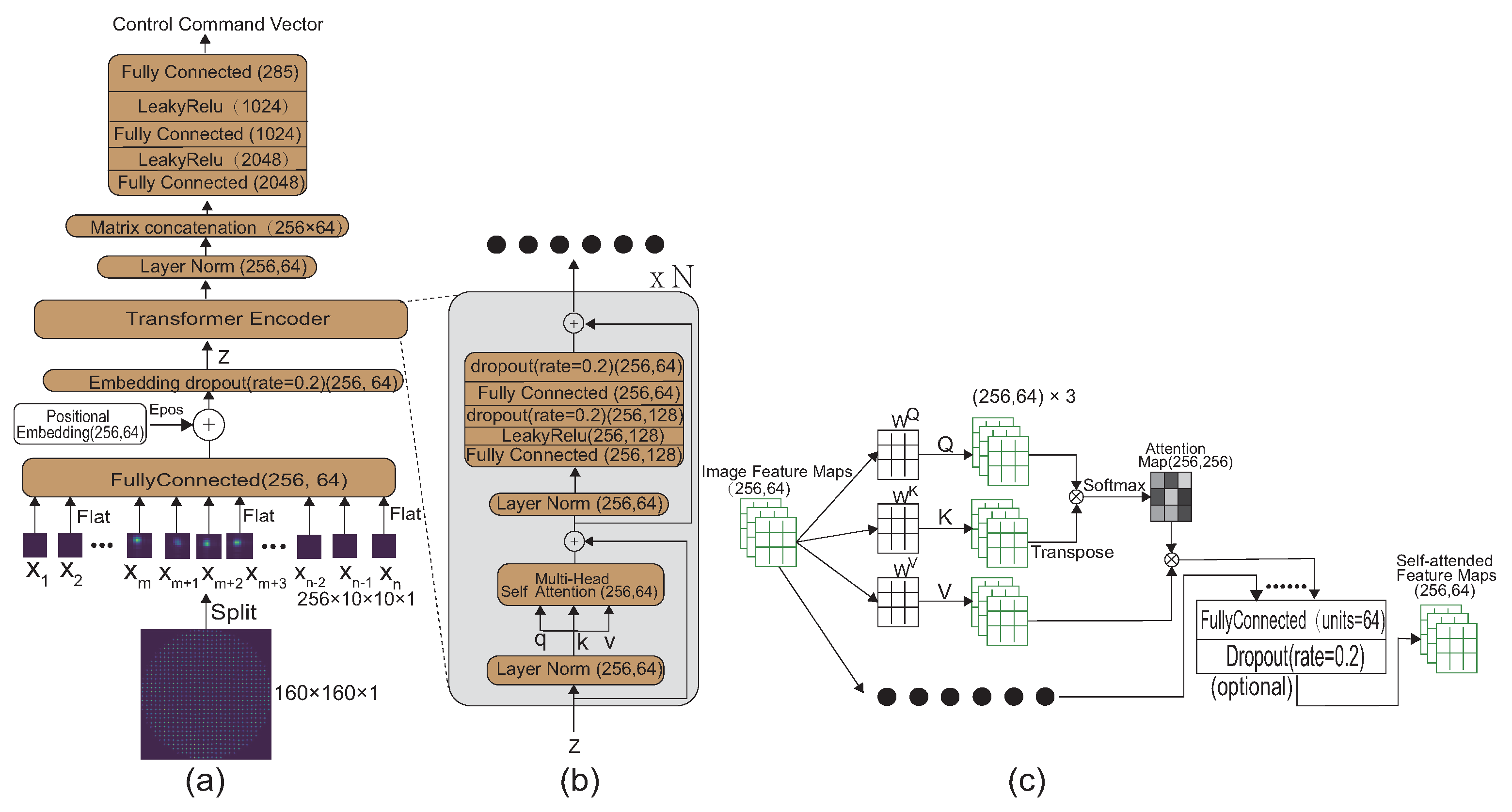
In our proposed algorithm, as shown in Figure 2a, each light intensity image from the SHWFS is segmented into a series of spot images following subaperture segmentation. Subsequently, each of these spot images is mapped into embedding vectors encapsulating spot image information via fully connected layers. These embedding vectors are then coupled with a series of one-dimensional vectors representing positional information. This results in a set of comprehensive embedding vectors, each embodying both image and positional information for individual subapertures within the SHWFS.

To mitigate potential overfitting during the training process, we employ a dropout layer with a dropout rate of 0.2 to refine the embedding vectors before passing them into the transformer encoder.

As shown in Figure 2b, the transformer encoder mainly consists of two parts, namely, the multi-head attention mechanism in the front and the multi-layer perceptron in the back. Each layer has residual connections to prevent gradient vanishing and exploding after the model deepens in the process of training.

The multi-head attention mechanism primarily comprises a layer normalization phase followed by a multi-head attention computation layer. While batch normalization [31], as used in ResNet [16], performs normalization across a set of features derived from light intensity images of varying guide star magnitudes and R0 values, layer normalization standardizes the embedding vectors of each subaperture of the SHWFS [32]. This normalization by subaperture stabilizes the layer inputs for subsequent computations, enabling more effective processing of the individualized subaperture information. The next multi-head attention mechanism, just as shown in Figure 2c, is represented by the following steps. The matrix of embedding vectors for all subapertures, denoted as $\mathit{Z}$, is transformed into query, key, and value matrices for each attention head:

$$\mathit{Q}=\mathit{Z}{\mathit{W}}_q$$

(1)

$$\mathit{K}=\mathit{Z}{\mathit{W}}_k$$

(2)

$$\mathit{V}=\mathit{Z}{\mathit{W}}_v$$

(3)

where $\mathit{Q}$, $\mathit{K}$, and $\mathit{V}$ are the query, key, and value matrices; $\mathit{Z}$ is the matrix of the input embedding vectors; and ${\mathit{W}}_q$, ${\mathit{W}}_k$, and ${\mathit{W}}_v$ are the weight matrices of the learnable linear transformations.

For each attention head, the attention scores between all pairs of subapertures are calculated using the scaled dot-product attention:

$$\mathit{A}=softmax\left({\displaystyle \frac{\mathit{Q}{\mathit{K}}^T}{\sqrt{d_k}}}\right)\mathit{V}$$

(4)

where $d_k$ is the dimension of the key vectors, $\mathit{A}$ is the output of a one-head attention value matrix, and the softmax function is applied along the rows. The result calculated by softmax is the Attention Map, which is the weight distribution of each subaperture of the SHWFS calculated by the Vision Transformer. By multiplying the Attention Map with the value matrix representing each subaperture information, we obtain the calculation result that assigns a certain weight value to each subaperture information.

Finally, if the number of attention heads is one and the dimension of the $\mathit{A}$ matrix is equal to the output dimension of the multi-head attention mechanism, we directly output the $\mathit{A}$ matrix as the output result of the multi-head attention mechanism. Otherwise, we concatenate all the $\mathit{A}$ matrices from all attention heads and use a fully connected layer and a dropout layer to calculate the final output result.

The subsequent multi-layer perceptron module, essentially a multilayer perceptron featuring residual connections, is tasked with further processing the obtained information.

These are the principles of the encoder in the Vision Transformer model. In practical applications, encoders often need to stack multiple layers to extract higher-order abstract features.

The information processed by the encoder, after undergoing a layer normalization process, is consolidated into a single vector. This vector is then input into a multi-layer perceptron for further processing to ultimately output a DM command vector.

In our Vision Transformer model, we set the number of heads in the multi-head attention mechanism to one, while the number of Transformer encoders is also configured to one to enhance real-time performance. With these configuration choices, we now proceed with a comparative analysis between the Vision Transformer and ResNet models to elucidate the performance advantages of our approach.

2.3. Comparative Examination of ResNet and Vision Transformer

In our study, we compare the performance of two neural network models, ResNet and Vision Transformer, in the context of processing light intensity images from SHWFSs. Both models exhibit robust capabilities in dealing with complex image-based tasks, but there are underlying differences in their working principles that render Vision Transformer more favorable in our specific use case.

ResNet functions chiefly by learning hierarchical features from images using convolutional layers. It employs the concept of residual connections to counteract the vanishing and exploding gradient problem that emerges in deeper networks, thereby substantially enhancing its performance across various visual tasks [16]. Nevertheless, when tasked with processing SHWFS light intensity images, ResNet’s shared convolutional kernel treats all regions of an image uniformly. This uniform treatment may not be optimal, considering the unique nature of SHWFS images: SHWFSs often experience low signal-to-noise ratios for certain subapertures due to low turbulence R0 and low guide star brightness, which can affect the final wavefront reconstruction results. The shared convolutional kernel approach of ResNet lacks the ability to distinguish and appropriately handle these subapertures, thus rendering it less efficient for this task, even though it is widely used in similar tasks.

In contrast, the Vision Transformer applies the principles of the Transformer architecture to vision-based tasks. This strategy introduces an attention mechanism, allowing the model to allocate diverse levels of focus to various parts of an image based on their significance. The Vision Transformer utilizes a multi-head attention mechanism to assign a specific weight value to each embedding vector, which encapsulates both corresponding subaperture spot image information and position information. This selective extraction of information and computation of the final result effectively mitigates the problem of low signal-to-noise ratios in subaperture spot images under conditions of a low R0 and low guide star brightness in SHWFSs. This approach ultimately enhances the robustness and accuracy of wavefront reconstruction results.

Therefore, the Vision Transformer model, with its unique approach to handling image data and its ability to focus adaptively on different parts of an image, presents a more tailored solution for our task of processing SHWFS light intensity images. However, theoretically speaking, the preprocessing operation of normalization can effectively reduce the error caused by the non-uniformity of spot intensity of each subaperture [23], thereby improving the performance of ResNet, which operates on the principle of feature extraction through convolution operations, while the preprocessing of normalization can normalize the pixel values of the subaperture spot image to a range of zero to one, which directly affects the calculation results of weight values in the multi-head attention mechanism in the Vision Transformer, so the impact of the normalization preprocessing on the performance of the Vision Transformer needs to be reevaluated.

3. Methodology

In order to compare the wavefront reconstruction capabilities of ResNet and the Vision Transformer under different guide star magnitudes and R0 conditions, we conducted numerical simulations based on an SCAO system. The specific configuration parameters of each module during the simulation process are shown in

Table 1. Principal parameters used with the Soapy SCAO simulation for artificial neural network (ANN) training and testing.

Module	Parameter	Value
Telescope	Diameter	8 m
	WFS Subapertures	16 × 16 (208 active)
	WFS Photon Noise	On
	DM Actuators	17 × 17 (4 redundant)
	NGS Wavelength	600 nm
	NGS Magnitude	u [8, 16) for training, [8, 9, …, 18] for testing while R0 was fixed to 0.20.
	R0	u [0.12, 0.18) for training, [0.05, 0.06, …, 0.20] for testing while magnitude was fixed to 8.
Science	Science Camera Wavelength	1650 nm

. The number of subapertures for the SHWFS is 16 × 16, with 208 active subapertures. The number of actuators for the deformable mirror is 17 × 17, with a total of 289 actuators. As four of them are located at the corners of the deformable mirror, they cannot affect the final correction result and are considered redundant actuators. Therefore, the length of the final DM command vector is 285. Throughout the simulation process, we used a point source at infinity as a natural guide with a wavelength of 600 nm, while the working wavelength of the CCD camera we used was set to 1650 nm.

3.1. Data Generation

We employed Soapy as our simulation tool for adaptive optics systems [33]. And the version of this tool used was 0.13.2. We opted for this tool due to its modularity, streamlining the construction of an adaptive optics system. To amass adequate data for deep learning model training, we utilized the Atmosphere (Atmos) module and the Wavefront Sensing (WFS) module to produce 70,000 light intensity images of SHWFS across eight guide star magnitudes with varying R0 values. These R0 values range uniformly from 0.12 (inclusive) to 0.18 (exclusive). Subsequently, a Reconstruction (Recon) module applied the computed slopes on these images, combined with the control matrix derived during calibration, to generate DM command vectors. We then adjusted the guide star magnitude of the primary light intensity image to fall uniformly between 8 (inclusive) and 16 (exclusive), as illustrated in Table 1, and introduced photon noise.

To assess the correction capabilities of the two deep learning models under varying guide star magnitudes and R0 scenarios, we replicated our method to produce a new set of light intensity images of SHWFS with differing turbulence strengths. For test data generation, we first standardized R0 at 0.2 and then successively adjusted the guide stars from magnitudes 8 through 18, securing 1000 light intensity images per magnitude. In a similar manner, with the guide star magnitude set at 8, we adjusted R0 in increments from 0.05 up to 0.20, acquiring 1000 light intensity images at each R0 value. These test data served to evaluate the correction efficiency of our deep learning models under various guide star magnitudes and R0 conditions.

3.2. Model Training and Testing

As shown in Figure 3, the 70,000 training data obtained in the previous step were first subjected to optional normalization preprocessing and then divided into a training set containing 60,000 data and a testing set containing 10,000 data. Based on these data, deep learning training was conducted. For our deep learning model training, we used a workstation equipped with NVIDIA Quadro P5000 GPU and 96 GB of memory. This workstation utilized a Conda virtual environment with Python 3.9 and TensorFlow 2.5.0 for training. During the training process, we set the batch size to 64, the learning rate to 0.01, and the loss function and metric function to Mean Absolute Error (MAE), and then we proceeded with subsequent training.

In the course of our training, we observed that the Adam optimization algorithm introduced significant instability. This likely stemmed from the model’s output being a DM command vector; heightened turbulence intensity might amplify the vector element values. Given Adam’s nature as a first-order gradient descent algorithm [34], this could precipitate a gradient explosion. To mitigate this risk, we opted for the SGD algorithm, which enhanced the stability of our neural networks’ training.

To mitigate potential stalls in performance improvement due to an excessive learning rate during training, we employed the “ReduceLROnPlateau” callback from the TensorFlow framework. This mechanism autonomously monitors the loss function value of the validation set, and if there is a decline of less than ${10}^{-4}$ for seven consecutive epochs, the learning rate is reduced to one-tenth of its current value. This allows the model to benefit from a smaller learning rate and enhances performance. The minimum threshold for the learning rate was set at ${10}^{-7}$. Furthermore, instead of using a predetermined number of epochs, which could risk suboptimal model performance or overfitting, we adopted the “EarlyStopping” callback. This halts the training process if the decline in the validation set’s loss function value over 10 consecutive epochs is below ${10}^{-6}$. After training, the model weights automatically reverted to the weight assignment that yielded the lowest validation loss. To address the potential variability in model performance across different configurations, we initially trained each configuration multiple times, selecting the model with the lowest MAE on the validation set under each configuration for subsequent analysis. Details and results for these chosen models are provided in

Table 2. Comparison of training times, epoch counts, and post-training loss function values of validation set for four distinct model configurations ¹.

Model Type	CNN with Nor	CNN Without Nor	Vision Transformer with Nor	Vision Transformer Without Nor
Training time	173.97 min	154.09 min	136.91 min	154.47 min
Training epoch	119	116	119	119
MAE value of validation set	0.6386	0.6792	0.52537	0.49808

¹ “nor” represents “normalization”.

. To further reduce the influence of training randomness, we increased the number of training times, leading to ten models per configuration. The outcome of these forty models are presented as a probability distribution in subsequent sections.

To assess the model’s performance under various turbulence intensities, we utilized the test dataset obtained from the prior step. Our testing infrastructure was a computer equipped with a Conda virtual environment running Python 3.7 and TensorFlow 2.9.1, backed by a Tesla k40c GPU and 31 GB of memory. Additionally, we evaluated the model’s inference speed for individual samples. For this, we shifted to a Conda virtual environment running Python 3.9 and TensorFlow 2.5.0. The resulting inference times were 3.363 ms for ResNet and 2.856 ms for the Vision Transformer.

Due to the fact that the ResNet algorithm itself is a type of CNN deep learning model, the ResNet algorithm we used here was to represent the widely used CNN deep learning model in the processing of light intensity image information of SHWFSs. Therefore, we use CNN to refer to ResNet in the following sections that showcase and discuss the results.

4. Assessing Model Correction Outcomes

4.1. Evaluation of Phase Correction Performance

Figure 4 provides a comparative analysis of the corrective capabilities of four distinct deep learning model configurations under varying R0 conditions. It is evident from the figure that the “CNN without normalization” exhibits the least effective correction among the three showcased R0 values. Conversely, “CNN with normalization” demonstrates a marked improvement over the former, yet still lags behind the two configurations of the Vision Transformer model. Among the Vision Transformer configurations, the “Vision Transformer without normalization” yields superior correction results compared to its normalized counterpart. Interestingly, as the R0 values rise, the disparity in correction performance between the “Vision Transformer without normalization” and “Vision Transformer with normalization” diminishes, transitioning from a difference of 0.1$\lambda$ in RMS values at R0 = 0.05 to merely 0.01$\lambda$ at R0 = 0.17. This indicates a shifting performance relationship between the two configurations as R0 increases.

Figure 5 provides a comparative evaluation of phase image corrections for atmospheric turbulence across varying guide star magnitudes. For both magnitudes 8 and 12, trends parallel to those observed in Figure 4 emerge: “CNN without normalization” underperforms, whereas “CNN with normalization” offers marginally better correction, albeit still substantially inferior to the Vision Transformer model. In contrast to the results in Figure 4, for a star magnitude of 8, the “Vision Transformer with normalization” surpasses the performance of its counterpart without normalization by a reduced RMS value difference of 0.02$\lambda$. Conversely, at a star magnitude of 12, the “Vision Transformer without normalization” stands out with the most effective correction. For a star magnitude of 16, while “CNN with normalization” outperforms “CNN without normalization” and “Vision Transformer without normalization” is superior to “Vision Transformer with normalization”, the overall performance of the Vision Transformer model lags behind that of the CNN model. But this may be due to the randomness of the sample.

Based on Figure 4 and Figure 5, we can conclude that for the processing tasks of light intensity images of SHWFSs under different R0 and guide star magnitudes, “CNN with normalization” has lower PV and RMS values compared to “CNN without normalization”, which also confirms the effectiveness of normalization preprocessing in improving CNN performance. For Vision Transformer, normalization preprocessing can actually improve the RMS value of the corrected phase image when the guide star brightness is low or R0 is small, while the opposite is true when the guide star brightness is high and R0 is large.

4.2. Analysis of Point Spread Function (PSF) Correction Results

Figure 6 presents the energy distribution curves of the PSFs after correction by models with four distinct configurations across various R0 conditions. To highlight the discrepancy between the model corrections and ideal outcome, we incorporate the energy distribution curve of a perfect PSF. Given that the range of R0 in Figure 6 spans a broader scope compared to Figure 4, we can more distinctly discern the trend of correction performance by the four deep learning configurations as R0 varies.

As illustrated in the subplot for R0 = 0.06, the intensity of atmospheric turbulence is high, resulting in Strehl ratios below 0.1 for all model configurations post-correction. Specifically, the “CNN with normalization” achieves a Strehl ratio of 0.022, slightly outperforming the 0.021 of the “CNN without normalization”. Consistent with previous findings, under such intense turbulence, the “ViT without normalization” emerges as the top performer with a Strehl ratio of 0.076, surpassing the 0.048 of the “ViT with normalization”. Notably, the Vision Transformer models consistently demonstrate superior performance over CNN models.

As R0 increases, indicating a decrease in turbulence intensity, the correction efficacy of all configurations improves progressively. While the relative performance rankings of the configurations remain consistent between R0 values of 0.06 to 0.16, the Vision Transformer models showcase a clear advantage over CNN models in terms of correction outcomes. Intriguingly, at R0 values of 0.18 and 0.20, the “ViT with normalization” outperforms its counterpart without normalization. This underscores the positive impact of normalization preprocessing on the Vision Transformer model in conditions of low turbulence intensity. Across the entire span of R0 values, Vision Transformer models consistently exhibit superior correction performance compared to CNN models.

In Figure 7, similar with Figure 6, energy distribution curves are depicted for models under four different configurations, where the variable is the star magnitude rather than R0. Figure 7 reveals that at a star magnitude of 9, the Strehl ratio for the “Vision Transformer with normalization” peaks at 0.824. This is followed by “Vision Transformer without normalization” at 0.795. The “CNN with normalization” achieves a Strehl ratio of 0.597, notably lower than the Vision Transformer models, even if it surpasses the 0.511 ratio of its counterpart without normalization. As the star magnitudes rise, the corrective capacities of all deep learning models wane. Notably, at a magnitude of 11, the “Vision Transformer without normalization” outperforms its normalized counterpart. However, while the Strehl ratios generally decline with increasing star magnitudes, the comparative performance order of the models remains consistent. To clarify, even when the star magnitude is equal to 17, the Strehl ratio of “CNN without normalization” is 0.108, slightly higher than the Strehl ratio of 0.106 for “CNN with normalization”, but this gap is very small, and this may be due to the randomness of the sample.

Figure 6 and Figure 7 compares and demonstrates the robustness of deep learning models with four distinct configurations while processing light intensity images from SHWFSs under different R0 values and star magnitudes. Similar to Figure 4 and Figure 5, the “Vision Transformer with normalization” model achieves a higher Strehl ratio compared to the “Vision Transformer without normalization” model when the guide star brightness is high or the turbulence intensity is low. However, when the guide star brightness is low or the turbulence intensity is strong, the “Vision Transformer without normalization” model can achieve a higher Strehl ratio. And in any case, the Vision Transformer model has a higher Strehl ratio than the widely used CNN model. At the same time, the Strehl ratio of correction results under different preprocessing conditions of the CNN once again proves the effectiveness of normalization preprocessing in improving the performance of CNN models.

Due to the fact that the above comparison shows only individual samples, it is susceptible to the randomness of the sample correction results. Therefore, in order to draw more convincing conclusions, we present the statistical trends observed in the correction outcomes of deep learning models across four specific configurations, considering varying R0 and star magnitudes.

4.3. Correction Comparison Across Models: R0 and Guide Star Magnitude Variations

To mitigate the effects of randomness from individual test samples on the final results, Figure 8 showcases the statistical outcomes of four differently configured models under varying guide star magnitudes and R0 conditions. Under different R0 scenarios, it is evident from the figure that as R0 increases, the performance of all four configurations continually improves. Specifically, when R0 is less than approximately 0.12, among the subfigures, the “Vision Transformer without normalization” model performs best, followed by the “Vision Transformer with normalization” and “CNN with normalization” models. The CNN model without normalization preprocessing exhibits the weakest performance. However, when R0 exceeds roughly 0.12, the “Vision Transformer with normalization” outperforms the “Vision Transformer without normalization” in terms of correction performance. Likewise, as guide star magnitudes change, the models exhibit consistent correction capabilities. The corrective capability of the “Vision Transformer without normalization” surpasses the “Vision Transformer with normalization” when the guide star magnitude is greater than around 11, making it the leading deep learning model. Surprisingly, the post-correction PV value of the “Vision Transformer with normalization” surpasses the optimal DM command vectors generated by Soapy under conditions of a guide star magnitude less than 10 and R0 greater than 0.12. This superior performance can likely be attributed to the robust generalization capabilities of the Vision Transformer model. Such capability enables it to discern intrinsic data features during training, subsequently applying these insights during inference, enhancing its correction performance across various conditions, including low turbulence intensities.

4.4. Loss Function Value Distributions Across Models

During the training process of a neural network, the initial weight value of the network, the optimization algorithm used, and the completeness and quality of the training data used for training all have a significant impact on the final performance of the network. Even if the same training data are used, the division of batches with the training data will directly affect the optimization direction of the neural network during training. Therefore, various factors lead to a certain degree of randomness in the final performance of the neural network after training. In order to weaken the impact of randomness during the training process on the comparison results and draw more representative conclusions, we trained 10 models for each model configuration, totaling 40 models. The probability distribution diagram of validation loss for these models is shown in Figure 9.

As illustrated in Figure 9, the mean and standard deviation of the MAE for “CNN with normalization” were 0.63114 and 0.00686, respectively. Compared with the MAE for “CNN without normalization”, both the mean and standard deviation decreased. Therefore, the probability distribution of the MAE values for those two kinds of models after multiple training, once again, proves the effectiveness of normalization preprocessing in improving the performance of the CNN model. Compared to the CNN, the performance of the Vision Transformer model is outstanding, and regardless of whether normalization is used, the performance of the model is significantly superior to that of the CNN model. Upon careful observation of the probability distributions of the two configurations of the Vision Transformer model, it can be seen that “Vision Transformer without normalization” has a lower mean and standard deviation, which is significantly better than “Vision Transformer with normalization”. In summary, from the results of the probability distribution map, “Vision Transformer without normalization” is better than “Vision Transformer with normalization”, and “CNN with normalization” is better than “CNN without normalization”.

It should be emphasized that the MAE values used here were obtained on the validation set, which contained training data with the same probability for different levels of guide brightness and turbulence intensities. Therefore, the results of this probability distribution map reveal the performance of the model under the condition that the probabilities of occurrence of various levels of guide brightness and turbulence intensities are equal. Therefore, the performance of the Vision Transformer model under specific levels of guide star brightness and turbulence intensities needs to refer to the previous figure.

5. Conclusions and Discussion

Our research demonstrates the innovative application of Vision Transformers to the analysis of SHWFS light intensity images, providing a robust alternative to traditional CNNs. Our evaluations reveal that Vision Transformers excel in accuracy and robustness under varied atmospheric and luminosity conditions, outperforming the commonly used CNNs, such as ResNet. The effectiveness of normalization preprocessing varies; it enhances CNN performance but has a mixed impact on Vision Transformers, enhancing them under conditions of low turbulence and high luminosity yet impairing their function in scenarios of high turbulence and low light levels. Despite these variations, the Vision Transformer maintains a consistent edge over CNNs in all conditions tested.

Vision Transformers distinguish themselves by employing a multi-head attention mechanism, which selectively processes subaperture information, optimizing the phase reconstruction by filtering detrimental inputs and enhancing beneficial ones. This advanced feature extraction method offers superior noise resistance, which is crucial under low light and high-turbulence conditions.

Traditionally favored for SHWFS light intensity image processing, CNNs leverage convolutional kernels for feature extraction, yet they struggle with the sparsity caused by atmospheric turbulence, especially under low guide star brightness and small R0 values. This limitation has prompted approaches like compressive sensing techniques. And the sparsity of atmospheric turbulence has also prompted deep-learning-based Peng Jia’s manual subaperture selection. But they are both facing the same challenging task of adapting to varying atmospheric and hardware conditions. In contrast, the Vision Transformer model, utilizing its multi-head attention mechanism, automatically adjusts weights to each subaperture, thereby enhancing the wavefront reconstruction’s accuracy and robustness without manual intervention. This capability not only underscores the model’s potential for SHWFS but also suggests its applicability to other sensors that also have a sparsity property, like pyramid wavefront sensors, and multi-sensor information fusion technology [35] within wide-field adaptive optics systems, which are promising areas for further exploration. And in order to verify the performance of the Vision Transformer model in practice, we will conduct relevant experiments to verify the actual performance of this algorithm.

References

1. Kim, D.; Choi, H.; Brendel, T.; Quach, H.; Esparza, M.; Kang, H.; Feng, Y.T.; Ashcraft, J.N.; Ke, X.; Wang, T.; et al. Advances in optical engineering for future telescopes. Opto-Electron. Adv. 2021, 4, 210040. [Google Scholar] [CrossRef]
2. Bian, Q.; Bo, Y.; Zuo, J.W.; Li, M.; Feng, L.; Wei, K.; Wang, R.T.; Li, H.Y.; Peng, Q.J.; Xu, Z.Y. First Implementation of Pulsed Sodium Guidestars Constellation for Large-aperture Multi-conjugate Adaptive Optics Telescopes. Publ. Astron. Soc. Pac. 2022, 134, 074502. [Google Scholar] [CrossRef]
3. Ji, N. Adaptive optical fluorescence microscopy. Nat. Methods 2017, 14, 374–380. [Google Scholar] [CrossRef] [PubMed]
4. Roberts, L.C.; Meeker, S.R.; Tesch, J.; Shelton, J.C.; Roberts, J.E.; Fregoso, S.F.; Troung, T.; Peng, M.; Matthews, K.; Herzog, H.; et al. Performance of the adaptive optics system for Laser Communications Relay Demonstration’s Ground Station 1. Appl. Opt. 2023, 62, G26–G36. [Google Scholar] [CrossRef]
5. Wright, M.W.; Morris, J.F.; Kovalik, J.M.; Andrews, K.S.; Abrahamson, M.J.; Biswas, A. Adaptive optics correction into single mode fiber for a low Earth orbiting space to ground optical communication link using the OPALS downlink. Opt. Express 2015, 23, 33705–33712. [Google Scholar] [CrossRef]
6. Liang, J.; Williams, D.R.; Miller, D.T. Supernormal vision and high-resolution retinal imaging through adaptive optics. J. Opt. Soc. Am. A 1997, 14, 2884–2892. [Google Scholar] [CrossRef] [PubMed]
7. Guo, Y.; Zhong, L.; Min, L.; Wang, J.; Wu, Y.; Chen, K.; Wei, K.; Rao, C. Adaptive optics based on machine learning: A review. Opto-Electron. Adv. 2022, 5, 200082. [Google Scholar] [CrossRef]
8. Swanson, R.; Lamb, M.; Correia, C.M.; Sivanandam, S.; Kutulakos, K. Closed loop predictive control of adaptive optics systems with convolutional neural networks. Mon. Not. R. Astron. Soc. 2021, 503, 2944–2954. [Google Scholar] [CrossRef]
9. Xu, Z.; Wang, S.; Zhao, M.; Zhao, W.; Dong, L.; He, X.; Yang, P.; Xu, B. Wavefront reconstruction of a Shack-Hartmann sensor with insufficient lenslets based on an extreme learning machine. Appl. Opt. 2020, 59, 4768–4774. [Google Scholar] [CrossRef]
10. Jia, P.; Ma, M.; Cai, D.; Wang, W.; Li, J.; Li, C. Compressive Shack-Hartmann wavefront sensor based on deep neural networks. Mon. Not. R. Astron. Soc. 2021, 503, 3194–3203. [Google Scholar] [CrossRef]
11. Wang, J.Y.; Silva, D.E. Wave-front interpretation with Zernike polynomials. Appl. Opt. 1980, 19, 1510–1518. [Google Scholar] [CrossRef]
12. Soloviev, O.; Vdovin, G. Hartmann-Shack test with random masks for modal wavefront reconstruction. Opt. Express 2005, 13, 9570–9584. [Google Scholar] [CrossRef] [PubMed]
13. Talmi, A.; Ribak, E.N. Wavefront reconstruction from its gradients. J. Opt. Soc. Am. A 2006, 23, 288–297. [Google Scholar] [CrossRef] [PubMed]
14. Fried, D.L. Least-square fitting a wave-front distortion estimate to an array of phase-difference measurements. J. Opt. Soc. Am. 1977, 67, 370–375. [Google Scholar] [CrossRef]
15. Krizhevsky, A.; Sutskever, I.; Hinton, G.E. ImageNet Classification with Deep Convolutional Neural Networks. In Proceedings of the Advances in Neural Information Processing Systems, Lake Tahoe, NV, USA, 3–6 December 2012; Pereira, F., Burges, C., Bottou, L., Weinberger, K., Eds.; Curran Associates, Inc.: Red Hook, NY, USA, 2012; Volume 25. [Google Scholar]
16. He, K.; Zhang, X.; Ren, S.; Sun, J. Deep Residual Learning for Image Recognition. In Proceedings of the 2016 IEEE Conference on Computer Vision and Pattern Recognition (CVPR), Las Vegas, NV, USA, 27–30 June 2016; pp. 770–778. [Google Scholar] [CrossRef]
17. Vaswani, A.; Shazeer, N.; Parmar, N.; Uszkoreit, J.; Jones, L.; Gomez, A.N.; Kaiser, L.u.; Polosukhin, I. Attention is All you Need. In Proceedings of the Advances in Neural Information Processing Systems, Long Beach, CA, USA, 4–9 December 2017; Guyon, I., Luxburg, U.V., Bengio, S., Wallach, H., Fergus, R., Vishwanathan, S., Garnett, R., Eds.; Curran Associates, Inc.: Red Hook, NY, USA, 2017; Volume 30. [Google Scholar]
18. Li, Z.; Li, X. Centroid computation for Shack-Hartmann wavefront sensor in extreme situations based on artificial neural networks. Opt. Express 2018, 26, 31675–31692. [Google Scholar] [CrossRef]
19. Swanson, R.; Lamb, M.; Correia, C.; Sivanandam, S.; Kutulakos, K. Wavefront reconstruction and prediction with convolutional neural networks. In Society of Photo-Optical Instrumentation Engineers (SPIE) Conference Series, Proceedings of the Adaptive Optics Systems VI, Austin, TX, USA, 10–15 June 2018; Close, L.M., Schreiber, L., Schmidt, D., Eds.; SPIE: Bellingham, WA, USA, 2018; Volume 10703, p. 107031F. [Google Scholar] [CrossRef]
20. DuBose, T.B.; Gardner, D.F.; Watnik, A.T. Intensity-enhanced deep network wavefront reconstruction in Shack-Hartmann sensors. Opt. Lett. 2020, 45, 1699–1702. [Google Scholar] [CrossRef] [PubMed]
21. Hu, L.; Hu, S.; Gong, W.; Si, K. Deep learning assisted Shack-Hartmann wavefront sensor for direct wavefront detection. Opt. Lett. 2020, 45, 3741–3744. [Google Scholar] [CrossRef]
22. He, Y.; Liu, Z.; Ning, Y.; Li, J.; Xu, X.; Jiang, Z. Deep learning wavefront sensing method for Shack-Hartmann sensors with sparse sub-apertures. Opt. Express 2021, 29, 17669–17682. [Google Scholar] [CrossRef]
23. Guo, Y.; Wu, Y.; Li, Y.; Rao, X.; Rao, C. Deep phase retrieval for astronomical Shack-Hartmann wavefront sensors. Mon. Not. R. Astron. Soc. 2022, 510, 4347–4354. [Google Scholar] [CrossRef]
24. Hu, L.; Hu, S.; Gong, W.; Si, K. Learning-based Shack-Hartmann wavefront sensor for high-order aberration detection. Opt. Express 2019, 27, 33504–33517. [Google Scholar] [CrossRef]
25. Polans, J.; McNabb, R.P.; Izatt, J.A.; Farsiu, S. Compressed wavefront sensing. Opt. Lett. 2014, 39, 1189–1192. [Google Scholar] [CrossRef] [PubMed]
26. Ke, X.; Wu, J.; Hao, J. Distorted wavefront reconstruction based on compressed sensing. Appl. Phys. B Lasers Opt. 2022, 128, 107. [Google Scholar] [CrossRef]
27. Juanjuan, L.; Dongmei, C.; Peng, J.; Can, L. Sparse decomposition of atmospheric turbulence wavefront gradient. Opto-Electron. Eng. 2018, 45, 170616. [Google Scholar]
28. Akondi, V.; Steven, S.; Dubra, A. Centroid error due to non-uniform lenslet illumination in the Shack-Hartmann wavefront sensor. Opt. Lett. 2019, 44, 4167. [Google Scholar] [CrossRef]
29. Dosovitskiy, A.; Beyer, L.; Kolesnikov, A.; Weissenborn, D.; Zhai, X.; Unterthiner, T.; Dehghani, M.; Minderer, M.; Heigold, G.; Gelly, S.; et al. An Image is Worth 16 × 16 Words: Transformers for Image Recognition at Scale. In Proceedings of the International Conference on Learning Representations, Virtual, 3–7 May 2021. [Google Scholar]
30. Suárez Gómez, S.L.; González-Gutiérrez, C.; Díez Alonso, E.; Santos Rodríguez, J.D.; Sánchez Rodríguez, M.L.; Carballido Landeira, J.; Basden, A.; Osborn, J. Improving Adaptive Optics Reconstructions with a Deep Learning Approach. In Proceedings of the Hybrid Artificial Intelligent Systems, Oviedo, Spain, 20–22 June 2018; de Cos Juez, F.J., Villar, J.R., de la Cal, E.A., Herrero, Á., Quintián, H., Sáez, J.A., Corchado, E., Eds.; Springer: Cham, Switzerland, 2018; pp. 74–83. [Google Scholar]
31. Ioffe, S.; Szegedy, C. Batch Normalization: Accelerating Deep Network Training by Reducing Internal Covariate Shift. In Proceedings of the 32nd International Conference on International Conference on Machine Learning, ICML ’15 PMLR, Lille, France, 6–11 July 2015; Volume 37, pp. 448–456. [Google Scholar]
32. Lei Ba, J.; Kiros, J.R.; Hinton, G.E. Layer Normalization. arXiv 2016, arXiv:1607.06450. [Google Scholar] [CrossRef]
33. Reeves, A. Soapy: An adaptive optics simulation written purely in Python for rapid concept development. In Society of Photo-Optical Instrumentation Engineers (SPIE) Conference Series, Proceedings of the Adaptive Optics Systems V, Edinburgh, UK, 26 June–1 July 2016; Marchetti, E., Close, L.M., Véran, J.P., Eds.; SPIE: Bellingham, WA, USA, 2016; Volume 9909, p. 99097F. [Google Scholar] [CrossRef]
34. Kingma, D.P.; Ba, J. Adam: A Method for Stochastic Optimization. In Proceedings of the 3rd International Conference on Learning Representations, ICLR 2015, Conference Track Proceedings, San Diego, CA, USA, 7–9 May 2015; Bengio, Y., LeCun, Y., Eds.; ICLR: San Diego, CA, USA, 2015. [Google Scholar]
35. Zhang, Y.; Gong, K.; Zhang, K.; Li, H.; Qiao, Y.; Ouyang, W.; Yue, X. Meta-Transformer: A Unified Framework for Multimodal Learning. arXiv 2023, arXiv:2307.10802. [Google Scholar] [CrossRef]
Figure 1. Overview of the Residual Neural Network (ResNet) model architecture employed for wavefront reconstruction from Shack–Hartmann wavefront sensor data. (a) Overall model structure: This panel shows the entire ResNet model where light intensity images from the Shack-Hartmann wavefront sensors (SHWFSs) are inputted. The model begins by processing these images through initial convolutional layers for downsampling, setting the stage for detailed feature extraction. (b) Feature extraction: Multilayer residual blocks refine the processed images into feature vectors. This stage emphasizes the extraction and enhancement of pertinent features necessary for accurate wavefront reconstruction. The “plus” symbol represents element-wise addition used to combine features from different layers. (c) Output generation: The feature vectors are fed into a multilayer perceptron, which processes the information to produce the final Deformable Mirror (DM) command vectors. This final stage is crucial for translating image-derived data into actionable corrections.
Photonics 11 00998 g001
Figure 2. The structure of the Vision Transformer model. The number in parentheses after the layer name indicates the size of the output vector for that layer. (a) depicts the overall structure of the model. To equip the Vision Transformer model with the capability to autonomously select subapertures of the SHWFS, the light intensity image is first segmented into a sequence of subaperture spot images. These are then mapped to a series of one-dimensional vectors via a fully connected layer, which are combined with position vectors to yield the final vectors that encapsulate both the image and position information of the subapertures. Following a dropout layer, these vectors proceed to the Vision Transformer’s encoder (b). The encoder utilizes its inherent multi-head attention mechanism (c) to automatically assign weight values to each subaperture-associated information, facilitating backpropagation. Subsequent to the layer normalization and matrix concatenation layers, the final DM command vectors are produced by the multiple fully connected layers.
Photonics 11 00998 g002
Figure 3. The training and testing process of deep learning models.
Photonics 11 00998 g003
Figure 4. Correction performance of deep learning models across four distinct configurations under varying R0 (Fried parameter, expressed in meters) conditions. Each column in this image from left to right is the phase image before correction, the phase image after “CNN with normalization” correction, the phase image after “CNN without normalization” correction, the phase image after “Vision Transformer with normalization” correction, and the phase image after “Vision Transformer without normalization” correction. In order to compare the differences before and after correction, each row of images shares the same color bar at the end of the row.
Photonics 11 00998 g004
Figure 5. Correction performance of deep learning models across four distinct configurations under varying guide star magnitude conditions. Each column in this image from left to right is the phase image before correction, the phase image after “CNN with normalization” correction, the phase image after “CNN without normalization” correction, the phase image after “Vision Transformer with normalization” correction, and the phase image after “Vision Transformer without normalization” correction. In order to compare the differences before and after correction, each row of images shares the same color bar at the end of the row.
Photonics 11 00998 g005
Figure 6. Energy distribution curves of point spread functions (PSFs) from different deep learning models for four configurations compared to ideal PSF distributions under varying R0 conditions. Sub-images illustrate the performance of various deep learning models under different configurations. In the legends, situated immediately beneath the figure title, “best psf”, “CNN with nor”, “CNN without nor”, “ViT with nor”, and “ViT without nor” correspond to “ideal psf”, “CNN with normalization”, “CNN without normalization”, “Vision Transformer with normalization”, and “Vision Transformer without normalization”, respectively. And the numbers in each sub-image denote the Zernike coefficients for each model type.
Photonics 11 00998 g006
Figure 7. Energy distribution curves of point spread functions (PSFs) from different deep learning models for four configurations compared to ideal PSF distribution under varying star magnitude conditions. Sub-images illustrate the performance of various deep learning models under different configurations. In the legends, situated immediately beneath the figure title, “best psf”, “CNN with nor”, “CNN without nor”, “ViT with nor”, and “ViT without nor” correspond to “ideal psf”, “CNN with normalization”, “CNN without normalization”, “Vision Transformer with normalization”, and “Vision Transformer without normalization”, respectively. And the numbers in each sub-image denote the Zernike coefficients for each model type.
Photonics 11 00998 g007
Figure 8. Comparison of correction performance for four configurations of deep learning models across varying R0 values and guide star magnitudes. In the legend at the top of the figure, “CNN with nor”, “CNN without nor”, “ViT with nor”, and “ViT without nor” correspond to models “CNN with normalization”, “CNN without normalization”, “Vision Transformer with normalization”, and “Vision Transformer without normalization”, respectively. And “test label” denotes the optimal DM command vector generated by Soapy. The sub-images in the first column display the Strehl ratio on a linear vertical scale, while the second and third columns show RMS and PV metrics on a logarithmic scale. And the error bar in the line graph refers to the standard deviation of the test data in the case of R0 or magnitude, while the curve refers to the average values.
Photonics 11 00998 g008
Figure 9. The probability distribution map showcasing the mean absolute error (MAE) values obtained on the validation set after training the model under four distinct configurations.
Photonics 11 00998 g009