Underwater Dynamic Polarization-Difference Imaging with Greater Applicability

Abstract

Available polarization-difference imaging techniques face serious challenges in imaging speed and application range. To address these issues, this paper proposes an underwater dynamic polarization-difference imaging method with greater applicability. First, the intensity distribution of backscattered light is estimated via the Stokes vector. Afterward, the differential operation between the total intensity of light and the amplified estimation result of backscattered light makes clear imaging immediately accessible. Regardless of the movement states and polarization characteristics of the target, experimental results consistently demonstrate that the backscattered light can be eliminated to a great extent, and imaging quality and applicability are significantly enhanced. Meanwhile, the proposed method is immune to unexpected factors such as uneven illumination and has good stability. More importantly, there are also apparent advantages in terms of imaging time.

1. Introduction

Underwater optical imaging has broad application prospects in many fields such as underwater rescue, seabed resource exploration, submarine vehicle observation, etc. [1]. However, absorption and scattering cause serious degradation of imaging quality, which severely limits its usefulness in practical scenarios [2]. In response to this challenge, various methods have been proposed to improve imaging clarity, leading to a proliferation of techniques such as synchronous scanning imaging [3], range-gated imaging [4], indirect time-of-flight imaging [5], deep learning [6,7], etc. Leveraging the partially polarized properties of the backscattered light [8], polarization imaging has also registered a superior descattering performance. Coupled with its simple operation and low cost, this has elevated it to be a research hotspot [9,10,11,12,13].

Among polarization-based imaging techniques, polarization-difference imaging (PDI) is a highly regarded tool. Cameron et al. established a solid theoretical foundation for this technology based on the double cones of many invertebrates and vertebrates [14]. Thus, it was not long before polarization-difference imaging, inspired by some biological visual systems, was proposed by Rowe et al. [15]. This research quickly gained widespread attention and has grown significantly as a result. Tyo et al. exploited PDI to enhance the point-spread function [16]. Walker et al. conducted research on polarization subtraction imaging [17]. Zhu et al. presented the polarization-based range-gated imaging method, suppressing the backscattered light in dimensions of both time and polarization [18]. Shi et al. proposed the means of polarization difference ghost imaging, again realizing the strengths of both techniques [19]. In pursuit of imaging clarity, the researchers did not neglect other meaningful issues. Considering the imaging speed, Guan and Tian utilized the Stokes vector to enhance PDI, facilitating the generation of two novel methods targeting imaging timeliness [20,21]. Hu et al. implemented illumination modulation via the Mueller matrix, increasing the effects of incident polarized light on imaging quality [22]. To overcome the barriers of inconsistent polarization direction, Wang et al. proposed a new method based on periodic integration, obtaining better performance in detail enhancement and noise suppression [23].

Even though significant progress has been made, two issues warrant further consideration. The imaging speed remains a limitation, as many existing methods, including Guan’s and Tian’s methods, are oriented towards imaging static targets, potentially hindering their applicability in dynamic scenarios. On the other hand, the difference process may inevitably eliminate signals from targets with strong depolarization abilities, resulting in a somewhat homogeneous range of applicable target types. This underscores the urgent need for in-depth research to develop new methods capable of effectively imaging moving targets with various polarization characteristics, thereby driving the continuous advancement of imaging techniques.

In this paper, to enhance the dynamic performance and applicability of underwater polarization-difference imaging, a computational difference method based on the Stokes vector [S₀ S₁ S₂]^T is proposed. By exploiting the low-pass filtering in the frequency domain, the possible target signal in S₁ is eliminated, ensuring the estimation of the intensity distribution of the backscattered light. Subsequently, the clear imaging result is generated via the differential operation between S₀ and the magnified estimation result. Static and dynamic imaging experiments on targets with single or complex polarization characteristics were conducted. The results indicated that even in the presence of interfering factors such as uneven illumination, target jitter, and so on, the backscattered light can always be effectively eliminated. Meanwhile, the processing time meets the requirements of dynamic imaging. All this proves that prominent descattering effects, real-time characteristics, greater applicability, and good stability can be obtained simultaneously, meaning that there is huge potential for practical application.

2. Methodology of Underwater Dynamic Polarization-Difference Imaging

According to [15], the definition of PDI is as follows:

$$I_{pd}(x,y)=I_{\parallel }(x,y)-I_{\perp }(x,y).$$

(1)

Here, I_pd(x,y) is the result of polarization-difference imaging, and $\parallel$ and $\perp$ denote two orthogonal linear polarizations.

Usually, the acquisition of two orthogonally polarized images is accomplished by rotating the polarizer. This avenue not only necessitates determining the orientation of the polarizer, but is also time-consuming. To streamline this process, the Stokes vector is chosen as the input image instead. As the complete description of polarization states, the Stokes vector is defined as follows:

$$\begin{array}{l}{S}_0=I_0+I_{90}=T_0+B_0+T_{90}+B_{90},\\ S_1=I_0-I_{90}=T_0+B_0-T_{90}-B_{90},\\ S_2=I_{45}-I_{135}=T_{45}+B_{45}-T_{135}-B_{135}.\end{array}$$

(2)

Since the circularly polarized component accounts for a small proportion, only the first three components are given. Taking the incident light as a reference, I₀, I₄₅, I₉₀, and I₁₃₅ denote the polarized image at the corresponding angles, respectively. These images can be decomposed into two parts, with one created from the target light T, i.e., the desired clear imaging result. The undesired backscattered light B forms the other part, which is the object to be eliminated by PDI. Further, according to polarization characteristics, both T and B can be subdivided into two parts. Under these circumstances, four polarized sub-images can be represented as follows [24].

$$I_0=T_p{\cos }^2\theta +{\displaystyle \frac{1}{2}}{T}_n+B_p{\cos }^2\phi +{\displaystyle \frac{1}{2}}{B}_n,$$

(3)

$$I_{45}=T_p{\cos }^2(\theta -45)+{\displaystyle \frac{1}{2}}{T}_n+B_p{\cos }^2(\phi -45)+{\displaystyle \frac{1}{2}}{B}_n,$$

(4)

$$I_{90}=T_p{\sin }^2\theta +{\displaystyle \frac{1}{2}}{T}_n+B_p{\sin }^2\phi +{\displaystyle \frac{1}{2}}{B}_n,$$

(5)

$$I_{135}=T_p{\sin }^2(\theta -45)+{\displaystyle \frac{1}{2}}{T}_n+B_p{\sin }^2(\phi -45)+{\displaystyle \frac{1}{2}}{B}_n.$$

(6)

The subscripts p and n represent the polarized and unpolarized components separately. The former has non-zero intensity only in the direction of polarization, while the latter exhibits equal intensity in any direction [8]. θ and φ indicate the angle of polarization (AOP) of the target and the backscattered light, respectively. By substituting Equation (3) into Equation (2), the Stokes vector [S₀ S₁ S₂]^T can be calculated with a quaternion system.

$$\left[\begin{array}{l}{S}_0\\ S_1\\ S_2\\ 0\end{array}\right]=\left[\begin{array}{cccc}{\cos }^2\theta +{\sin }^2\theta & {\displaystyle \frac{1}{2}}+{\displaystyle \frac{1}{2}}& {\cos }^2\phi +{\sin }^2\phi & {\displaystyle \frac{1}{2}}+{\displaystyle \frac{1}{2}}\\ {\cos }^2\theta -{\sin }^2\theta & {\displaystyle \frac{1}{2}}-{\displaystyle \frac{1}{2}}& {\cos }^2\phi -{\sin }^2\phi & {\displaystyle \frac{1}{2}}-{\displaystyle \frac{1}{2}}\\ {\cos }^2(\theta +{45}^{\circ })-{\sin }^2(\theta +{45}^{\circ })& {\displaystyle \frac{1}{2}}-{\displaystyle \frac{1}{2}}& {\cos }^2(\phi +{45}^{\circ })-{\sin }^2(\phi +{45}^{\circ })& {\displaystyle \frac{1}{2}}-{\displaystyle \frac{1}{2}}\\ 0& 0& 0& 0\end{array}\right]\left[\begin{array}{l}{T}_p\\ T_n\\ B_p\\ B_n\end{array}\right]$$

(7)

Only the intermediate process is presented, to highlight the effect of the addition and subtraction operations therein on the polarized and unpolarized components. As can be seen, S₀ indicates the total light intensity, encompassing all polarized and unpolarized components. Since S₁ and S₂ are the results of image subtraction, the unpolarized components are eliminated, leaving only the polarized components. Consequently, the Stokes vector is as follows:

$$\begin{array}{l}{S}_0=T_p+T_n+B_p+B_n,\\ S_1=T_p\cos 2\theta +B_p\cos 2\phi ,\\ S_2=T_p\sin 2\theta +B_p\sin 2\phi .\end{array}$$

(8)

Fortunately, T_p can also be eliminated depending on the polarization properties of the target. As a result, it is possible to estimate the intensity distribution of the backscattered light via S₁ and S₂. Then, the differential operation between S₀ and the estimation result makes clear imaging available immediately.

Considering the polarization characteristics of T, one class of targets has strong depolarization abilities, leading to the intensity of T_p being 0. For this reason, the target light does not contribute to S₁ and S₂. In addition, the absence of polarized components causes the target signal to be eliminated in the differential process, making it impossible for previous PDI methods to handle such targets. For highly polarized targets, the intensity of T_p is substantial. From the imaging results in [25], it is easy to infer that θ is 0°. Hence, T_p is preserved only in the differential process of S₁, while during the formation of S₂, the target signal is again eliminated in its entirety. It should be noted that the remaining target light in S₁ may create obstacles in intensity estimation. However, it is a prerequisite for existing PDI techniques to work well.

As shown in the above analysis, regardless of the polarization characteristics of the target, S₂ is able to directly serve as the estimation result for the intensity distribution of B_p, as follows:

$$S_2(B)=S_2=B_p\sin 2\phi ,$$

(9)

where S₂(B) indicates the intensity distribution of backscattered light. For lowly polarized targets, S₁ is also able to directly serve as the estimation result for the intensity distribution of B_p, as follows:

$$S_1(B)=S_1=B_p\cos 2\phi .$$

(10)

As for the possible hindrance from the highly polarized target in S₁, it can be removed by the low-pass filtering method [26].

$$S_1(B)=F{T}^{-1}[FT(S_1)\times H(u,v)]=B_p\cos 2\phi .$$

(11)

Here, FT and FT⁻¹ are the Fourier transform and inverse transform, and H(u,v) represents the low-pass filter in the frequency domain. According to [27], the Gaussian low-pass filter is chosen for its smoothing properties.

Hence, for lowly and highly polarized targets, the estimation result of B_p can be represented as follows:

$$B_p=\sqrt{S_1^2(B)+S_2^2(B)}.$$

(12)

Hence, it seems that the low-pass filter needs to be employed again for the determination of B_n. Fortunately, there is a simpler and more direct avenue. As per the definition of the degree of polarization (DOP) [24], there is a link between B_p and total intensity, i.e., the following:

$$P_{scat}={\displaystyle \frac{B_p}{B_{total}}}={\displaystyle \frac{B_p}{B_p+B_n}}.$$

(13)

where P_scat denotes the DOP of backscattered light and B_total is the total intensity of backscattered light. From Equation (13), without estimating B_n, B_total can be obtained directly by amplifying B_p as follows:

$$B_{total}={\displaystyle \frac{1}{P_{scat}}}{B}_p=\alpha ·B_p.$$

(14)

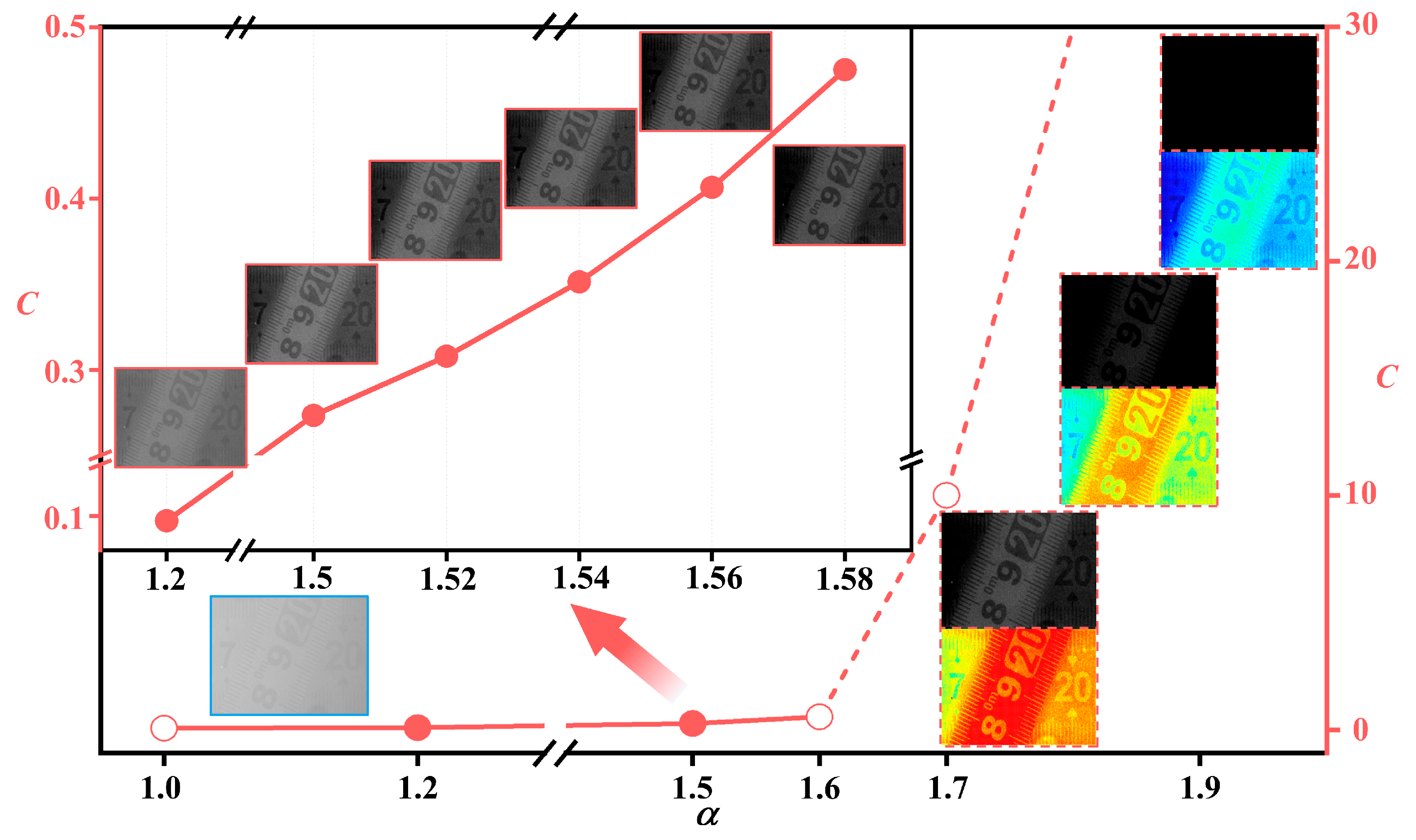
Because P_scat is an unknown parameter and, for simplicity, the proportional factor (α) is used to represent amplification, α has physical significance as the reciprocal of P_scat. Estimation for this parameter can be found in Section 4.

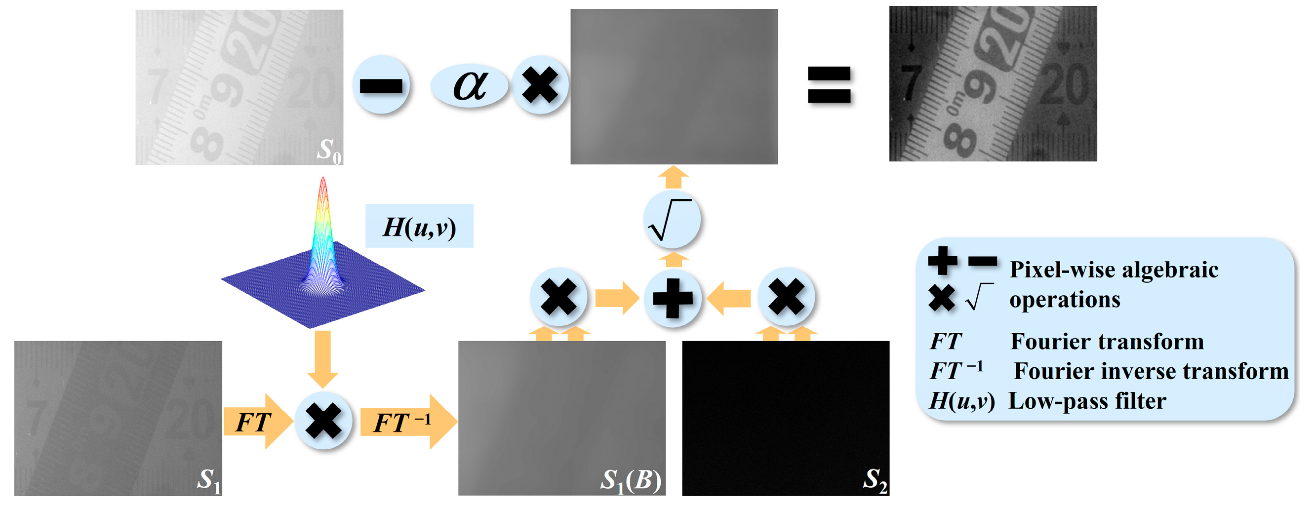
Therefore, the differential operation between S₀ and amplified B_p could be an effective way to eliminate the backscattered light, i.e., the following:

$$T=S_0-\alpha \sqrt{S_1^2(B)+S_2^2(B)}.$$

(15)

This is our dynamic polarization-difference imaging method based on the Stokes vector, in which α represents the proportional factor. The processing flow is shown in Figure 1. Here, a composite target is used as an example. The ruler below is made of steel, and light predominantly reflects specularly off its surface, making it a highly polarized target. The ruler above is made of plastic and the light is diffusely reflected mainly from its surface, making it a lowly polarized target. In this way, this composite target has complex polarization characteristics.

As can be seen, the proposed method accomplishes PDI via the differential computation between the total intensity and the estimation result of the backscattered light. As the spatial variation of the backscattered light is involved, instances of of inhomogeneous intensity distribution can be well countered. Meanwhile, this approach applies to targets with either single or complex polarization characteristics, which allows for greater applicability. In addition, the priors such as the background region can be avoided, making our method capable of dynamic imaging. Based on these facts, it can be anticipated that our method will shine brightly in practical applications.

3. Experiments and Results

3.1. Experimental Setup

To validate the effectiveness of the proposed method, experiments were carried out using targets with different polarization characteristics.

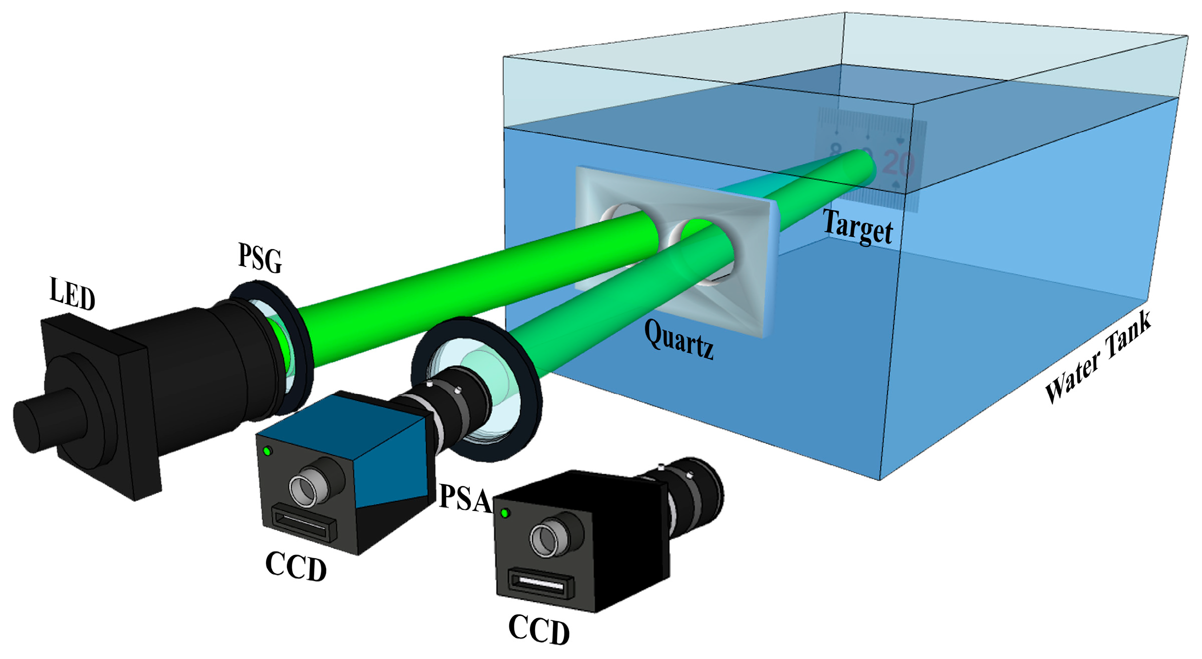
As shown in Figure 2, water and skimmed milk were added into a tank measuring 180 cm × 60 cm × 60 cm. The water level was allowed to rise to 30 cm, at which point 160 mL and 200 mL of milk were added, which created two scattering media with different turbidities. According to [28], the mixture of milk and water can be used to simulate an actual seawater environment. The concentrations of milk in the two media were 0.64 g/L and 0.8 g/L, respectively. In this way, the scattering coefficients were 0.059/cm and 0.074/cm, respectively. All the targets were 80 cm from the front wall of the water tank, corresponding to 4.74 and 5.92 scattering mean lengths in the two turbid media, separately.

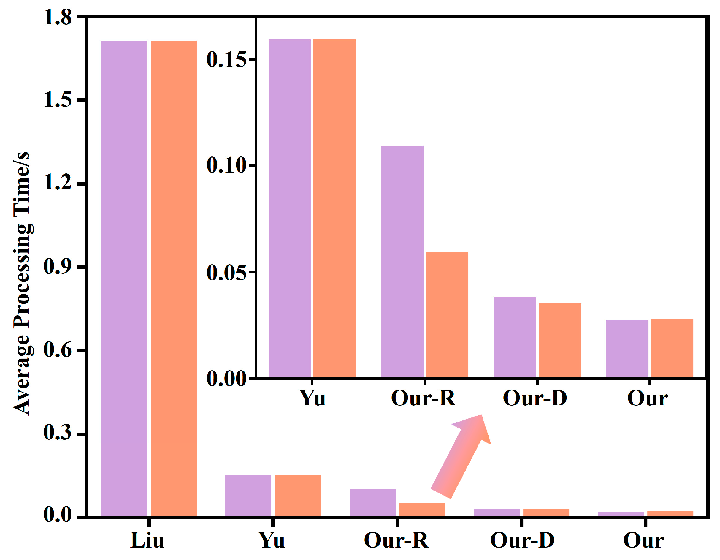
The imaging devices were placed in front of the water tank. LED and PSG (Polarization State Generator, DAHENG IMAGING, Beijing, China) made up the light source, and a beam of light with a central wavelength of 550 nm was emitted to provide active polarized illumination. The image acquisition unit adapted to the motion state of the target. Specifically, a PSA (Polarization State Analyzer, DAHENG IMAGING, Beijing, China) and an intensity camera (DAHENG IMAGING MER2-502-79U3M, DAHENG IMAGING, Beijing, China) were utilized to obtain images of static targets. During dynamic imaging, the video was recorded by the polarimetric camera (FLIR BFS-U3-51S5P-C, Teledyne FLIR, Shanghai, China) with an exposure time of 0.005 s.

3.2. Imaging Results of Different Methods in Static Imaging

The flowchart in Figure 1 can serve as simple proof of the effectiveness of the proposed method in coping with targets with complex polarization characteristics. Next, this composite target is taken apart to further validate the applicability of our approach to targets with single polarization characteristics. Imaging results of the steel ruler with weak depolarization abilities are shown in Figure 3.

As can be seen, the haze formed by the backscattered light dramatically attenuates the clarity of intensity images. To make matters worse, the target is almost invisible in the strong scattering environment, which is the last thing to be expected. CLAHE (Contrast Limited Adaptive Histogram Equalization) stretches the histogram of the image and alleviates the negative consequences of scattering. Though the haze still exists in the image, patterns such as numbers can be vaguely seen. The rapid PDI method created by Tian exploits the differential operation between S₁ and S₂; however, the spatial variation of backscattered light is not considered. Therefore, it is not surprising that imaging is limited with such a large field of view. Zhao’s method is based on a polarization descattering model, and the optimal values of the polarization parameters are obtained by a genetic algorithm, which provides excellent performance in low-scattering environments. However, as turbidity increases, the descattering performance decreases. In contrast, our method yields the most satisfactory results. Through the differential computation between the total intensity and the global distribution of backscattered light, the haze is effectively eliminated, meaning that tiny details can be easily distinguished. Notably, in the enlarged views, the chosen motifs are displayed with exceptional clarity. Meanwhile, stronger scattering does not prevent our method from achieving excellent descattering performance. The thin scale lines can still be retrieved from the dense haze. All these prove the effectiveness and stability of the proposed method.

Figure 4 shows the imaging results and enlarged views of another ruler that is made of plastic. Light is mainly diffusely reflected on the surface of this sticky ruler, which accounts for the loss of polarization-preserving abilities. No apparent changes can be found in the results of intensity imaging and CLAHE. As before, the latter mitigates the veiling effects present in the former. However, Tian’s method suffers a major setback. According to the aforementioned derivation, the differential operation between the polarized components is not suitable for targets with strong depolarization abilities. Unfortunately, Tian’s method falls into this unfavorable situation and meets its Waterloo. Significant inhomogeneities appear in Zhao’s results due to the fact that the spatial variation of the polarization properties is not taken into account. However, the descattering effect of this method is good and is maintained in high-turbidity environments. Thanks to the differential computation between S₀ and the estimation result of the backscatter, our method performs well despite the failure of previous PDI methods, consistently achieving effective elimination of backscattered light regardless of scattering intensity. The prominent imaging effects and stability of the proposed method are verified again. Meanwhile, it can be argued that the proposed method applies to targets with various polarization characteristics. The scope of its application is not only extended to targets with strong depolarization abilities, but it goes a step further and makes the method applicable to composite targets with complex polarization characteristics. Therefore, all of these facts present powerful proof of our method’s greater applicability.

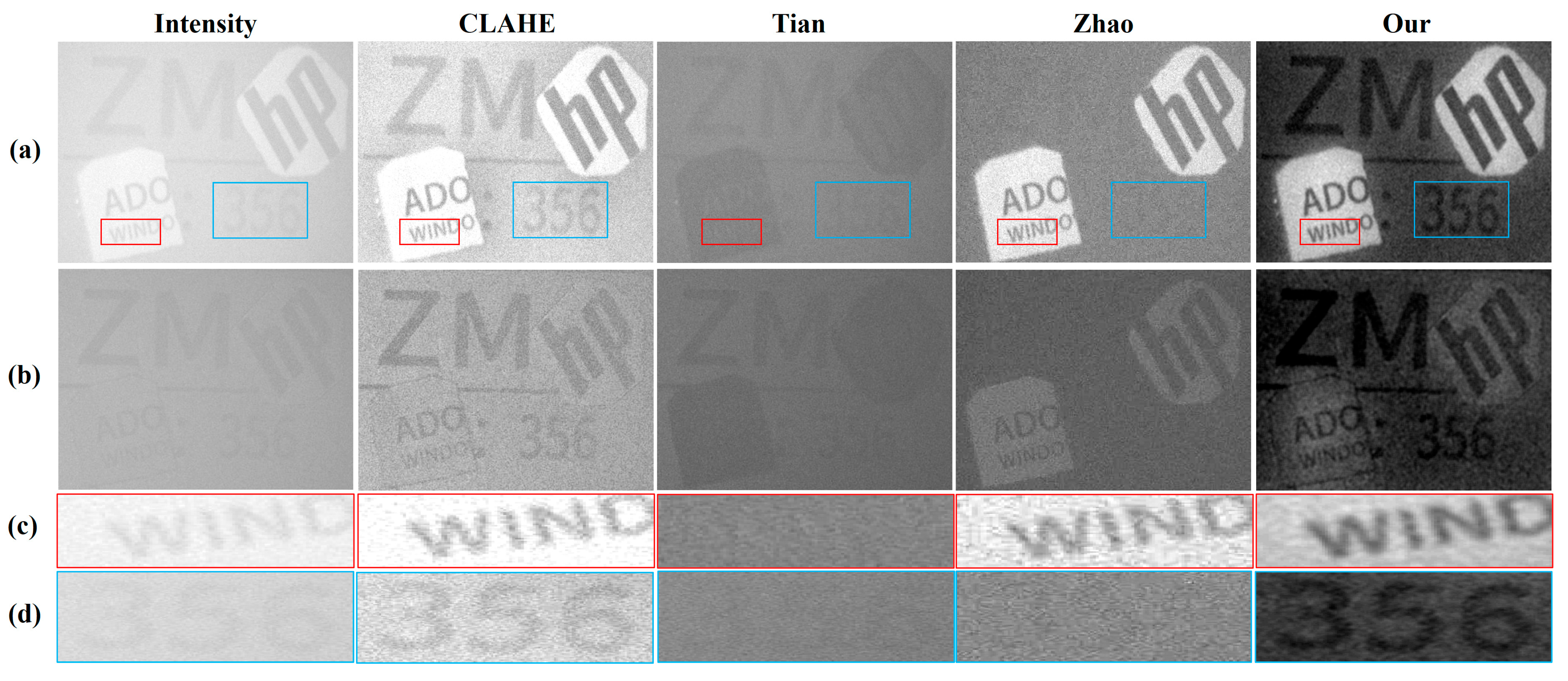
In Figure 5, an imaging target with complex polarization characteristics further validates the proposed method. This composite target includes three targets with different polarization characteristics and materials. The lowermost target is a piece of iron, and light mainly reflects specularly off the surface, making it a highly polarized target. The two targets above it are disc fragments where light is mainly diffusely reflected on the surface, making them lowly polarized targets.

To reduce the bias of subjective evaluation, two parameters, contrast (C) and Enhancement Measure Evaluation (EME), were used as the basis for quantitative comparison. According to [31], the definition of C is as follows:

$$C={\displaystyle \frac{\sigma }{\overline{I}}}={\displaystyle \frac{\sqrt{\frac{1}{M\times N}{\displaystyle \sum _{i=1}^M{\displaystyle \sum _{j=1}^N{\left[I(i,j)-\overline{I}\right]}^2}}}}{\frac{1}{M\times N}{\displaystyle \sum _{i=1}^M{\displaystyle \sum _{j=1}^{N}I(i,j)}}}}.$$

(16)

where σ is the standard deviation of the grayscale values of the pixels in the image; $\overline{I}$ is the average gray value of the image; M and N represent the numbers of rows and columns, respectively; and I(i,j) denotes the gray value of the pixel located in the ith row and jth column. The formula of EME is given in [32]:

$$\mathrm{EME}=\left|{\displaystyle \frac{1}{k_1{k}_2}}{\displaystyle \sum _{l_1=1}^{k_1}{\displaystyle \sum _{l_2=1}^{k_2}20\log \frac{I_{\max ;l_1,l_2}}{I_{\min ;l_1,l_2}+q}}}\right|.$$

(17)

Here, k₁ and k₂ indicate that the image is divided into k₁ × k₂ blocks; l₁ and l₂ are the serial numbers of the corresponding horizontal and vertical image blocks, respectively; and $I_{\max ;l_1,l_2}$ and $I_{\min ;l_1,l_2}$ denote the maximum and minimum gray values of all the pixels in the image block. q is set to 0.0001 to avoid denominators of 0.

As shown in Figure 5, the imaging effects of intensity imaging and CLAHE still do not change much. The visual effect of the latter is enhanced, but backscattered light is not eliminated. This is shown in

Table 1. Evaluation parameters of imaging results. (Bolded red indicates maximum value).

Parameter	Turbidity	Method
		Intensity	CLAHE	Tian	Zhao	Our
C	Low	0.0589	0.1291	0.0788	0.2419	0.5892
	High	0.0401	0.0809	0.0655	0.1028	0.4292
EME	Low	1.5263	4.7902	2.8995	6.8611	12.7797
	High	1.2550	3.9540	2.6624	4.8859	11.0614

by a slight increase in the parameter values. The imaging results of Tian’s method and Zhao’s method are somewhat complementary. As mentioned earlier, Tian’s method is not suitable for lowly polarized targets, which makes the area where the discs are located black. Zhao’s method does not take into account the distribution of polarization characteristics, so it can only work on targets with the same polarization characteristics. Consequently, the imaging effect of the iron sheet is very poor. In contrast, our method continues to show excellent imaging effects. Regardless of the polarization characteristics of the target, the backscattered light can be eliminated to a great extent. Various patterns have a clear display, both in the imaging results and in the enlarged views. In particular, effective elimination can be maintained in high-turbidity environments. Consistent with these manifestations, the values of C and EME are significantly improved, providing reliable and objective data for the improvement of imaging quality.

Based on the above, it can be argued that our method can obtain prominent descattering effects, greater applicability, and good stability simultaneously.

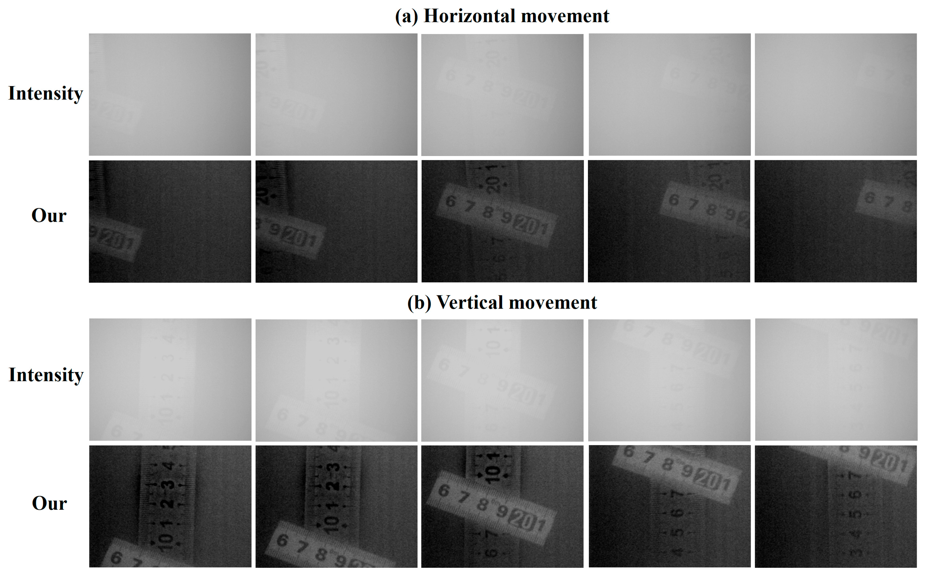
3.3. The Dynamic Imaging Results

To assess the dynamic imaging effects of the proposed method, the composite target with complex polarization characteristics was selected for video shooting. It should be mentioned that in practice, contingencies happen occasionally. Therefore, some accidental factors including uneven illumination, strong specular reflection, and target jitter were also captured in the videos, which assists in proving the stability of the proposed approach in unexpected situations. The dynamic imaging results are shown in Figure 6.

The results of the quantitative assessment, presented as curves, are shown in Figure 7.

As can be seen, in the face of challenges stemming from both the complex polarization characteristics of the target and dynamic imaging, which has been a major issue for previous PDI approaches, the performance of the proposed method is surprising enough. The haze produced by the backscattered light is significantly decreased, making the target that is barely visible in intensity images readily apparent. In particular, tiny details such as the scale lines can be clearly distinguished. Consistent with these manifestations, the values of C and EME have increased considerably. Each curve of our imaging results is at the top, pulling away from the intensity curves below by a large distance. The maximum difference is 0.4203 and 9.2220, which implies that our method improves C and EME by a factor of 7.3 and 12.6, respectively. Even with the worst effect as the metric, the improvement is about 2.4 times, which is also commendable. Given this, the excellent dynamic imaging capabilities of the proposed method are well proven.

Next, a transversal comparison between each frame was performed to analyze the stability of our approach. As mentioned earlier, some intentional contingencies were included in the videos. The target jitter and uneven illumination can be found without trouble. The first factor causes the target to deviate from the regular trajectory motion, which is acceptable given that there will always be targets that do not move along a predictable path. However, this might produce the unfavorable consequence of being out of focus. As can be seen, except for the first frame, the rest of the frames are in a state of no precise focus, which certainly adds to the existing blurriness of the intensity image. The detrimental effects of uneven illumination manifest as discrepancies in brightness. This phenomenon is rather similar to the consequences of strong specular reflection. But there is a difference between the two factors, as the latter only produces strong brightness. By comparison, these three contingencies have minimal impact on the proposed approach. In our results, the targets blurred by backscatter and target jitter regain clarity, and the visual effects of the image are greatly improved. Uneven illumination is no longer apparent because the spatial variation of backscattered light is estimated. It may be noted that there are black numbers with white imprints in the upper middle of the first two images in Figure 5b, which look out of place with the surrounding distribution. However, this is determined by the properties of the low-pass filtering. Strong specular reflections are set in the area occupied by the numbers ‘3’ and ‘2’, leading to a dramatic increase in brightness. At this point, a sudden change in intensity is produced and transformed into the high-frequency component. Consequently, this region is eliminated along with the backscattered light. Fortunately, the target information is kept intact and even accentuated by the black patterns and white imprints. The reason for this abnormal manifestation is understandable, as the area is brighter and so is the intensity after treatment. As a result, the white imprints are formed. Since this has little effect on the imaging results, it can be left alone. Meanwhile, in the context of the dilemmas faced by the previous methods, the response of our approach to the dual challenge is even more valuable. Therefore, it can be argued that our method could be free from unexpected conditions and has good stability.

Based on the above analysis, the prominent imaging effects, greater applicability, and good stability are well documented, which is a big step toward practical application.

4. Discussion

4.1. The Determination of the Optimal Proportional Factor

The role played by the proportional factor α is amplifying the intensity of B_p to approximate the total intensity of backscatter. Hence, the value of α is critical for imaging quality. To explore the direct impact of this factor, a series of imaging results for further analysis were generated by substituting different values of α, which are shown in Figure 8.

From Figure 8, the curve of C can be divided into two parts. As the reciprocal of P_scat, the value of α is larger than 1. As α increases, the descattering effect becomes more pronounced. More and more haze is eliminated and imaging clarity rises rapidly. Correspondingly, the value of C increases likewise. The reason for these obvious elevations is that the magnified B_p is generated. Accompanied by amplification effects, the estimated result gradually approaches the total intensity of the backscattered light. Hence, there is no doubt that the differential operation becomes the nemesis of the haze. Unfortunately, the value of α cannot be converged. With a continuous increase in amplification, the estimation result may outweigh the ground truth. As a result, the image is occupied by pixels with gray values of 0. In contrast, the steel ruler cannot withstand the pressure, making the area in which it is located turn black. Initially, the values of these pixels are indeed 0. Nevertheless, subsequent zero-valued pixels result from truncating negative values. Under these circumstances, the result cannot be displayed properly, only by way of assigning pseudo-colors. This situation, however, does not affect the calculation of C. Moreover, it seems to cause the curve to soar, except that this is not meaningful at all.

Hence, a reasonable range of α can be deduced as follows:

$$1<\alpha <{\alpha }_{up}.$$

(18)

Here, ${\alpha }_{up}$ represents the upper bound of the value. When the value of α is equal to the ratio of S₀ and B_p, T is calculated to be 0. On the one hand, this means that the backscattered light is completely eliminated and T is restored to its true value, which is the desired goal. On the other hand, this process may also cause values that are not 0 to become 0, causing the target information to be eliminated. Hence, to maintain the integrity of the target information, the value of α cannot be more than the ratio of S₀ and B_p. Meanwhile, considering the spatial variation of pixel values, the ratio of the mean values of S₀ and B_p turns into the most suitable candidate for the upper limit. It can be inferred that for those positions that should be 0, the value of α must be less than the upper limit. Therefore, the formula of ${\alpha }_{up}$ is as follows.

$${\alpha }_{up}={\displaystyle \frac{\frac{1}{M\times N}{\displaystyle \sum _{i=1}^M{\displaystyle \sum _{j=1}^N{S}_0(i,j)}}}{\frac{1}{M\times N}{\displaystyle \sum _{i=1}^M{\displaystyle \sum _{j=1}^N\sqrt{S_{1B}^2(i,j)+S_2^2(i,j)}}}}}={\displaystyle \frac{\overline{S_0}}{\overline{B_p}}}.$$

(19)

As far as we are concerned, in this suitable range, all values have an amplifying effect. Hence, there is a degree of freedom in the value of this parameter. To ensure descattering effects, the value of α should be as large as possible. Meanwhile, to ensure the integrity of the target information, the value should not be taken too close to the upper limit. Under these circumstances, the interval is divided into four parts, and the third node can be selected as the optimum directly, i.e., the following:

$${\alpha }_{opt}={\displaystyle \frac{\frac{1+{\alpha }_{up}}{2}+{\alpha }_{up}}{2}}={\displaystyle \frac{1+3{\alpha }_{up}}{4}}.$$

(20)

This best value not only prevents a large number of zero-valued pixels from appearing so that the erroneous elimination of target information is avoided, but also makes pixels that would otherwise be zero recover their original value, thus ensuring descattering effects. Meanwhile, the acquisition of this best value is considered in terms of ensuring the descattering effect as well as preserving the target information, and the whole process conforms to the laws of physics. More importantly, the tedious iterative process of finding the optimum can be avoided, which makes it possible for dynamic imaging.

4.2. The Advantages of Imaging Time

In the field of dynamic imaging, the imaging time is of great importance. If the imaging time is not up to par, then dynamic imaging cannot be performed. An analytical comparison of the different methods’ processing times is shown in Figure 9.

Each frame with a size of 1024 × 1224 in the videos was processed via the proposed approach. The CPU of the computer is AMD R5-3600. As for the remaining four methods used for comparison, the processing is identical or similar. In other words, there are few discrepancies between all methods in terms of data volume, hardware, etc. In this case, the proposed method takes the least amount of time. For the videos of horizontal and vertical movements, disregarding the image reading as well as other pre-processing steps, the processing is timed and then the average of five results is taken. Consequently, the average processing times are 0.0280 s and 0.0286 s, respectively. Compared to other methods, the curtailment has a maximum of 98.37%. For this reason, the color bars are hard to see without looking at the enlarged view. When the highest bars are phased out, our dynamic method chases the proposed method closely. However, with the addition of an exposure time that is 0.005 s, the generalized upper bound (0.04 s) makes the competitive situation immediately apparent. Therefore, with these obvious advantages in imaging time, the proposed method is fully capable of fulfilling actual dynamic imaging requirements.

In addition to the above, much attention should be paid to the next issue. The image size as well as the operating environment of our method are universal, making all methods essentially the same in terms of spatial complexity, etc. Meanwhile, the low-pass filtering is utilized by Yu’s method, our-R method, and the proposed method. However, the average processing time is quite different. Iterative operations are the biggest culprit behind this. Fortunately, with direct substitution of the optimal proportional factor, this time-wasting step is avoided by our approach. On this basis, operations such as parallel processing also provide some help in reducing the imaging time. Therefore, the proposed method emerges as the winner in the race of imaging time. As for the nuance produced by different movements, it may be due to the variation of the area occupied by the target in the image.

5. Conclusions

To sum up, with the Stokes vector, the differential operation between the total intensity of light and the estimation result of backscatter achieves the goal of clear imaging. At the same time, underwater dynamic polarization-difference imaging with greater applicability becomes available. Through a series of experimental results and analytical comparisons, the prominent imaging effects, real-time characteristics, greater applicability, and good stability of the proposed method are fully proven, indicating a reassuring underwater dynamic imaging performance. Thanks to these advantages, the difficult process can be carried out even when imaging moving targets with various polarization characteristics in strong scattering environments. Therefore, it can be expected that our method will be beneficial in practical applications.

Currently, the processing of captured videos ultimately boils down to incomplete dynamic imaging. In the future, the associated hardware will be further developed to enable true underwater imaging.

References

1. Fayaz, S.; Parah, S.A.; Qureshi, G.J.; Lloret, J.; Ser, J.D.; Muhammad, K. Intelligent Underwater Object Detection and Image Restoration for Autonomous Underwater Vehicles. IEEE Trans. Veh. Technol. 2024, 73, 1726–1735. [Google Scholar] [CrossRef]
2. Amer, K.O.; Elbouz, M.; Alfalou, A.; Brosseau, C.; Hajjami, J. Enhancing underwater optical imaging by using a low-pass polarization filter. Opt. Express 2019, 27, 621–643. [Google Scholar] [CrossRef] [PubMed]
3. Wu, H.; Zhao, M.; Xu, W. Underwater De-scattering Imaging by Laser Field Synchronous Scanning. Opt. Lasers Eng. 2020, 126, 8. [Google Scholar] [CrossRef]
4. Wang, M.; Wang, X.; Zhang, Y.; Sun, L.; Lei, P.; Yang, Y.; Chen, J.; He, J.; Zhou, Y. Range-intensity-profile prior dehazing method for underwater range-gated imaging. Opt. Express 2021, 29, 7630–7640. [Google Scholar] [CrossRef]
5. Jeon, D.S.; Meuleman, A.; Baek, S.H.; Kim, M.H. Polarimetric iToF: Measuring High-Fidelity Depth Through Scattering Media. In Proceedings of the 2023 IEEE/CVF Conference on Computer Vision and Pattern Recognition (CVPR), Vancouver, BC, Canada, 17–24 June 2023; pp. 12353–12362. [Google Scholar]
6. Guo, E.; Jiang, J.; Shi, Y.; Bai, L.; Han, J. Unsupervised underwater imaging based on polarization and binocular depth estimation. Opt. Express 2024, 32, 9904–9919. [Google Scholar] [CrossRef]
7. Wu, L.; Zhang, X.; Chang, J.; Li, B. Underwater polarization image de-scattering utilizing a physics-driven deep learning method. Opt. Express 2024, 32, 30670–30686. [Google Scholar] [CrossRef]
8. Qian, J.; Li, J.; Wang, Y.; Liu, J.; Wang, J.; Zheng, D. Underwater image recovery method based on hyperspectral polarization imaging. Opt. Commun. 2021, 484, 126691. [Google Scholar] [CrossRef]
9. Treibitz, T.; Schechner, Y.Y. Active Polarization Descattering. IEEE Trans. Pattern Anal. Mach. Intell. 2009, 31, 385–399. [Google Scholar] [CrossRef]
10. Garcia, M.; Davis, T.; Blair, S.; Cui, N.; Gruev, V. Bioinspired polarization imager with high dynamic range. Optica 2018, 5, 1240–1246. [Google Scholar] [CrossRef]
11. Liu, T.; Guan, Z.; Li, X.; Cheng, Z.; Han, Y.; Yang, J.; Li, K.; Zhao, J.; Hu, H. Polarimetric underwater image recovery for color image with crosstalk compensation. Opt. Lasers Eng. 2020, 124, 6. [Google Scholar] [CrossRef]
12. Zhang, H.; Gong, J.; Ren, M.; Zhou, N.; Wang, H.; Meng, Q.; Zhang, Y. Active Polarization Imaging for Cross-Linear Image Histogram Equalization and Noise Suppression in Highly Turbid Water. Photonics 2023, 10, 19. [Google Scholar] [CrossRef]
13. Wang, C.; Wu, Z.; Han, Z.; Wang, J.; Hu, H.; Li, X. Rethinking of Underwater Image Restoration Based on Circularly Polarized Light. Photonics 2024, 11, 14. [Google Scholar] [CrossRef]
14. Cameron, D.A.; Pugh, E.N. Double cones as a basis for a new type of polarization vision in vertebrates. Nature 1991, 353, 161–164. [Google Scholar] [CrossRef] [PubMed]
15. Rowe, M.P.; Pugh, E.N.; Tyo, J.S.; Engheta, N. Polarization-difference imaging—A biologically inspired technique for observation through scattering media. Opt. Lett. 1995, 20, 608–610. [Google Scholar] [CrossRef] [PubMed]
16. Tyo, J.S. Enhancement of the point-spread function for imaging in scattering media by use of polarization-difference imaging. J. Opt. Soc. Am. A-Opt. Image Sci. Vis. 2000, 17, 1–10. [Google Scholar] [CrossRef] [PubMed]
17. Walker, J.G.; Chang, P.C.Y.; Hopcraft, K.I. Visibility depth improvement in active polarization imaging in scattering media. Appl. Opt. 2000, 39, 4933–4941. [Google Scholar] [CrossRef]
18. Guan, J.; Zhu, J. Target detection in turbid medium using polarization-based range-gated technology. Opt. Express 2013, 21, 14152–14158. [Google Scholar] [CrossRef]
19. Zhu, Y.; Shi, J.; Yang, Y.; Zeng, G. Polarization difference ghost imaging. Appl. Opt. 2015, 54, 1279–1284. [Google Scholar] [CrossRef]
20. Guan, J.; Zhu, J.; Tian, H.; Hou, X. Real-time polarization difference underwater imaging based on Stokes vector. Acta Phys. Sin. 2015, 64, 141–147. [Google Scholar]
21. Tian, H.; Zhu, J.; Tan, S.; Zhang, Y.; Zhang, Y.; Li, Y.; Hou, X. Rapid underwater target enhancement method based on polarimetric imaging. Opt. Laser Technol. 2018, 108, 515–520. [Google Scholar] [CrossRef]
22. Wang, H.; Hu, H.; Jiang, J.; Li, J.; Li, X.; Zhang, W.; Cheng, Z.; Liu, T. Polarization differential imaging in turbid water via Mueller matrix and illumination modulation. Opt. Commun. 2021, 499, 8. [Google Scholar] [CrossRef]
23. Wang, J.; Wan, M.; Gu, G.; Qian, W.; Ren, K.; Huang, Q.; Chen, Q. Periodic integration-based polarization differential imaging for underwater image restoration. Opt. Lasers Eng. 2022, 149, 8. [Google Scholar] [CrossRef]
24. Wei, Y.; Han, P.; Liu, F.; Shao, X. Estimation and removal of backscattered light with nonuniform polarization information in underwater environments. Opt. Express 2022, 30, 40208–40220. [Google Scholar] [CrossRef] [PubMed]
25. Huang, B.; Liu, T.; Hu, H.; Han, J.; Yu, M. Underwater image recovery considering polarization effects of objects. Opt. Express 2016, 24, 9826–9838. [Google Scholar] [CrossRef] [PubMed]
26. Wang, J.; Wan, M.; Cao, X.; Zhang, X.; Gu, G.; Chen, Q. Active non-uniform illumination-based underwater polarization imaging method for objects with complex polarization properties. Opt. Express 2022, 30, 46926–46943. [Google Scholar] [CrossRef]
27. Deng, J.; Zhu, J.; Li, H.; Zhang, X.; Guo, F.; Hou, X. Real-time underwater polarization imaging without relying on background. Opt. Lasers Eng. 2023, 169, 10. [Google Scholar] [CrossRef]
28. Piederriere, Y.; Boulvert, F.; Cariou, J.; Le Jeune, B.; Guern, Y.; Le Brun, G. Backscattered speckle size as a function of polarization: Influence of particle-size and -concentration. Opt. Express 2005, 13, 5030–5039. [Google Scholar] [CrossRef]
29. Reza, A.M. Realization of the Contrast Limited Adaptive Histogram Equalization (CLAHE) for real-time image enhancement. VLSI Signal Process. 2004, 38, 35–44. [Google Scholar] [CrossRef]
30. Zhao, Y.; He, W.; Ren, H.; Li, Y.; Fu, Y. Polarization descattering imaging through turbid water without prior knowledge. Opt. Lasers Eng. 2022, 148, 6. [Google Scholar] [CrossRef]
31. Schechner, Y.Y.; Karpel, N. Recovery of underwater visibility and structure by polarization analysis. IEEE J. Ocean. Eng. 2005, 30, 570–587. [Google Scholar] [CrossRef]
32. Agaian, S.S.; Panetta, K.; Grigoryan, A.M. Transform-based image enhancement algorithms with performance measure. IEEE Trans. Image Process. 2001, 10, 367–382. [Google Scholar] [CrossRef] [PubMed]
33. Liu, L.; Li, X.; Yang, J.; Tian, X.; Liu, L. Fast image visibility enhancement based on active polarization and color constancy for operation in turbid water. Opt. Express 2023, 31, 10159–10175. [Google Scholar] [CrossRef] [PubMed]
34. Yu, T.; Wang, X.; Xi, S.; Mu, Q.; Zhu, Z. Underwater polarization imaging for visibility enhancement of moving targets in turbid environments. Opt. Express 2023, 31, 459–468. [Google Scholar] [CrossRef] [PubMed]
35. Deng, J.; Zhu, J.; Li, H.; Liu, X.; Guo, F.; Zhang, X.; Hou, X. Underwater dynamic polarization imaging without dependence on the background region. Opt. Express 2024, 32, 5397–5409. [Google Scholar] [CrossRef]
Figure 1. A flowchart of the proposed method.
Photonics 11 01069 g001
Figure 2. The experimental setup for underwater polarization imaging. The intensity camera is on the left and the polarimetric camera is on the right.
Photonics 11 01069 g002
Figure 3. Imaging results of the highly polarized steel ruler in scattering media with (a) low and (b) high levels of turbidity, which were generated by intensity imaging through CLAHE [29], Tian’s method [21], Zhao’s method [30], and our method. The enlarged views of the regions marked by (c) red and (d) blue rectangles are placed at the bottom.
Photonics 11 01069 g003
Figure 4. Imaging results and enlarged views of the lowly polarized sticky ruler in two scattering media with different turbidities. The meanings of (ad) are the same as before. The enlarged views of the regions marked by red and blue rectangles are placed at the bottom.
Photonics 11 01069 g004
Figure 5. Imaging results and enlarged views of another composite target in two scattering media with different turbidities. The meanings of (ad) are the same as before. The enlarged views of the regions marked by red and blue rectangles are placed at the bottom.
Photonics 11 01069 g005
Figure 6. Key frames of the original and processed videos that indicate the (a) horizontal and (b) vertical movement of the composite target. For the former, the 6th, 11th, 35th, 55th, and 65th frames were chosen. For the latter, the ordinal numbers are 1, 11, 35, 60, and 70. The full video can be found in Video S1.
Photonics 11 01069 g006
Figure 7. The quantitative evaluation results of the images in Figure 6. (a) Horizontal and (b) vertical movement. The left and right axes represent the values of C and EME, separately.
Photonics 11 01069 g007
Figure 8. Imaging results generated by substituting different values of α. Dashed lines indicate abnormal imaging. Images that cannot be displayed are indicated by pseudo-colors. The middle segment indicating normal imaging is shown enlarged and placed in the upper left corner with the axes on the left. The image with blue borders is the result of intensity imaging. Because more attention is paid to the overall imaging effects, only C is used as a means of judgment.
Photonics 11 01069 g008
Figure 9. The average processing times of different methods. The first two sets of color columns are from the data of Liu [33] and Yu [34], respectively. The last three sets belong to us, and are from the real-time method [27], the dynamic method [35], and the proposed method. For better exhibition, the last four sets of lower color bars are shown enlarged and placed in the upper right corner. Since there are methods with two processing times, two colors are used to represent them. For consistency in displaying the effect, these two colors are still used to represent the single times of other methods.
Photonics 11 01069 g009