Online Optical Axis Parallelism Measurement Method for Continuous Zoom Camera Based on High-Precision Spot Center Positioning Algorithm

Abstract

Ensuring precise alignment of the optical axis is critical for achieving high-quality imaging in continuous zoom cameras. However, existing methods for measuring optical axis parallelism often lack accuracy and fail to assess parallelism across the entire focal range. This study introduces an online measurement method designed to address these limitations by incorporating two enhancements. First, image processing methodologies enable sub-pixel-level extraction of the spot center, achieved through improved morphological processing and the incorporation of an edge tracing algorithm. Second, measurement software developed using Qt Creator can output real-time data on optical axis parallelism across the full focal range post-measurement. This software features a multi-threaded architecture that facilitates the concurrent execution of image acquisition, data processing, and serial communication. Experimental results derived from simulations and real data indicate that the maximum average error in extracting the center of the spot is 0.13 pixels. The proposed system provides critical data for optical axis calibration during camera adjustment and inspection.

1. Introduction

Continuous zoom cameras possess a focal length that can vary continuously within a specific range, enabling imaging measurements of objects at different distances [1]. However, due to manufacturing and assembly constraints, lens groups may shift during zooming, resulting in optical axis misalignment and subsequent degradation of image quality [2]. Measuring the parallelism of the lens’s optical axis during the debugging and testing stages is essential for effective optical axis calibration.

Traditional methods for measuring optical axis parallelism include the collimator method, projection target method, laser optical axis meter method, and pentaprism method [3,4,5,6]. As optoelectronic systems become increasingly complex and demands for measurement accuracy and efficiency rise, these traditional methods have proven inadequate. Among these techniques, the collimator method offers high measurement precision and is commonly employed in laboratory testing instruments [7]. Consequently, several researchers have proposed innovative testing methods and systems based on the collimator method [8,9,10,11]. These studies focus on various optical systems, utilizing image processing technology to extract the target center and employing computer software to assess optical axis parallelism.

In the case of continuous zoom cameras, traditional methodologies involve capturing images at multiple focal lengths. The offset of the target center relative to the image center is visually assessed by the human eye. This method is prone to significant subjective error and does not reflect optical axis parallelism across the entire focal range. In 2023, Kong et al. [12] proposed a method for measuring optical axis parallelism based on a skeleton thinning algorithm. This approach addresses issues such as varying image intensity and changing crosshair width during zooming. It continuously calculates the offset of the target center relative to the image center. However, this method has a detection error of 1 pixel when extracting the target center and measures the offset only offline. This limitation prevents the real-time acquisition of optical axis parallelism data.

This paper proposes a measurement method for optical axis parallelism in continuous zoom cameras. The measurement software incorporates a circular target center extraction algorithm and employs multithreaded development to continuously and automatically measure optical axis parallelism during zooming. The main contributions of this paper are outlined as follows.

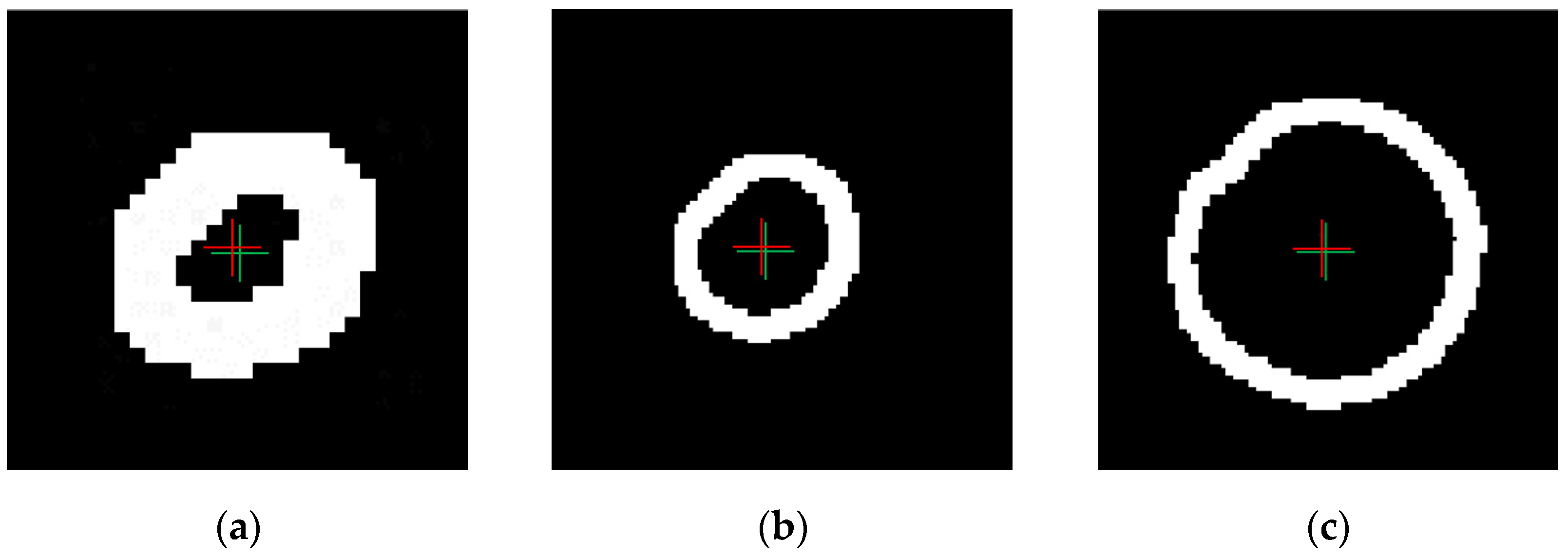
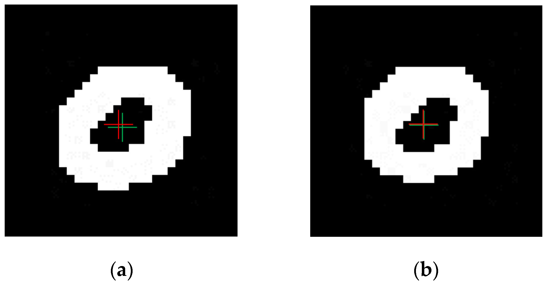
• This paper presents a morphology-based method for extracting the spot center. A novel structuring element is designed to dilate the spot, followed by implementing an edge tracing algorithm to extract the contour of the binary spot. This method achieves sub-pixel accuracy in spot center extraction and exhibits excellent repeatability.
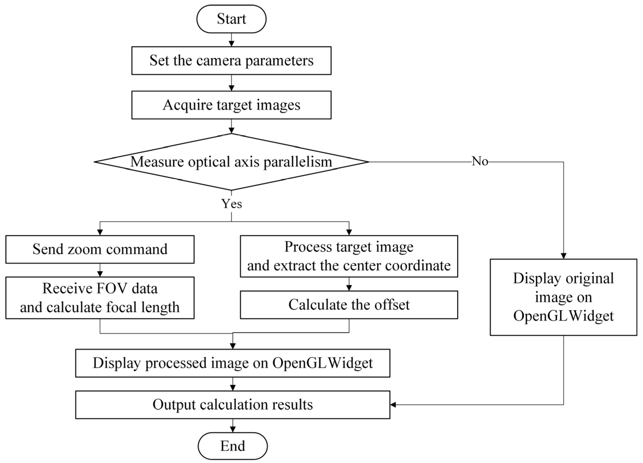
• The measurement software is capable of calculating and outputting the optical axis parallelism across the entire focal range. This software continuously acquires target images during zooming, extracts the coordinate of the target center, and automatically retrieves focal length data via serial communication.
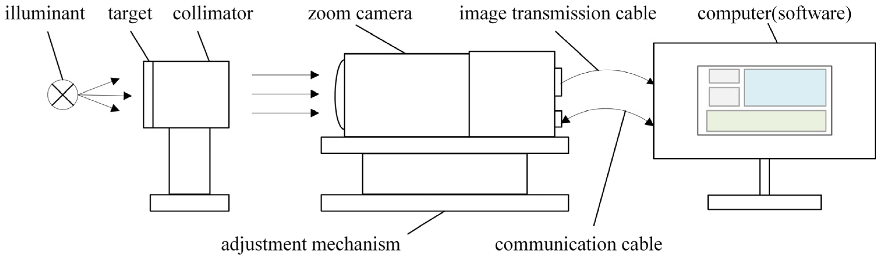
• An experimental platform was established to conduct tests that validate the accuracy of the proposed algorithm and assess the feasibility of the optical axis parallelism measurement system.

This paper is organized as follows: Section 2 introduces the target center extraction algorithm. Section 3 describes the design of the optical axis parallelism measurement software. Section 4 presents and discusses the experimental results. Finally, Section 5 concludes the paper and future directions.

2. Algorithm Research

2.1. Traditional Center Positioning Algorithm

2.1.1. Hough Transform Method

The Hough transform utilizes point-line duality to map information from image space to parameter space, converting the extraction of curves into a peak detection problem [13]. We assume that the parametric equation of the curve to be detected is

$$f\left(a_1,a_2,\cdots ,a_n,x,y\right)=0$$

(1)

where $a_1,a_2,\cdots ,a_n$ denote the shape parameter and $\left(x,y\right)$ represents the image point coordinate. The Hough transform substitutes each contour point from the image space into Equation (1). The computed results undergo voting at quantized points in the parameter space $\left(a_1,a_2,\cdots ,a_n\right)$ based on proximity. When the vote count surpasses a specified threshold, the curve parameters can be determined. For circular curves, the analytical expression is

$${\left(x-x_0\right)}^2+{\left(y-y_0\right)}^2=R^2$$

(2)

with the parameter space defined as $\left(x_0,y_0,r\right)$, where $\left(x_0,y_0\right)$ represents the circle center and R is the radius.

When applying the Hough transform to detect circles, it is necessary to discretize the parameter space. Each contour point then casts a vote in the three-dimensional parameter space, a process that is computationally intensive and time-consuming [14]. Furthermore, the Hough transform requires high-quality edge shapes of the light spot. The accuracy of circular contour detection decreases when the spot exhibits defects.

2.1.2. Grayscale Centroid Method

The grayscale centroid method employs a weighted approach, utilizing grayscale values as weights [15]. Supposing the image size is $m\times n$, the grayscale value of each pixel is denoted as $I\left(x,y\right)$. The spot center can be expressed as

$$\left\{\begin{array}{c}{x}_0={\displaystyle \frac{{\displaystyle \sum _{i=1}^m{\displaystyle \sum _{j=1}^{n}i\cdot I\left(x,y\right)}}}{{\displaystyle \sum _{i=1}^m{\displaystyle \sum _{j=1}^{n}I\left(x,y\right)}}}}\\ y_0={\displaystyle \frac{{\displaystyle \sum _{i=1}^m{\displaystyle \sum _{j=1}^{n}j\cdot I\left(x,y\right)}}}{{\displaystyle \sum _{i=1}^m{\displaystyle \sum _{j=1}^{n}I\left(x,y\right)}}}}\end{array}\right.$$

(3)

This method determines the spot center using pixels with higher gray values. Its accuracy is influenced by the degree of energy concentration in the light spot. When the brightness is scattered, the extraction precision deteriorates [16]. Consequently, although the grayscale centroid method is computationally straightforward, it is susceptible to noise and has poor anti-interference capability.

2.1.3. Least Squares Circle Fitting Method

The least squares method is a mathematical optimization technique that identifies the best-fitting function for a given dataset by minimizing the sum of the squares of the errors [17]. The least squares circle fitting method is a statistical detection approach represented by the circular fitting curve below:

$${\left(x-x_0\right)}^2+{\left(y-y_0\right)}^2=R^2$$

(4)

where $\left(x_0,y_0\right)$ represents the coordinates of the center and R is the radius. The least squares method is employed to determine the optimal estimates of the parameters of the objective function. Aiming to minimize the sum of the squared distances $f_i$ from the measurement points $\left(x_i,y_i\right)$ to the circle:

$$f_i={{\displaystyle \sum _{i=1}^N\left(\sqrt{{\left(x_i-x_0\right)}^2+{\left(y_i-y_0\right)}^2}-R\right)}}^2$$

(5)

To simplify the description, let $d=\sqrt{{\left(x_i-x_0\right)}^2+{\left(y_i-y_0\right)}^2}$, and convert the problem of solving for ${\left(d-R\right)}^2$ into finding the minimum of $\left(d^2-R^2\right)$, thus transforming the nonlinear least squares problem into a linear one. Define $a=-2x_0$, $b=-2y_0$, $c=x_0^2+y_0^2-R^2$, and express the sum of the squares of $f_i$ as $F\left(a,b,c\right)$:

$$F\left(a,b,c\right)={{\displaystyle \sum _{i=1}^N\left(d^2-R^2\right)}}^2={{\displaystyle \sum _{i=1}^N\left(x_i^2+y_i^2+a{x}_i+b{y}_i+c\right)}}^2$$

(6)

By applying the least squares principle to minimize $F\left(a,b,c\right)$, the values of a, b, and c are obtained. This process ultimately yields the coordinate $\left(x_0,y_0\right)$ and the radius R.

Circle fitting is computationally efficient and provides high detection accuracy. However, it has poor anti-interference capability. When random noise is present, the precision of spot center detection is significantly compromised [18].

2.2. Proposed Algorithm

The accuracy of the target center extraction directly influences the precision of optical axis parallelism measurements. During zooming, several challenges arise with the target images captured by the camera. At short focal lengths, the spot often appears defective, while at long focal lengths, its diameter increases and the brightness distribution becomes non-uniform. Therefore, traditional methods are unsuitable for target images obtained from continuous zoom cameras. To address these challenges, we propose a novel technique. Using an image captured at a short focal length as an example, Figure 1 illustrates our algorithm for extracting the spot center, which comprises three phases: preprocessing, processing, and detection.

2.2.1. Preprocessing

The original images captured by the camera have a resolution of 1280×1024 pixels, with the spot occupying a relatively small area at the center. Particularly in images taken at short focal lengths, the spot covers only a few pixels and displays color variations due to dispersion and diffraction. In the preprocessing stage, we aim to enhance processing speed and reduce noise interference within the image. A rectangular region of 40×40 pixels, centered on the image, is cropped and converted to grayscale for subsequent processing.

In addition, at short focal lengths, the shape of the spot resembles an incomplete circle, which can lead to significant detection errors if detected directly. The bilinear interpolation algorithm, which considers the grayscale values of four neighboring pixels in the original image during the scaling process, yields satisfactory interpolation results while maintaining high computational efficiency [19]. Consequently, bilinear interpolation is employed to enlarge the image, resulting in an 80 × 80 grayscale output.

2.2.2. Processing

During the image processing stage, the first step involves employing the Nobuyuki Otsu method (Otsu) to establish a threshold for segmenting the grayscale image. The Otsu algorithm segments the image into foreground and background based on its grayscale characteristics, maximizing interclass variance to derive the optimal threshold [20].

Morphological dilation is subsequently applied to enhance the shape of the incomplete spot. Morphological processing utilizes a specialized structuring element that traverses the image, performing transformations on relevant pixels. This process extracts corresponding structural features from the image, thereby facilitating further image analysis and target recognition. A structuring element is a template that slides over the image, defining the size and shape of the morphological operations. Common types of structuring elements include rectangles, circles, and crosses.

Dilation and erosion are two prevalent operations in image morphology used to expand and contract the regions of objects, respectively [21]. Figure 2 illustrates the effects of dilation and erosion on the target using a cross-shaped structuring element.

Let sets A and B be defined in the two-dimensional integer space $Z^2$, where A represents the target image matrix and B denotes the structuring element matrix. The dilation of B to A is

$$A\oplus B=\{x|{\left(\widehat{B}\right)}_z\cap A\ne \varnothing \}$$

(7)

where Z represents the displacement in the set translation. In the dilation operation, B is first reflected about the origin to obtain the set $\widehat{B}$, which is then translated by Z onto A. The resulting set comprises the origin positions of $\widehat{B}$ that correspond to at least one non-zero common element between ${\left(\widehat{B}\right)}_z$ and A, representing the outcome of the dilation operation. Dilation operations are typically employed to expand the shape of objects and to fill gaps.

The erosion of A by B is defined as

$$A\ominus B=\{x|{\left(B\right)}_z\subseteq A\}$$

(8)

The erosion of A by B consists of all elements in A that contain ${\left(B\right)}_z$. When a sub-image in A matches the structure of B, the pixel corresponding to the origin of B is set to 1. The collection of all such pixels in A yields the result of the erosion operation.

An enhanced morphological algorithm is employed to process the segmented binary spots, maximizing shape recovery while ensuring accurate centering. Initially, we experimentally compared the processing effects and speeds of structuring elements of various sizes. Subsequently, we selected a 10 × 10 circular structuring element to dilate the binary image, resulting in a relatively complete spot. Figure 3 illustrates the dilation effects on the spot at short, medium, and long focal lengths. In the figure, the dilated images are subtracted from the original images obtained through threshold segmentation, providing a more intuitive evaluation of the processing results.

In Figure 3, the centroid of the spot is offset toward the lower right, which may lead to inaccuracies if detected directly. We have customized a structuring element,

$$B=\left[\begin{array}{ccc}0& 0& 0\\ 0& 1& 1\\ 0& 1& 0\end{array}\right]$$

(9)

to process the image after the initial dilation according to Equation (7). Figure 4 presents a comparison of the treatment effect at a short focal length.

As shown in Figure 4, applying a second dilation with the new structuring element causes the spot centroid to shift toward the upper left. This adjustment significantly improves center extraction accuracy for the short focal range. For medium to long focal lengths, secondary dilation fine-tunes the spot shape, bringing the centroid closer to its actual coordinate.

2.2.3. Detection

The edge tracing algorithm is employed to identify the boundaries of objects within an image. The algorithm begins at the first pixel and progressively traces the surrounding pixels along the boundary until it returns to the initial pixel, thereby forming a closed contour. Among these methods, the eight-neighborhood edge tracing algorithm is a classic approach for detecting object boundaries in binary images [22].

The Suzuki Edge Tracing algorithm is based on the eight-neighborhood edge tracing method [23]. It assigns distinct labels to each boundary and captures the parent boundary of the current edge during each traversal. This algorithm can analyze the topological structure of binary images while completing the edge-tracing process. It utilizes boundaries and enclosing relationships to replace the original image, thereby simplifying the storage method and improving processing efficiency.

During the detection phase, the Suzuki Edge Tracing algorithm is first applied to detect the contour of the dilated spot. Starting from the edge pixels of the image, the algorithm traverses pixel by pixel along the edge tracing direction, obtaining the topological structure information and the outer contour of the spot. Finally, the minimum circumscribed circle of the contour is determined and the center of this circle is identified as the center of the target.

3. System Design

3.1. Measuring Principle

Optical axis parallelism refers to the offset of the image center relative to the optical axis during continuous zooming, typically expressed in angles or pixel counts. In this study, optical axis parallelism is expressed in terms of angles, at focal length $f_i$:

$${\theta }_i=\arctan {\displaystyle \frac{d\cdot \sqrt{{(x_{f_i}-x_0)}^2+{(y_{f_i}-y_0)}^2}}{f_i}}$$

(10)

where ${\theta }_i$ denotes optical axis parallelism at $f_i$, d is the pixel size of the camera, $(x_{f_i},y_{f_i})$ is the target center at $f_i$, and $(x_0,y_0)$ indicates the image center coordinate.

The principle of measuring optical axis parallelism involves several steps. First, after constructing the testing platform, the adjustment mechanism is employed to align the target center with the image center at the long focal length. The zoom mechanism is then moved to the short focal length to initiate the measurement. During this process, the software sends commands to the camera while simultaneously receiving the field of view (FOV). These data are then converted to focal length using the following equation:

$$f_i={\displaystyle \frac{wd}{2\tan \frac{{\alpha }_i}{2}}}$$

(11)

where w is the image width, d represents pixel size, and ${\alpha }_i$ denotes horizontal field of view.

Concurrently, the software processes the images captured by the camera to extract the target center and calculate the offset. Finally, the optical axis parallelism of the camera throughout the entire zooming process is calculated according to Equation (10).

3.2. Measurement Software Design

This work employs the Qt 6.4 platform on the Windows 11 operating system, utilizing the MSVC 2019 compiler to develop software for measuring optical axis parallelism. The programming language used is C++. Figure 5 shows the software interface.

The Qt framework implements a “signal and slot” mechanism for event handling [24]. Clicking a button on the user interface (UI) is interpreted as emitting a signal, which subsequently invokes the corresponding slot function. The slot function is central to software development as it encapsulates all functionalities. Additionally, multithreading enables a task to be divided into multiple subtasks that can be executed concurrently, thereby enhancing program efficiency. The optical axis parallelism measurement software is designed with a multithreaded architecture comprising a main thread, an image acquisition thread, and an image processing thread. The functional modules of the software are depicted in Figure 6.

In the image acquisition module, the software interfaces with Pleora iPORT CL-U3 image grabber to achieve image transfer. These data are stored in a buffer as one-dimensional array, then converted to Mat format and stored in a global image container.

In the image processing thread, images are sequentially retrieved from the container. The algorithm described in Section 2.2 is employed to process the target image and calculate the offset of the target center. Subsequently, the processed image and the calculated results are transmitted to the main thread.

The main thread comprises two components: serial communication and UI display. The software communicates with the camera via the RS-422 serial port, which includes command transmission and data reception. Furthermore, the software utilizes QOpenGLWidget to display images on the UI and employs the QCustomPlot library to visualize the measurement results.

While the image acquisition thread captures images, the main thread sends zoom commands and concurrently receives status messages from the camera. According to the communication protocol, the FOV is extracted and converted to focal length, then stored in a container. Once the measurement is complete, optical axis parallelism is calculated based on the focal length and offset data. The waveforms of offset and optical axis parallelism are displayed in the results section. Finally, the measurement results are stored to facilitate subsequent calibration. Throughout measurement, the main interface continuously displays images collected by the camera. Figure 7 illustrates the software flow.

4. Experiment and Result Analysis

4.1. Measurement System

The continuous zoom camera optical axis alignment measurement system is illustrated in Figure 8. This system comprises a target, collimator, adjustment mechanism, zoom camera, and computer. The target generates a circular benchmark. The collimator converts the light beam emitted by a point light source into a parallel beam, simulating the imaging of an object at an infinite distance. The adjustment mechanism is used to position the camera. The camera captures images and performs photoelectric signal conversion, transmitting data to the computer via an image transmission cable. The computer sends zoom control commands and other instructions to the camera through a communication cable, while concurrently receiving status messages in return. Except the measurement software, all components of the system are commonly used.

To test the various functionalities of the system, an experimental platform was established. These capabilities include image display, serial communication, optical axis alignment calculation, and result output. The experimental setup is illustrated in Figure 9.

The parameters of the continuous zoom camera used for testing are detailed in

Table 1. Parameters of the tested camera.

Resolution	Bit Depth (bit)	Pixel Size (μm)	Focal Length (mm)	Image Interface	Communication Interface
1280 × 1024	8	3.45	10–130	Camera Link	RS-422

. Parameters of the tested camera., with a focal length of the collimator specified as 80 mm. Additionally, the experimental environment for the algorithms in this study includes an Intel(R) Core (TM) i5-10210U CPU, 12 GB RAM, a 64-bit Windows 11 operating system, and the Visual Studio 2022 software platform.

4.2. Results Analysis

The optical axis parallelism measurement method proposed in this paper relies on the accuracy of spot center extraction. To evaluate the algorithm’s extraction precision, we employed three approaches: simulated test images, subjective judgment by the human eye, and center extraction from real images. Furthermore, we utilized the proposed measurement system to assess the optical axis parallelism of the camera using both the skeleton thinning algorithm and our new algorithm. This confirmed the feasibility of our measurement method, demonstrating that the system can continuously measure the optical axis parallelism across the entire zoom range.

4.2.1. Evaluation of Algorithm Accuracy

The target images captured at short (10 mm) and long (127 mm) focal lengths are considered the most representative of the zooming process. Consequently, the accuracy of the algorithm is verified based on these two sets of images. Initially, 30 frames of simulated images were generated based on the true spot, with Figure 10 illustrating a selection of these simulated images and the real images. Under illumination from a parallel light source, the resulting circular spots exhibit a Gaussian intensity distribution, where the light intensity is highest at the center and gradually decreases toward the periphery. To account for potential influences from ambient light and instrument noise during the measurement process, we introduced random noise into the simulated images while also randomly varying the completeness of the spot’s edges.

In the simulated images, the spot centers for both short and long focal lengths were positioned at (20.5, 20.5). Various methods were employed to process the images separately and extract the spot centers. Figure 11 compares the results obtained from these different methods. The traditional methods included in the experiment are the Hough transform method, the grayscale centroid method, and the least squares circle fitting method. “Single dilation” refers to the application of a conventional circular structuring element during the dilation process, with subsequent processing steps consistent with our algorithm. It is important to note that single dilation serves as the foundational algorithm presented herein, and improvements made upon it led to the final algorithm.

Figure 11 demonstrates that in the short focal length images, the Hough transform method fails to successfully detect the spot due to its small size and the presence of defects. The long focal length images exhibit incomplete edges of the spot, which results in poor reproducibility of the outcomes obtained using both the Hough transform method and the circle fitting method. The remaining three methods produce center extractions that are relatively close to the true values. To objectively evaluate the accuracy of our algorithm, we selected the average error and maximum error in spot center extraction as evaluation metrics, with the results presented in

Table 2. Comparison of extraction results from different methods in simulated images.

Image Type	Metric	Hough Transform	Grayscale Centroid	Circle Fitting	Single Dilation (Ours)	Our Algorithm
Short focal length	average error (pixel)	/	0.71	0.07	0.36	0.10
	maximum error (pixel)	/	0.71	0.56	0.52	0.19
Long focal length	average error (pixel)	1.49	0.71	2.18	0.39	0.13
	maximum error (pixel)	2.92	0.71	7.49	0.61	0.24

.

The results presented in Table 2 indicate that the Hough transform method fails to detect the spot at short focal lengths and exhibits a relatively large average detection error at long focal lengths. The grayscale centroid method demonstrates an average error of 0.71 pixels for both short and long focal lengths. The least squares circle fitting method achieves the best extraction results at short focal lengths, with an average error of only 0.07 pixels; however, it encounters issues with either failing to detect or detecting multiple light spots. Additionally, at long focal lengths, the impact of random noise on the extraction results is significant, leading to instability and larger errors. The average error for the single dilation method is less than 0.4 pixels, with a maximum error of 0.61 pixels. In contrast, our algorithm achieves an average error of 0.1 pixels at short focal lengths and 0.13 pixels at long focal lengths, with a maximum error of 0.24 pixels. The extraction results are stable, demonstrating a significant improvement over the traditional methods.

In addition, this study employed a subjective evaluation method. The positions of the spot centers were determined through human observation using Photoshop tools across the 30 frames of real images. Subsequently, the results were compared with those obtained from our algorithm, as illustrated in Figure 12 and

Table 3. Mean center coordinates from subjective judgements (unit: pixel).

Image Type		Person 1	Person 2	Person 3	Person 4	Person 5	Average	Our Algorithm
Short focal length	horizontal	17	17	17	17	17	17	17.24
	vertical	18	18	18	18	18	18	18.44
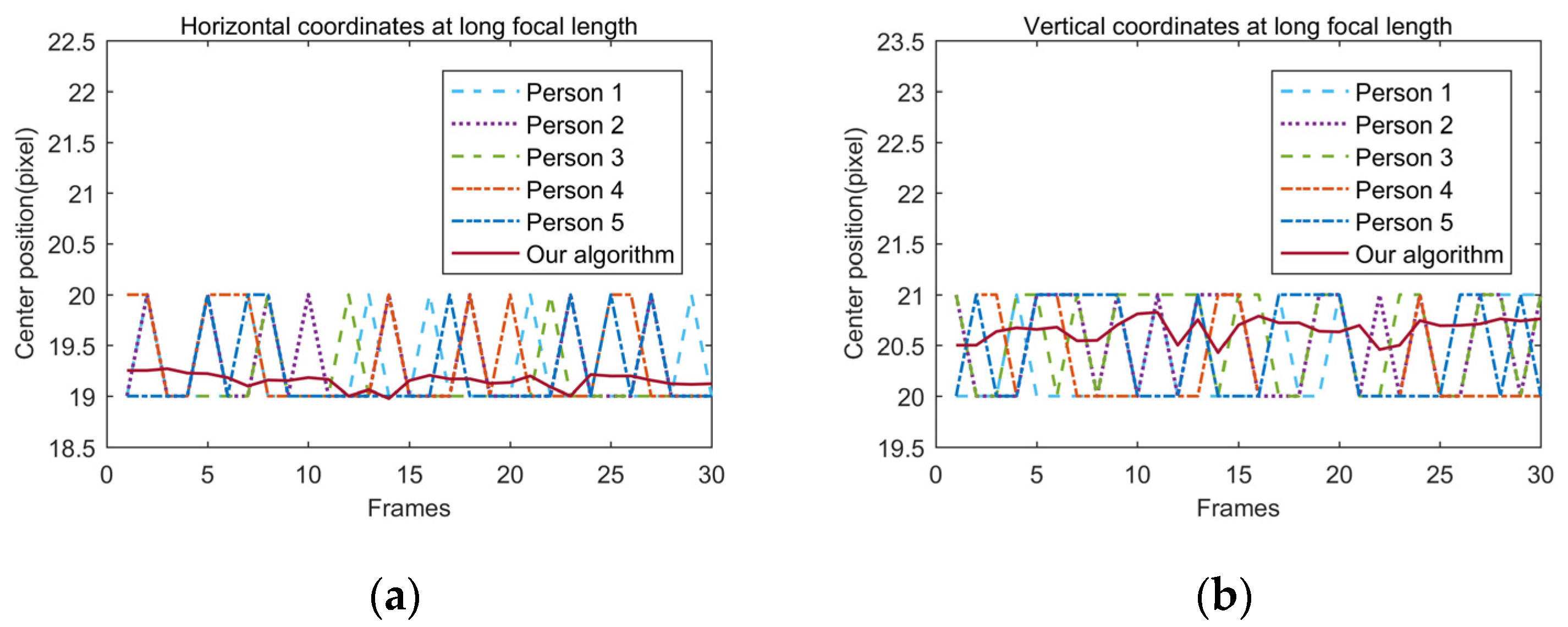
Long focal length	horizontal	19.20	19.27	19.10	19.33	19.23	19.23	19.15
	vertical	20.30	20.53	20.60	20.37	20.47	20.45	20.66

.

At short focal lengths, the spot appears relatively small, facilitating easier localization of its center; observers identify the extraction results as (17, 18). At long focal length, the average center noted by five observers is (19.23, 20.45). In both scenarios, the average center coordinates extracted by our algorithm are closely aligned with the results of human judgment.

Furthermore, we collected real target images as inputs and conducted comparative tests on extraction accuracy and speed against traditional methods. Given that the actual centers of the targets are unknown, our algorithm was employed to process the real images, with the average central coordinates taken as the true centers. Table 3 indicates that the target center coordinate at short focal length is (17.24, 18.44), while at long focal length, it is (19.15, 20.66). These coordinates are derived from the images after extracting the region of interest (ROI) during the preprocessing stage, with each image sized at 40 × 40 pixels. Figure 13 compares the results obtained using different methods on the real images.

The results presented in Figure 13 are generally consistent with the simulation outcomes. In the images captured at short focal lengths, defects in the spot hinder the Hough transform method’s ability to detect the spot effectively. The extraction results in the long focal length images display instability. In contrast, the results obtained using other methods are relatively stable. The circle fitting method demonstrates better performance on real images, because significant noise present in the simulated images adversely affects extraction accuracy. To objectively evaluate the accuracy of our algorithm, we selected average error, maximum error, and time consumption during spot center extraction as evaluation metrics. The comparison between our algorithm and other methods is presented in

Table 4. Comparison of extraction results from different methods in real images.

Image Type	Metric	Hough Transform	Grayscale Centroid	Circle Fitting	Single Dilation (Ours)	Our Algorithm
Short focal length	average error (pixel)	/	0.50	0.49	0.26	0.10
	maximum error (pixel)	/	0.50	1.20	0.30	0.31
	time (ms)	/	15.89	29.28	14.43	16.88
Long focal length	average error (pixel)	1.71	0.48	0.39	0.35	0.11
	maximum error (pixel)	6.75	0.68	0.50	0.50	0.29
	time (ms)	35.53	15.24	32.78	16.48	18.14

.

Table 4 illustrates that the Hough transform method is unable to detect the spot at short focal lengths and demonstrates a relatively large average error at long focal lengths, requiring the longest processing time. The grayscale centroid method yields an average error of approximately 0.5 pixels for both short and long focal lengths. The least squares circle fitting method achieves an average error of no more than 0.5 pixels, indicating the highest accuracy among traditional methods. However, it is susceptible to false detections, as it may identify two spots within a single image. The single dilation method shows an average error of approximately 0.3 pixels, with a maximum error of 0.5 pixels. In contrast, our algorithm achieves an average error of 0.1 pixels at short focal lengths and 0.11 pixels at long focal lengths, with a maximum error of 0.31 pixels, thus significantly outperforming traditional methods. When measuring optical axis parallelism, multiple measurements can be taken and averaged to obtain a final result, effectively reducing measurement error.

In addition, processing speed is a critical indicator for evaluating algorithm performance. Our algorithm requires an average processing time of no more than 20 milliseconds per frame, theoretically supporting a camera operating at 50 FPS. The serial communication frequency of the test camera is 20 Hz. Therefore, the frame rate for image acquisition is set to 20 FPS in the software. The processing time of our algorithm meets the application requirements.

In image processing, the presence of noise significantly impacts algorithm performance. Traditional spot center localization algorithms often experience varying degrees of degradation in detection accuracy due to noise interference. To comprehensively assess the robustness of the proposed algorithm, this study selected Gaussian noise and salt-and-pepper noise as the primary types for sensitivity evaluation. For each type of noise, we generated 30 frames of contaminated test images based on the real images. Subsequently, the proposed algorithm was applied to process both the real and test images, and the processing results were compared to evaluate the algorithm’s resilience to noise interference.

In the experiments, a Gaussian noise model was employed to generate test images by adding noise with a mean of 0 and a standard deviation of $\sigma$ to the original images. Specifically, $\sigma$ values were set at 5, 10, and 15 to create comparable levels of noise interference. Additionally, the proportion of salt-and-pepper noise added was set at 0.01, 0.03, and 0.05.

Table 5. Average error in center extraction of the algorithm under different noise intensities (unit: pixel).

Image Type	Gaussian Noise (Standard Deviation)			Salt-and-Pepper Noise (Probability)
	5	10	15	0.01	0.03	0.05
Short focal length	0.08	0.11	0.21	\	\	\
Long focal length	0.10	0.13	0.14	0.19	0.34	0.80

presents the algorithm’s performance under varying noise intensities.

The results presented in Table 5 indicate that our algorithm maintains a high level of detection accuracy when processing images affected by Gaussian noise. When the standard deviation of the noise reaches 15, the average detection error of the algorithm is 0.21 pixels. In contrast, the detection accuracy significantly decreases for images influenced by salt-and-pepper noise. At short focal lengths, smaller spots can be severely affected by salt-and-pepper noise, potentially leading the algorithm to misidentify the noise as spots, which results in the detection of multiple targets. Based on this analysis, future research will integrate techniques such as median filtering into the algorithm to enhance its resistance to salt-and-pepper noise interference.

4.2.2. Verification of System Function

In prior research, Kong et al. [12] proposed a target center extraction method utilizing the skeleton thinning algorithm for crosshair images captured with a continuous zoom camera. The skeleton thinning algorithm iteratively removes boundary points within the target while preserving junctions, isolated points, and endpoints, until it isolates the core skeleton pixels that represent the image features [25]. However, this method is constrained to pixel-level target center extraction and exhibits a detection error of 1 pixel.

Under the same testing conditions, the target center was extracted using both our algorithm and the skeleton thinning algorithm. Employing the measurement system introduced in this study, we measured the optical axis parallelism of the camera across its entire focal length range. Each method involved three measurements. The results obtained from both methods were visualized based on the software output, as shown in Figure 14.

In Figure 14, the blue curve represents the measurement results obtained using our algorithm while the red curve corresponds to the results derived from the skeleton thinning algorithm. The accuracy of optical axis parallelism measurement is directly dependent on the precision of target center extraction. Traditional methods rely on human visual assessment of the target center’s offset, necessitating a measurement accuracy within an error margin of no more than 1 pixel. The accuracy of our algorithm has been thoroughly validated in Section 4.2.1, thereby ensuring that the resulting optical axis parallelism data are highly reliable. Furthermore, the results displayed in Figure 14 reveal significant fluctuations in the measurements obtained from the skeleton thinning algorithm at short focal lengths, indicating deficiencies in its associated data handling capabilities. In contrast, the results derived from our algorithm exhibit a smoother trend, closely aligning with the actual optical axis parallelism of the camera.

Compared to traditional measurement methods, our system enables continuous and automatic assessment of optical axis parallelism, providing real-time results as measurements are completed. This effectively enhances both measurement accuracy and efficiency. Although the system has achieved its intended functionality, the measurement software presents opportunities for optimization. Currently, the software design is limited to the communication interface standards and resolution for a single type of zoom camera, constraining its applicability. Future work will focus on expanding this capability by integrating relevant parameter configurations into the UI to improve the system’s versatility.

5. Conclusions

To address the limitations of existing methods for measuring optical axis parallelism in continuous zoom cameras, this study developed an online measurement method. First, a spot center positioning method based on morphology techniques was proposed, achieving precise extraction with an average error of 0.13 pixels and a maximum error of 0.31 pixels. Second, measurement software was designed to automatically extract the target center and retrieve focal length data during zooming, outputting the optical axis parallelism across the entire focal length range. Experimental results demonstrate that the proposed system operates stably and accurately measures the optical axis parallelism of continuous zoom cameras in real-time. This capability provides a reliable basis for lens optical axis calibration. Future research will prioritize improving algorithms to mitigate the effects of salt-and-pepper noise as well as enhance software functionalities.

References

- Neil, I.A. Evolution of Zoom Lens Optical Design Technology and Manufacture. Opt. Eng. 2021, 60, 051211. [Google Scholar] [CrossRef]
- Liu, E.; Zheng, Y.; Lin, C.; Zhang, J.; Niu, Y.; Song, L. Research on Distortion Control in Off-Axis Three-Mirror Astronomical Telescope Systems. Photonics 2024, 11, 686. [Google Scholar] [CrossRef]
- Gorshkov, V.A.; Churilin, V.A. Multispectral Apparatus Based on an Off-Axis Mirror Collimator for Monitoring the Quality of Optical Systems. J. Opt. Technol. 2015, 82, 646–648. [Google Scholar] [CrossRef]
- Zhang, Q.; Li, S. Multi-Optical Axis Parallelism Calibration of Space Photoelectric Tracking and Aiming System. Chin. Opt. 2021, 14, 625–633. [Google Scholar] [CrossRef]
- Chen, Z.; Xiao, W.; Ma, D. A Method for Large Distance Multi-Optical Axis Parallelism Online Detection. Acta Opt. Sin. 2017, 37, 112006. [Google Scholar] [CrossRef]
- Jin, W.; Wang, X.; Zhang, Q.; Jiang, Y.; Li, Y.; Fan, F.; Fan, J.; Wang, N. Technical Progress and Its Analysis in Detecting of Multi-Axes Parallelism System. Infrared Laser Eng. 2010, 39, 526–531. [Google Scholar]
- Zhang, L.; Zhao, X. Method for Detecting Coherence of Multiple Optical Axes. In Proceedings of the Fourth Seminar on Novel Optoelectronic Detection Technology and Application, Nanjing, China, 24–26 October 2017. [Google Scholar]
- Luo, M.; Li, S.; Gao, M.; Zhang, Y. Optical Axis Collimation of Biaxial Laser Ceilometer based on CCD. Laser Infrared 2017, 47, 1002–1005. [Google Scholar]
- Zou, H.; Wu, H.; Zhou, L. A Testing Method of Optical Axes Parallelism of Shipboard Photoelectrical Theodolite. In Proceedings of the 8th International Symposium on Advanced Optical Manufacturing and Testing Technology (AOMATT), Suzhou, China, 26–29 April 2016. [Google Scholar]
- Xie, G.; Li, C.; Cai, J. The Test Method of Laser Range Finder Multi-Axis Parallelism. Electron. Test. 2020, 19, 48–51. [Google Scholar]
- Xu, D.; Tang, X.; Fang, G. Method for Calibration of Optical Axis Parallelism Based on Interference Fringes. Acta Opt. Sin. 2020, 40, 129–136. [Google Scholar]
- Kong, F.; Wang, H.; Fang, Y.; Kang, C.; Zhou, F. Measurement Method of Optical Axis Parallelism of Continuous Zoom Camera Based on Skeleton Thinning Algorithm. In Proceedings of the Optical Sensing, Imaging, and Display Technology and Applications, and Biomedical Optics (AOPC), Beijing, China, 25–27 July 2023. [Google Scholar]
- Yao, Z.; Yi, W. Curvature Aided Hough Transform for Circle Detection. Expert Syst. Appl. 2016, 51, 26–33. [Google Scholar] [CrossRef]
- Li, Z.; Liao, L. Bright Field Droplet Image Recognition Based on Fast Hough Circle Detection Algorithm. In Proceedings of the 2022 14th International Conference on Computer Research and Development (ICCRD), Shenzhen, China, 7–9 January 2022. [Google Scholar]
- Yao, R.; Wang, B.; Hu, M.; Hua, D.; Wu, L.; Lu, H.; Liu, X. A Method for Extracting a Laser Center Line Based on an Improved Grayscale Center of Gravity Method: Application on the 3D Reconstruction of Battery Film Defects. Appl. Sci. 2023, 13, 9831. [Google Scholar] [CrossRef]
- Wang, J.; Wu, J.; Jiao, X.; Ding, Y. Research on the Center Extraction Algorithm of Structured Light Fringe Based on an Improved Gray Gravity Center Method. J. Intell. Syst. 2023, 32, 20220195. [Google Scholar] [CrossRef]
- Chernov, N.; Lesort, C. Least Squares Fitting of Circles. J. Math. Imaging Vis. 2005, 23, 239–252. [Google Scholar] [CrossRef]
- Yatabe, K.; Ishikawa, K.; Oikawa, Y. Simple, Flexible, and Accurate Phase Retrieval Method for Generalized Phase-Shifting Interferometry. J. Opt. Soc. Am. A 2016, 34, 87–96. [Google Scholar] [CrossRef]
- Klančar, G.; Zdešar, A.; Krishnan, M. Robot Navigation Based on Potential Field and Gradient Obtained by Bilinear Interpolation and a Grid-Based Search. Sensors 2022, 22, 3295. [Google Scholar] [CrossRef] [PubMed]
- Xu, X.; Xu, S.; Jin, L.; Song, E. Characteristic Analysis of Otsu Threshold and Its Applications. Pattern Recognit. Lett. 2011, 32, 956–961. [Google Scholar] [CrossRef]
- Said, K.A.M.; Jambek, A.B.; Sulaiman, N. A Study of Image Processing Using Morphological Opening and Closing Processes. Int. J. Control Theory Appl. 2016, 9, 15–21. [Google Scholar]
- Sekehravani, E.A.; Babulak, E.; Masoodi, M. Implementing Canny Edge Detection Algorithm for Noisy Image. Bull. Electr. Eng. Inform. 2020, 9, 1404–1410. [Google Scholar] [CrossRef]
- Suzuki, S. Topological Structural Analysis of Digitized Binary Images by Border Following. Comput. Vis. Graph. Image Process. 1985, 30, 32–46. [Google Scholar] [CrossRef]
- Hu, F.; Yan, Y.; Huang, Y. Research on Simulation Monitoring System of 828D Machining Center Based on QT. Sci. J. Intell. Syst. Res. Vol. 2021, 3, 3. [Google Scholar]
- Ma, J.; Ren, X.; Tsviatkou, V.Y.; Kanapelka, V.K. A Novel Fully Parallel Skeletonization Algorithm. Pattern Anal. Appl. 2022, 25, 169–188. [Google Scholar] [CrossRef]