Article

Feature Vector Effectiveness Evaluation for Pattern Selection in Computational Lithography

1
State Key Laboratory of Intelligent Manufacturing Equipment and Technology, Huazhong University of Science and Technology, Wuhan 430074, China
2
Optics Valley Laboratory, Wuhan 430074, China
*
Authors to whom correspondence should be addressed.
These authors contributed equally to this work.
Photonics 2024, 11(10), 990; https://doi.org/10.3390/photonics11100990
Submission received: 24 September 2024 / Revised: 18 October 2024 / Accepted: 19 October 2024 / Published: 21 October 2024

Abstract

:
Pattern selection is crucial for optimizing the calibration process of optical proximity correction (OPC) models in computational lithography. However, it remains a challenge to achieve a balance between representative coverage and computational efficiency. This work presents a comprehensive evaluation of the feature vectors’ (FVs’) effectiveness in pattern selection for OPC model calibration, leveraging key performance indicators (KPIs) based on Kullback–Leibler divergence and distance ranking. Through the construction of autoencoder-based FVs and fast Fourier transform (FFT)-based FVs, we compare their efficacy in capturing critical pattern features. Validation experimental results indicate that autoencoder-based FVs, particularly augmented with the lithography domain knowledge, outperform FFT-based counterparts in identifying anomalies and enhancing lithography model performance. These results also underscore the importance of adaptive pattern representation methods in calibrating the OPC model with evolving complexities.

1. Introduction

It is well-known that the optical proximity correction (OPC) model is indispensable for ensuring design-to-wafer fidelity in advanced lithography [1]. An essential aspect of constructing a satisfactory parametric OPC model involves ensuring the presence of sufficient and relevant test pattern representatives in the calibration set. The quality of selected pattern samples for the test pattern representatives has a direct influence on the accuracy of the parametric OPC model [1,2]. Usually, the higher the quality of the pattern samples, the higher the accuracy of the OPC model fitted thereby. Also, there is a positive correlation between the OPC model’s accuracy and the sample set’s coverage. When the number of pattern samples is insufficient, the coverage of the pattern set is often low, and the OPC model is prone to overfitting problems. Moreover, if the parameters of the OPC model are not fully trained, then the model’s prediction ability will be affected. Conversely, when the number of selected samples is too large, overloading the OPC model training causes the model fitting workload to increase significantly. Therefore, it is a great challenge to quickly select representative pattern samples to balance the pattern coverage, sample amount, runtime, and resource.
In recent decades, numerous approaches have been proposed to optimize the pattern coverage space to achieve a reliable OPC model with high accuracy and predictability [1,2]. Using the feature vectors (FV) extracted from aerial images, crucial optical and geometrical details can be retained efficiently. It also enables the differentiation of various patterns by analyzing the corresponding FV distribution within the feature space [3]. Meanwhile, to assess the pattern coverage index for a given pattern set, a typical approach focuses on computing the feature vector-based coverage index by comparing representative patterns against the selected patterns [4]. A simulation-based alternative metric could also be devised according to the model‘s error severity estimation, which enables guiding the incremental pattern selection for the calibration pattern set. This strategy serves to enhance the accuracy of the OPC model while expediting the calibration process [4]. Moreover, some research has demonstrated the efficacy of machine learning techniques in selecting essential and representative patterns for calibrating the OPC model [3,4]. However, as lithography advancements continue to drive pattern complexity, the need for adaptive and efficient pattern representation methods becomes paramount.
In the semiconductor industry, the design target pattern layout is usually the combination of limited unit cells, leading to the intrinsic dimensionality of design target pattern images being even smaller than natural images [5]. However, the data distribution in the pattern pool is highly unbalanced. Some patterns lying in memory cells can appear millions of times across the entire design layout, while some specific patterns at the cell boundary only appear once in the whole pattern pool. Also, some patterns will derive a considerable amount of high similarity patterns due to retargeting or variation of surrounding features, while some patterns show significant geometry differences from all others. Thus, a highly efficient pattern representation method is required to simultaneously capture the critical features of patterns and adapt to the data distribution to avoid unbalanced feature extraction.
The manifold hypothesis asserts that high-dimensional data lies on or near a low-dimensional manifold within the high-dimensional space. And the low-dimensional manifold can also significantly suppress the curse of dimensionality, leading to sharp boundaries in further clustering usage and outlier detection [6,7,8,9]. A well-constructed autoencoder (AE) network can capture the non-linear relationships between the input pattern images. Thus, it can use a low-dimensional manifold to represent the raw pattern space. The multiple-layer machine learning network empowers an autoencoder to learn a hierarchical representation for the input data. This highly efficient feature encoding allows a much lower feature dimension while keeping the primary critical pattern information [4]. In a previous work [4], AE exhibited superior performance in pattern selection applications and enhanced final model accuracy. However, the proof data focused on the indirect model performance of the overall pattern selection. The direct validation of its feature extraction efficacy remains unestablished. Considering that AE is self-adaptive to integrating various types of domain knowledge through additional constraints, fine-tuning the network is promising to enhance the efficacy of the pattern selection. Thus, a direct and comprehensive evaluation of their effectiveness is essential for guiding future enhancements of the AE network.
In this work, we first collect a dataset with diverse pattern designs and limited critical patterns for the OPC model calibration. Two key performance indicators (KPI), namely, the distance ranking and the Kullback–Leibler (KL) divergence, are constructed to realize the direct evaluation of the effectiveness of the FV-based pattern selection. Then, the KPI-based effectiveness estimation and comparison were carried out on the FFT-based FV, unsupervised AE-based FV, and improved AE-based FV, which revealed the efficacy of the AE-based feature vector in improving pattern coverage for the OPC model calibration. Moreover, tuning the AE network and loss function facilitates the improvement of the final pattern selection/coverage strategy.

2. Materials and Methods

2.1. Two KPIs for Feature Vector Effectiveness Evaluation

The objective of pattern selection is to achieve a sub-set from the entire dataset and approach a minimum data bias to the whole dataset. When a typical sub-set is used for the OPC model training, the data distribution in this sub-set will induce minimum data bias trend and avoid additional over-fitting. A representative pattern selection flow will convert patterns into FVs and apply distance-based clustering or ranking methods to construct sub-sets [10,11,12,13]. In the previous work [4,6,14,15], we found that the majority of data bias for the sub-set comes from two aspects, namely, the selection method and the FV effectiveness.
The selection method will dramatically affect the data distribution of the sub-set. For example, if the random selection is used and the sub-set population is large enough, the sub-set usually tends to pick more elements from regions with high density in the FV space. Then, elements with higher probability density in the entire set will still show higher probability in the sub-set. However, in industry practical usage, the initial set is usually a mixed dataset from multiple data sources during the industry’s practical usage, leading to the pattern distribution being initially far from ideal and homogeneous. Correspondingly, the random selection will thoroughly inherit this biased distribution, leading to poor selection results. With a well-designed selection methodology, the sub-set can leverage data diversity more by adding the sample ratio in low-probability regions to avoid missing critical outliers [4,6,14].
Meanwhile, the FV effectiveness will also significantly affect any well-designed FV-based selection method [15]. Contrary to the random selection, the FV-based selection assumes the FV can help adjust the sample rate based on lithography domain knowledge. An effective FV should keep critical information of the raw image and drop redundant information with an un-close correlation to the downstream OPC tasks. Thus, by evaluating the FV similarity, the sample rate among similar patterns can be reduced to expand pattern coverage. Euclidean distance in feature space is widely used in similarity judgment, clustering, or ranking solutions. However, if the FV fails to capture critical features or contains too many redundancies, it can lead to severe multicollinearity. In such scenarios, the Euclidean distance will not be able to represent the similarity or domain overlap situations between two datasets.
Based on the above considerations, we use two KPIs to quantify the FV effectiveness. The first KPI is distance ranking, which is an intuitive method in practical usage [10,14,16,17]. Assume we already have a sub-set SC used for lithography model calibration. We can examine the minimum Euclidean distance from every pattern in the validation set SV to the sub-set SC, sort the distances from small to large, and achieve the ranking REuc(x) with xSV. After the model calibration, when we apply the model on all validation data to obtain the model error, we discover the outlier set SO and its corresponding ranking REuc(x) with xSO. If the FV effectiveness is high, the outliers should have a much larger distance than the normal patterns. Thus, the ranking of outliers should exhibit a small value in both average ranking and standard deviation. The distance calculation may not be limited to Euclidean but can be adjusted flexibly in clustering processes.
The second KPI is KL divergence, also known as Kullback–Leibler divergence, which is a type of statistical distance measuring how one probability distribution diverges from a second reference probability distribution [18]. It originates from information theory to represent relative entropy and has been widely used in various areas to quantify the distance between two distributions. The KL divergence can quantify the gap between the feature space distribution of two certain datasets. When two datasets come from the same probability distribution, their KL divergence should approach 0. With the growth of the distribution disagreements, the KL divergence will also enlarge. Since outliers differ dramatically from calibration patterns in the lithography domain, an effective FV should exhibit a large gap between the outliers and the calibration patterns and, thus, a considerable KL divergence between them.
For continuous probability distributions P(x) and Q(x) defined on the same sample space, we can define the KL divergence from Q(x) to P(x) as [18]:
D K L P Q = P x log P x Q x d x
However, in most cases, the actual probability density function is rarely known. The critical problem is to estimate the entropy and divergence of related distributions only from a finite number of samples. One potential solution is k-nearest-neighbor-based estimators to approximate the probability density function under the assumption of multi-dimensional ε-ball [19]. Compared to the a priori kernel density estimator (KDE), it is computationally more efficient in high dimensions [20]. Assume the distance from Xi to its k-nearest-neighbor in {Yi} is denoted by vk(i), and one d-dimensional open Euclidean ball is centered at x with radius ρ, then the estimator for KL divergence is:
D n , m p q = d n i = 1 n log v k i ρ k i + log m n 1
where n and m are the size of the d-dimensional samples {X1, X2, X3, …, Xn} and {Y1, Y2, Y3, …, Ym} drawn independently from P(x) and Q(x), respectively.
When KL divergence is applied on some FVs, with P(x) being the KDE of the calibration set and Q(x) being the KDE of outliers, the KL divergence should show a positive correlation to FV effectiveness.

2.2. Experiment Case

In order to evaluate the FV effectiveness via the two KPIs, a practical pattern set with clear outliers is needed. In this work, we used a contact hole layout of a typical memory device to construct the pattern set. The lithography process was performed with an ASML immersion deep ultraviolet (DUV) scanner with numerical aperture (NA) = 1.3 from Netherlands. And the corresponding mask was OPC-ed by a production-level baseline lithography model.
For a typical production-level lithography model, the model quality is good enough for most patterns. The lithography model is calibrated with physically driven terms, enabling good generalization ability. Thus, patterns with dramatically different design shapes can usually cover each other in the lithography domain. Only the outliers with significant model errors cannot be clearly covered by the majority of patterns.
The whole pattern set was picked from this full-chip layout via mixed selection methods, including random selection, diversity-based selection [4], and simulation property-based selection. This mixed selection aims to construct a dataset that is not severely influenced by pattern population. Since different selection strategies have different focuses, we use the mixed selection method to make the final selection diverse enough to cover as much pattern sensitivity as possible.
The first step before each detailed selection is a pattern collection from a full-chip layout. This collection systematically scans a complete chip layout and identifies all the geometrically unique patterns. The “unique” here means within a certain radius, the geometry configuration of one pattern will not be the same as any other pattern. In DUV lithography model calibration, only neighboring contents within a certain radius will influence lithography model prediction. Thus, this radius is used as a radius in pattern definition. Usually, one pattern can be repeated multiple times across a full-chip layout in the design stage. And these repeating instances will exhibit almost the same lithography behavior. As shown in Figure 1, this pattern collection will first break the layout into patterns that cover the full area with circuit designs, the red cross in subfigure b indicates pattern center and the red box indicates pattern boundary. Then, a pattern-matching process will remove repeating patterns and only keep unique patterns. This pattern collection strategy can trim the repeating patterns and focus only on unique patterns exhibiting different lithography behaviors.
After the pattern collection, the unique pattern set amount can still easily reach the million level from a full-chip layout. However, a typical scanning electron microscope (SEM) metrology verification process can only afford a thousand-level pattern input. We then further down-selected to construct a fair dataset that covers the majority of pattern designs while not markedly affecting the data distribution of the whole set. The random selection aims to achieve a direct fair-down selection from the initial unique pattern set. We used multiple rounds of random selection to pick 2000 patterns as the basis of the pattern set.
Since the sample ratio is low, pure random selection will still miss many representative patterns in the low-probability region of the design space. We use additional selections to pick more patterns from different aspects. Sun et al. demonstrated that diversity-based selection can capture diverse patterns via the feature vectors [4]. Different feature vectors project the pattern set to a specific feature space and identify pattern design trends/clusters. We also applied multiple rounds of diverse-based selection with various-type feature vectors to select 1400 patterns to supplement the pattern set.
Finally, 50 patterns were added to the pattern set via the simulated process variation sensitivity with the baseline lithography model. We simulated the process variation sensitivity for all unique patterns and picked out the top-ranking ones as high-risk candidates. The quality of overall 3450 patterns was estimated using their SEM metrology data, and about 25 patterns were dropped due to the low SEM image quality. For every pattern with good SEM image quality, multiple gauges were placed to extract the wafer critical dimension (CD) using a Hitachi CD-SEM machine from Japan. The Critical Dimension is the smallest feature size on a chip during semiconductor manufacturing. In the following model calibration and model check process, the maximum absolute model error under one pattern will be marked as the model error of this pattern.

2.3. Outlier Identification

Outliers are critical for evaluating the FVs’ effectiveness. When the lithography model exhibits good generalization ability, all patterns show low model error, which makes it hard to distinguish outliers. We intentionally reduced the calibration set volume to calibrate a new lithography model with relatively poorer generalization ability. The outlier patterns that appeared with more significant model errors can then be used as a probe to evaluate the FV effectiveness. We used 1000 patterns to construct a new calibration set, in which every pattern is randomly selected from a complete set with 3425 patterns. Model error (+/− 10 nm) is chosen as outlier criteria since it is a typical model error range in the current tech node considering SEM machine metrology error, SEM image quality, and OPC model fitting power.
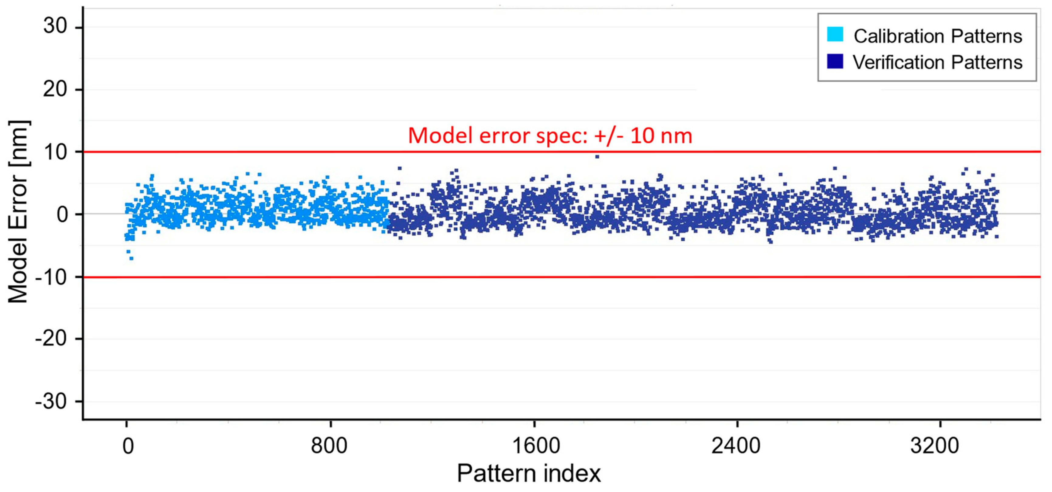
As shown in Figure 2 and Table 1, the new model was calibrated by 1000 selected patterns (with 2000 gauges), the model root mean square (RMS) of the calibration pattern set was 1.62 nm and the model error range (the range between the maximum model error and minimum model error) of calibration pattern set was at 7.94 nm; all patterns met the model error spec for tape out (in +/− 10 nm). However, when the new model was applied to the remaining 2425 patterns, 30 model error outliers as shown in red cycle (with model error > 10 nm or model error < −10 nm) were found. The outliers potentially come from 3 aspects, while only one aspect is suitable for the evaluation of the FV effectiveness.
(a)
The outliers show a significant gap in the lithography domain to the calibration set, and thus cannot be generalized by the baseline model.
(b)
Special lithography effects exist in the outliers, and the lithography model lacks the fitting power to fit on these outliers.
(c)
The SEM metrology quality is poor on the outliers, and the “wafer CD” collected for the calibration/verification is not the actual wafer CD.
We further performed another process to confirm the source of the outliers. We added the 30 outlier patterns into the calibration set and re-calibrated the model with 1030 patterns (with 2060 gauges). The updated calibration and verification results are shown in Figure 3 and Table 2. All calibration and verification patterns met the model error specifications. This means that the root cause of the 30 model error outliers is the aspect, and the outliers are dramatically different from the 1000 calibration patterns in the lithography domain. After adding them to the calibration, they all met the model error specification with negligible trade-offs on other patterns.
Based on such confirmation, we can use these 30 outlier patterns as an indicator to benchmark the effectiveness across different FVs directly. An effective FV should show significant discrimination between the outlier and majority patterns in the FV space.

2.4. Three Feature Vector Generation Methods

To compare the effectiveness across different FVs, we prepared three types of FVs. The first one is the FFT-based FV. The FFT kernel functions are naturally orthogonal and thus show little feature redundancy to benefit further distance calculation. Also, the optical part of the lithography process can be regarded as an Abbe imaging process. The diffraction orders of a pattern in the source panel are naturally the FFT feature component of the mask design. The interaction between the source illumination and the FFT components of the pattern will significantly affect the imaging quality and, thus, the lithography model calibration status [21,22]. The FFT-based FV is widely used in lithography-related machine learning applications, and thus, we use it as the baseline FV in pattern selection solutions [23,24].
In industry usage, one not-bad option is constructing a feature vector based on empirical knowledge. OPC engineers construct feature vectors using clear corresponding physical properties. Although some important components will definitely be missed, it offers users a tuning knob to embed empirical knowledge into the feature vector. AE combines the benefits of the above two solutions. Its network-enabled encoded FV carries most of the input image information, while the flexibility in loss function allows end users to embed empirical knowledge into the feature vector.
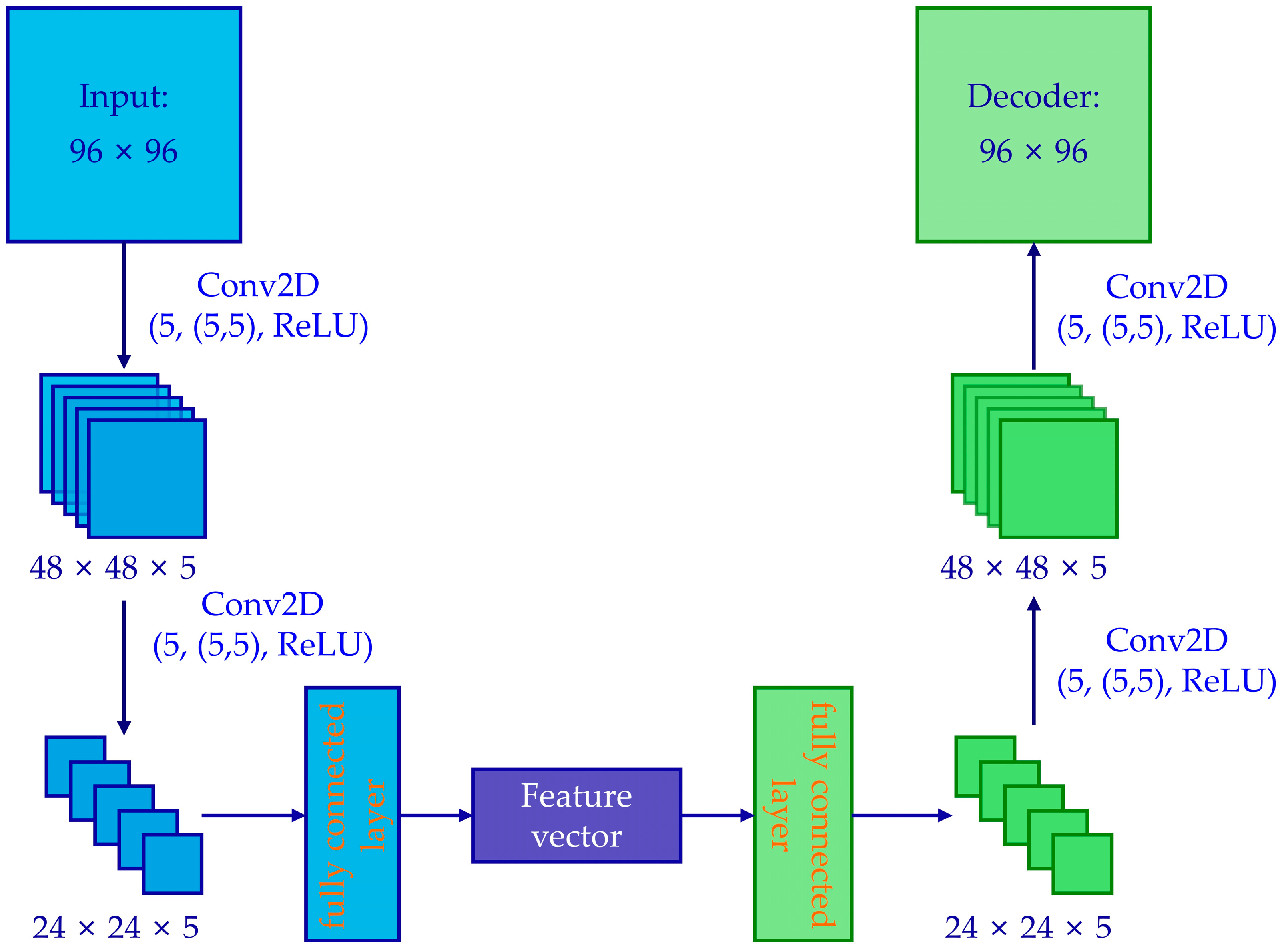
Thus, the second FV is an unsupervised AE-based FV with basic mean square error (MSE) loss used between the input and output images. In contrast to the FFT-based FV, the dimensions of the AE features are learned by a typical deep-learning network and are not orthogonal to each other. As shown in Figure 4, the AE network is constructed by symmetrical encoder and decoder parts. The convolution layer kernel size and count are tunable to adjust the encoder dimension. The MSE loss forces the network to extract critical features of input images that can help restore an image at the network’s end with pixel-level information consolidated [7,8,9]. By reducing FV dimensionality, redundant features can be dropped during the training progress, leading to higher discrimination ability in the AE-based feature space but sacrificing the MSE loss and generalization ability.
The aerial images calculated by the lithography model are used as the training input for the AE network. The lithography model uses physical terms to construct a compact mathematical model of the whole lithography process. The aerial images are the intermediate result, including the interaction of illumination light through scanner optics, mask transmission, and the multiple-layer resist films [25,26]. The aerial images are already very similar to the final simulated pattern shape. Thus, they contain the geometry characters of the pattern design. Moreover, the aerial images take almost all optical effects in the lithography process, containing much more lithography domain knowledge than pure design shapes. The pixel size of aerial images is 14 nm in the current case, and the image size is 96 pixels, corresponding to the typical model ambit of DUV models.
This AE network will be capable of capturing the non-linear relationships embedded in the aerial images that are closely related to lithography model calibration. To avoid overfitting, 80% of the patterns were randomly selected for the model training of the AE network, and the other 20% of the patterns were used for verification. The MSE loss function of the AE network with different dimensions is shown in Table 3. The verification loss values are comparable to training loss values in the same dimension, which means no overfitting for the AE networks. Moreover, the loss value increases after decreasing the feature vector dimension. The phenomenon was expected because a lower dimension meant less information (including information from redundant features) retained in the feature vector without loss of generality.
The third FV is an improved AE-based FV with more constraints imposed on the aerial contour locations. Generic AE FV is selected to demonstrate its capacity with FFT FV while the improved AE FV is used to demonstrate the benefit from empirical knowledge. Even though information loss cannot be neglected in the AE encoding process, we still believe that the remaining critical features can better represent patterns needed to calibrate the lithography model. Also, the training loss can be designed to concentrate more on the specific domain due to the machine learning network’s intrinsic capacity. And specific information that is well acknowledged as less critical is sacrificed [27]. In the lithography process, it is well addressed that the image slope significantly affects the imaging quality. Thus, the improved AE network can be tuned to extract more slope information by adding MSE loss between the image slopes of the input and output images to the total loss function. Following the same strategy of the improved AE network with MSE loss, the training loss for 80% of training patterns and verification loss for the other 20% of patterns are shown in Table 4.

3. Results

These three FV generation methods are applied to the whole pattern pool to obtain the corresponding FV for each pattern. FV dimension is a critical parameter in pattern selection usages. The higher the FV dimension, the more occupied disk space, and the longer runtime. The smaller FV dimension will compress too much from the original input images and lose critical information. Five-dimension values are used in this work to match actual application usages: 49, 100, 196, 400, and 729.
Figure 5 shows the KPI comparison across all three FVs. The box plot shows the distribution of the ranking result, with box length indicating the ranking gap from the 75th percentile to the 25th percentile and orange line indicating the median value. The whisper indicates the full range of ranking gaps, and the circle shows limited aberrations with dramatically different rankings. The smaller ranking number refers to the outliers with a more considerable distance to calibration patterns.
As For the FVs with dimension 729, the curse of dimensionality damaged the discrimination capacity of the AE-based FV. Most outliers failed to separate from normal patterns. However, distance-based FV solutions can hardly hit actual issue patterns if the objective is an outlier discovery. The KL divergence of three FVs is comparable with a small value close to zero, showing poor discrimination capability.
When the FV dimension is reduced, the FFT-based FV shows stable KPIs in both ranking and KL divergence aspects. It indicates that the high-frequency components after the FFT are not critical enough to describe the differences between calibration and outlier patterns in this case. On the contrary, the AE-based FV shows much better behavior than the FFT-based FV. The ranking box and whisper ranges are all reduced and agree well with the KL divergence. The improved AE-based FV shows the best result, accompanied by the majority of outliers ranking in the top 100, and the KL divergence is also much more significant than basic AE-based and FFT-based FVs. It also confirmed that adding more domain knowledge into the AE network training can effectively benefit the FV effectiveness in pattern selection usage for lithography model calibration.
In pattern selection processes, various strategies can be applied to pick representative patterns. When the probability distribution of critical outliers fully overlaps with majority patterns, the KL divergence will be zero and no strategy can distinguish outliers by feature vectors. With increasing KL divergence, the separation of outliers and majority patterns will increase, enabling selection methods to highlight outliers without picking too many majority patterns.
The distance ranking itself can be used as a straightforward selection strategy by directly picking top N ranking patterns as a selection result. In the current case, when KL divergence is 0.14 (AE FV in dimension 49), the top 430 patterns should be picked to cover 90% outliers. While when KL divergence increased to 0.91 (improved AE FV in dimension 49), only the top 60 patterns needed to cover 90% of outliers.
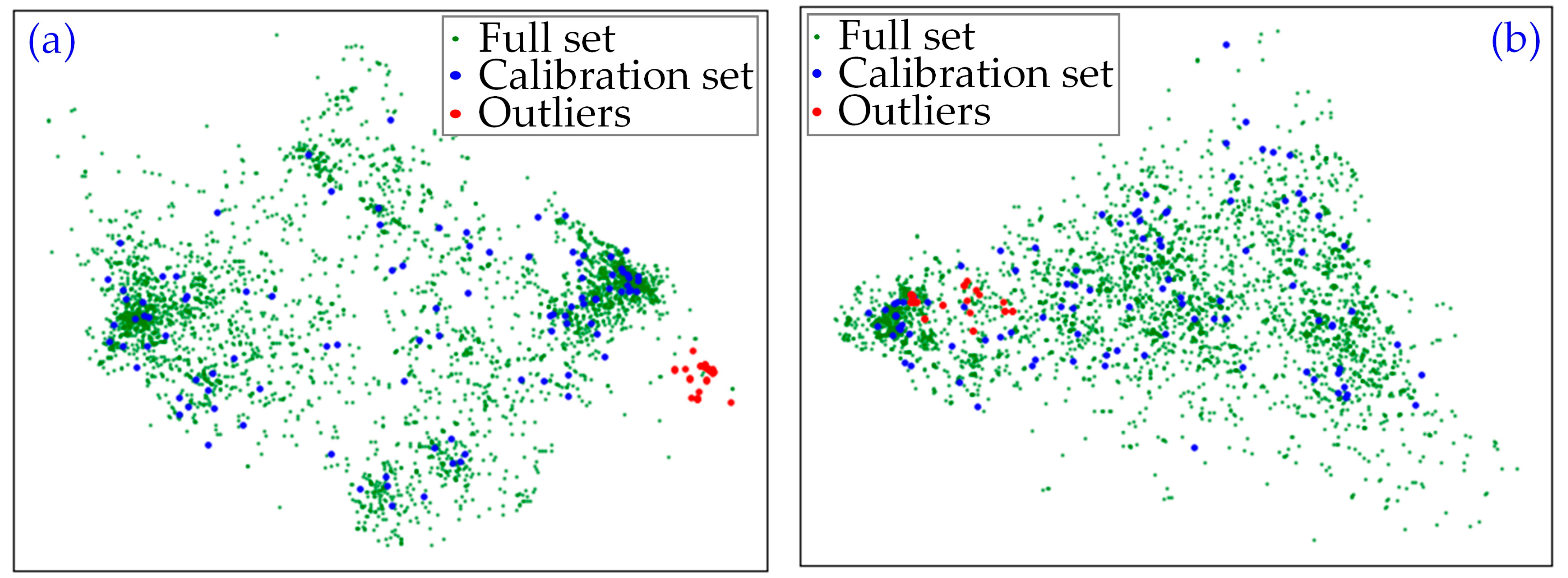
When analyzing high-dimensional data, Principal Component Analysis (PCA) is a widely used tool to compress data to low dimension. Although PCA dropped a lot of information, and low-dimension distance cannot fully reveal the original FV space distribution, PCA can still provide a qualitative visualization. Since we observed the improved AE showing much better effectiveness than the basic AE in both KPI comparisons, we further performed PCA-based 2D visualization between the improved and basic AE FVs under dimension 49 in Figure 6. The PCA visualization indicates that the improved AE has a much better separation between the outliers and the calibration set.

4. Conclusions

We designed an experiment to directly evaluate the FV effectiveness in pattern selection usages for lithography model calibration. Two KPIs were constructed to quantify the FV effectiveness. Both KPIs confirmed that AE-based FV is more effective than FFT-based FV in extracting critical pattern features with considerable sensitivity to the lithography model performance. Moreover, the autoencoder is highly effective in adopting domain knowledge into loss construction and further improves the FV’s effectiveness in identifying anomalies from a large pattern pool.

Author Contributions

Conceptualization, Y.F., J.L., H.J. and S.L.; methodology, Y.F., J.L., H.J. and S.L.; formal analysis, Y.F. and J.L.; Software, Y.F.; Data curation, Y.F. and J.L.; Investigation, Y.F., J.L., H.J. and S.L.; Visualization, Y.F. and J.L.; Validation, Y.F., J.L. and S.L.; resources, Y.F, J.L., H.J. and S.L.; writing—original draft preparation, Y.F. and J.L.; writing—reviewing and editing, Y.F., J.L., H.J. and S.L.; funding acquisition, J.L., H.J. and S.L.; supervision, S.L.; project administration, S.L. All authors have read and agreed to the published version of the manuscript.

Funding

This research was funded by the National Natural Science Foundation of China (Grant Nos. 52130504, 52305577, and 52205592), the Key Research and Development Plan of Hubei Province (Grant No. 2022BAA013), the Major Program (JD) of Hubei Province (Grant No. 2023BAA008-2), the Innovation Project of Optics Valley Laboratory (Grant No. OVL2023PY003), the Postdoctoral Fellowship Program (Grade B) of China Postdoctoral Science Foundation (Grant No. GZB20230244), and the Fellowship from the China Postdoctoral Science Foundation (2024M750995).

Institutional Review Board Statement

Not applicable.

Informed Consent Statement

Not applicable.

Data Availability Statement

Data will be made available on request.

Acknowledgments

The authors would like to thank the technical support from the Experiment Center for Advanced Manufacturing and Technology in the School of Mechanical Science & Engineering of HUST.

Conflicts of Interest

The authors declare no conflicts of interest.

References

  1. De Bisschop, P. How to make lithography patterns print: The role of OPC and pattern layout. Adv. Opt. Technol. 2015, 4, 253–284. [Google Scholar] [CrossRef]
  2. Schlief, R.E. Effect of data selection and noise on goodness of OPC model fit. In Optical Microlithography XVIII, Proceedings of the Microlithography 2005, San Jose, CA, USA, 27 February–4 March 2005; SPIE: Bellingham, WA, USA, 2005; Volume 5754, p. 5754. [Google Scholar]
  3. Vengertsev, D.; Kim, K.; Yang, S.H.; Shim, S.; Moon, S.; Shamsuarov, A.; Lee, S.; Choi, S.W.; Choi, J.; Kang, H.K. The new test pattern selection method for OPC model calibration, based on the process of clustering in a hybrid space. In Photomask Technology 2012, Proceedings of the SPIE Photomask Technology, Monterey, CA, USA, 11–13 September 2012; SPIE: Bellingham, WA, USA, 2012; Volume 8522, pp. 387–394. [Google Scholar]
  4. Sun, R.C.; Kang, D.K.; Jia, C.; Liu, M.; Shao, D.B.; Kim, Y.S.; Shin, J.; Simmons, M.; Zhao, Q.; Feng, M.; et al. Enhancing model accuracy and calibration efficiency with image-based pattern selection using machine learning techniques. In Optical Microlithography XXXIV, Proceedings of the SPIE Advanced Lithography, Online Only, CA, USA, 22–27 February 2021; SPIE: Bellingham, WA, USA, 2021; Volume 11613, pp. 214–222. [Google Scholar]
  5. Zhang, W.; Pang, B.; Ma, Y.; Li, X.; Bai, F.; Wang, Y. Modeling sampling strategy optimization by machine learning based analysis. In Proceedings of the 2021 International Workshop on Advanced Patterning Solutions (IWAPS), Foshan, China, 12–13 December 2021; IEEE: New York, NY, USA, 2021; pp. 1–4. [Google Scholar]
  6. Feng, Y.; Song, Z.; Liu, J.; Li, Z.; Yang, F.; Jiang, H.; Liu, S. Layout pattern analysis and coverage evaluation in computational lithography. Opt. Express 2023, 31, 8897–8913. [Google Scholar] [CrossRef] [PubMed]
  7. Zhang, L.; Zhang, Q.; Du, B.; You, J.; Tao, D. Adaptive manifold regularized matrix factorization for data clustering. In Proceedings of the International Joint Conference on Artificial Intelligence, Melbourne, Australia, 19–25 August 2017; pp. 3399–3405. [Google Scholar]
  8. Ansuini, A.; Laio, A.; Macke, J.H.; Zoccolan, D. Intrinsic dimension of data representations in deep neural networks. Adv. Neural Inf. Process. Syst. 2019, 33, 6111–6122. [Google Scholar]
  9. Gong, S.; Boddeti, V.N.; Jain, A.K. On the intrinsic dimensionality of image representations. In Proceedings of the 2019 IEEE CVF Conference on Computer Vision and Pattern Recognition (CVPR), Long Beach, CA, USA, 15–20 June 2019; pp. 3982–3991. [Google Scholar]
  10. Kohli, K.K.; Jobes, M.; Graur, I. Automated detection and classification of printing sub-resolution assist features using machine learning algorithms. In Optical Microlithography XXX, Proceedings of the SPIE Advanced Lithography, San Jose, CA, USA, 26 February–2 March 2017; SPIE: Bellingham, WA, USA, 2017; Volume 10147, pp. 176–182. [Google Scholar]
  11. Ganin, Y.; Lempitsky, V. Unsupervised domain adaptation by backpropagation. In Proceedings of the International Conference on Machine Learning, Lile, France, 6–11 July 2015; PMLR: Westminster, UK, 2015; pp. 1180–1189. [Google Scholar]
  12. Vazquez, D.; Lopez, A.M.; Marin, J.; Ponsa, D.; Geronimo, D. Virtual and real world adaptation for pedestrian detection. IEEE Trans. Pattern Anal. Mach. Intell. 2013, 36, 797–809. [Google Scholar] [CrossRef] [PubMed]
  13. Zeiler, M.D.; Fergus, R. Visualizing and understanding convolutional networks. In Proceedings of the Computer Vision–ECCV 2014: 13th European Conference, Zurich, Switzerland, 6–12 September 2014; Springer International Publishing: Cham, Switzerland, 2014; pp. 818–833. [Google Scholar]
  14. Bae, K.; Kim, T.; Lee, S.; Kim, B.; Jeong, S.; Tang, J.; Zhao, Q.; Zhao, Y.; Choi, C.-I.; Liang, J.; et al. Advanced Pattern Selection and Coverage Check for Computational Lithography. In Advances in Patterning Materials and Processes XLI, Proceedings of the SPIE Advanced Lithography + Patterning, San Jose, CA, USA, 25 February–1 March 2024; SPIE: Bellingham, WA, USA, 2024. [Google Scholar]
  15. Ding, D.; Wu, X.; Ghosh, J.; Pan, D.Z. Machine learning based lithographic hotspot detection with critical-feature extraction and classification. In Proceedings of the 2009 IEEE International Conference on IC Design and Technology, Austin, TX, USA, 18–20 May 2009; IEEE: New York, NY, USA, 2009; pp. 219–222. [Google Scholar]
  16. Yang, F.; Sinha, S.; Chiang, C.C.; Zeng, X.; Zhou, D. Improved tangent space-based distance metric for lithographic hotspot classification. IEEE Trans. Comput. -Aided Des. Integr. Circuits Syst. 2016, 36, 1545–1556. [Google Scholar] [CrossRef]
  17. Cavalcanti, G.D.; Soares, R.J. Ranking-based instance selection for pattern classification. Expert Syst. Appl. 2020, 150, 113269. [Google Scholar] [CrossRef]
  18. Kullback, S.; Leibler, R.A. On information and sufficiency. Ann. Math. Stat. 1951, 22, 79–86. [Google Scholar] [CrossRef]
  19. Wang, Q.; Kulkarni, S.R.; Verdú, S. Divergence estimation for multidimensional densities via k-Nearest-Neighbor distances. IEEE Trans. Inf. Theory 2009, 55, 2392–2405. [Google Scholar] [CrossRef]
  20. Lombardi, D.; Pant, S. Nonparametric k-nearest-neighbor entropy estimator. Phys. Rev. E 2016, 93, 013310. [Google Scholar] [CrossRef] [PubMed]
  21. Socha, R.; Jhaveri, T.; Dusa, M.; Liu, X.; Chen, L.; Hsu, S.; Li, Z.; Strojwas, A.J. Design compliant source mask optimization (SMO). In Photomask and Next-Generation Lithography Mask Technology XVII, Proceedings of the Photomask and Ngl Mask Technology XVII, Yokohama, Japan, 13–15 April 2010; SPIE: Bellingham, WA, USA, 2010; Volume 7748, pp. 260–271. [Google Scholar]
  22. Socha, R. Freeform and SMO. In Optical Microlithography XXIV, Proceedings of the SPIE Advanced Lithography, San Jose, CA, USA, 27 February–3 March 2011; SPIE: Bellingham, WA, USA, 2011; Volume 7973, pp. 19–35. [Google Scholar]
  23. He, X.; Deng, Y.; Zhou, S.; Li, R.; Wang, Y.; Guo, Y. Lithography hotspot detection with FFT-based feature extraction and imbalanced learning rate. ACM Trans. Des. Autom. Electron. Syst. 2019, 25, 1–21. [Google Scholar] [CrossRef]
  24. Choi, S.; Shim, S.; Shin, Y. Machine learning (ML)-guided OPC using basis functions of polar Fourier transform. In Optical Microlithography XXIX, Proceedings of the SPIE Advanced Lithography, San Jose, CA, USA, 21–25 February 2016; SPIE: Bellingham, WA, USA, 2016; Volume 9780, pp. 63–70. [Google Scholar]
  25. Zhang, Y.; Feng, M.; Liu, H.Y. A focus exposure matrix model for full chip lithography manufacturability check and optical proximity correction. In Photomask and Next-Generation Lithography Mask Technology XIII, Proceedings of thePhotomask and Next Generation Lithography Mask Technology XIII, Yokohama, Japan, 18–20 April 2006; SPIE: Bellingham, WA, USA, 2006; Volume 6283, pp. 220–232. [Google Scholar]
  26. Liu, P.; Zhang, Z.; Lan, S.; Zhao, Q.; Feng, M.; Liu, H.Y.; Vellanki, V.; Lu, Y.W. A full-chip 3D computational lithography framework. In Optical Microlithography XXV, Proceedings of the SPIE Advanced Lithography, San Jose, CA, USA, 12–16 February 2012; SPIE: Bellingham, WA, USA, 2012; Volume 8326, pp. 84–101. [Google Scholar]
  27. Roweis, S.T.; Saul, L.K. Nonlinear dimensionality reduction by locally linear embedding. Science 2000, 290, 2323–2326. [Google Scholar] [CrossRef] [PubMed]
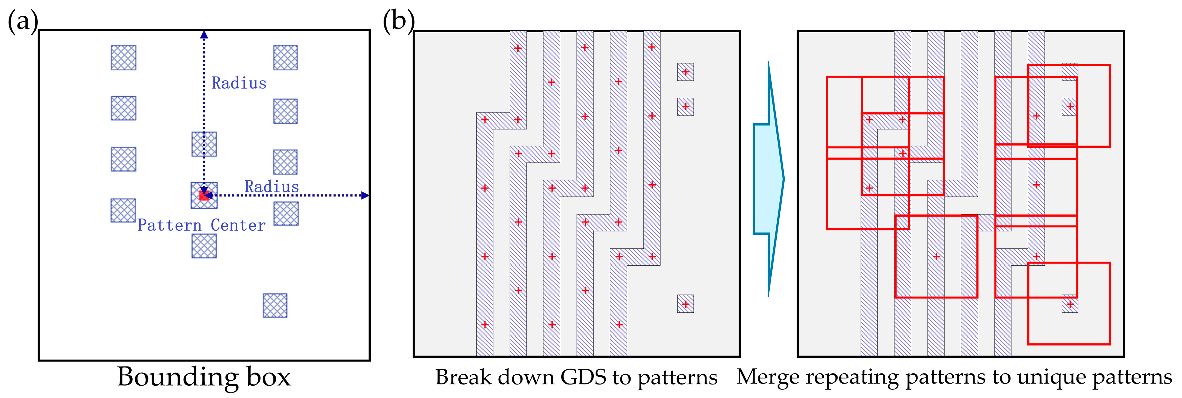
Figure 1. (a) The definition of a pattern. (b) The process of pattern collection.
Photonics 11 00990 g001
Figure 2. Model error distribution of baseline OPC model. The x-axis is a pattern index without solid physical correspondence. Cyan represents 1000 patterns for calibration with 0 outlier patterns. Dark blue is 2425 patterns for verification with 30 outlier patterns.
Photonics 11 00990 g002
Figure 3. OPC model prediction accuracy improved after adding outliers into the calibration. The x-axis is a pattern index without solid physical correspondence. Cyan represents 1030 patterns for calibration with 0 outlier patterns. Dark blue is 2395 patterns for verification with 0 outlier patterns.
Photonics 11 00990 g003
Figure 4. The structure of the AE network.
Photonics 11 00990 g004
Figure 5. The distance ranking result and KL divergence comparison under different FV dimensions: (a) Result for the FV with dimension 49; (b) Result for the FV with dimension 100; (c) Result for the FV with dimension 196; (d) Result for the FV with dimension 400; (e) Result for the FV with dimension 729.
Photonics 11 00990 g005
Figure 6. The PCA visualization of improved AE (a) and basic AE (b) under dimension 49.
Photonics 11 00990 g006
Table 1. The RMS and error range of baseline OPC model.
DatasetRMS (nm)Error Range (nm)
Calibration1.627.94
Verification3.0437.06
Verification excluding outliers2.0915.35
Table 2. The RMS and error range of improved OPC model.
DatasetRMS (nm)Error Range (nm)
Calibration2.0513.56
Verification2.1513.63
Table 3. The loss of AE models with MSE training loss function.
DimensionTraining Loss (×103)Verification Loss (×103)
492.522.61
1001.791.86
1961.301.37
4001.001.07
7290.951.02
Table 4. The loss of AE models with improved training loss function.
DimensionTraining Loss (×104)Verification Loss (×104)
492.542.64
1001.731.81
1961.621.71
4000.610.70
7290.550.66
Disclaimer/Publisher’s Note: The statements, opinions and data contained in all publications are solely those of the individual author(s) and contributor(s) and not of MDPI and/or the editor(s). MDPI and/or the editor(s) disclaim responsibility for any injury to people or property resulting from any ideas, methods, instructions or products referred to in the content.