Complex Noise-Based Phase Retrieval Using Total Variation and Wavelet Transform Regularization

Abstract

This paper presents a phase retrieval algorithm that incorporates sparsity priors into total variation and framelet regularization. The proposed algorithm exploits the sparsity priors in both the gradient domain and the spatial distribution domain to impose desirable characteristics on the reconstructed image. We utilize structured illuminated patterns in holography, consisting of three light fields. The theoretical and numerical analyses demonstrate that when the illumination pattern parameters are non-integers, the three diffracted data sets are sufficient for image restoration. The proposed model is solved using the alternating direction multiplier method. The numerical experiments confirm the theoretical findings of the lighting mode settings, and the algorithm effectively recovers the object from Gaussian and salt–pepper noise.

1. Introduction

Because of the loss of phase information, reconstruct the underlying image from Fourier transform magnitudes is defined as a phase retrieval (PR) problem. Phase retrieval problems are ill-posed, because different images can have the same Fourier transform results, so the solution is not unique. It is necessary to know the image’s prior information, such as domain, nonnegative, sparse representation [1,2], etc., to constrain the numerical process to obtain the global saddle-point solution. Readers can consult [1,2,3] for applications in regularizing seismic image beyond aliasing via gradient and spectral techniques and additional information.

Gerchberg and Saxton [4] proposed an error reduction method (ER) based on projection; later, in 1982, this method was improved by Fienup’s hybrid inputs–outputs (HIO) in [1]. Derived iterative projection algorithms include hybrid projective–reflection [3,5], the iterative difference map (DF) [6] and the relaxed averaged alternation reflection (RAAR) algorithms [7]. In addition, Marchesini adopted the saddle-point optimization method [8] to solve the PR problem. The alternate projection method lacks convergent guarantee because of its alternating projection process that does not have nonconvex constraint sets. Thus, the solution converges to a local stationary point rather than the global optimal solution. Moreover, gradient-type methods have become popular; one example is the Wirtinger Flow (WF) method [9] proposed by Candès, Li and Soltanolkotabi who put forward a gradient scheme with novel update rules that are carefully initialized by the means of a spectral method. Gradient-based approaches usually have first-order convergence. Farrell solved the phase retrieval (PR) problem with a network where every agent only contains a subset of the measurements [10]. A convex method is characterized by the use of convex relationships of the quadratic equations or semidefinite programming. Candès, Strohmer and Voroninski proposed Phaselift in [11], which uses SDP lifting techniques to formulates convex trace (nuclear) norm minimization. Moretta study the impact of constraints in Phaselift in [12]. PhaseCut [13], proposed by Waldspurger, is a convex method that separates phase information and magnitudes. Yin and Xin proposed PhaseLiftOff [14], a nonconvex variant of Phaselift which cut out the Frobenius norm from the trace norm to retrieve phase information with fewer measurements. Xia studied the sparse phase retrieval method to recover a k-sparse signal in [15]. Gao studied the adaptive sparse signal reconstruction algorithm in [16].

In recent years, total variation (TV) regularization has been successfully used to solve image blind deblurring optimization problems with certain specific blurring kernels. In addition, framelet-based regularization has been adopted to solve deblurring problem with motion blur kernels. However, there is huge potential area for them to be used in phase retrieval problems from Fourier transform magnitudes. In this paper, we propose a phase retrieval algorithm based on TV regularization and the analysis-based sparsity framelet transform method to recover the image through an analysis matrix. We explicitly focus on the sparsity of image representation in phase retrieval problems from Fourier transform magnitudes. Total variation regularization can effectively guarantee a sparsity prior for the gradient domain of ground truth images with a small TV semi-norm and framelet transform can enforce a sparsity prior of target images under the redundant tight frame.

In the field of image deblurring and phase recovery, a single Gaussian noise is usually used to test the robustness of phase recovery algorithms against noise. In the field of image denoising, the robustness of the algorithm to salt-and-pepper noise is studied. Gaussian noise and salt-and-pepper noise are typical types of noise, which exist simultaneously in actual measurements. In order to simulate realistic measurement conditions, the reconstruction ability against two kinds of noise is studied for the first time. In order to simulate more realistic measurement conditions, this paper innovatively proposes to study the robustness of the algorithm with complex noise when two kinds of noise exist simultaneously. This is a very challenging problem.

Phase retrieval problems from Fourier transform magnitudes are an ill-posed problem, and these problems are more difficult than phase retrieval problems derived from motion blur. Readers can consult the work [17,18] of E. J. Candes, who studies the relationship between the number of measurements and the possibility of reconstructing an image. For research on further applications for reconstructing images from partial measurements, please see the work of Chang Huibin [19]. On that basis, our research shows that when the illumination source meets a certain parameter setting, three sets of measured values can reconstruct an image.

2. Foundations of Phase Retrieval

2.1. Phase Retrieval Model

Phase retrieval is a branch of deconvolution problems and can be expressed as follows:

$$b=\left|ℱu\right|+\eta$$

(1)

$ℱ : Rea{l}^{n_1\times n_2} \to Comple{x}^{n_1\times n_2}$ is the two-dimensional discrete Fourier transform. $b$ is the measurement magnitude with noise $\eta$. For the convenience of calculation and implementation, we use vectors to represent two-dimensional discrete images in lexicographical order (connected by columns). To more easily present the modules, the symbols do not change. $u$ is defined on a discrete lattice $\mathsf{\Omega }=\left\{0,1,\dots ,n_1\times n_2-1\right\}\to R^{n_1\times n_2}$ of size ${\mathrm{n}}_1\times {\mathrm{n}}_2$, which denotes that image u is connected by columns. The corresponding discrete Fourier transform is expressed as follows:

$$\begin{array}{ll}ℱu({\omega }_1+{\omega }_2{n}_2)=& \frac{1}{\sqrt{n_1{n}_2}}{\displaystyle \sum _{0\le t_1\le n_k-1}{\displaystyle \sum _{\le t_2\le n_k-1}u(t_1+n_1{t}_2)\cdot }}\\ & \exp (-i2\pi (\frac{{\omega }_1{t}_1}{n_1}+\frac{{\omega }_2{t}_2}{n_2})\\ & 0\le {\omega }_1\le n_k-1, 0\le {\omega }_2\le n_k-1\end{array}$$

(2)

2.2. Total Variation

The total variation (TV) model of image processing based on partial differential equation (PDE) variation method is known as the classic Rudin Osher Fatemi (ROF) model in [20]. It is one of the most common models used for image restoration, and generally consists of a fidelity term, regularization penalty items and regularization parameters. In recent years, the TV model is widely used in image denoising and other fields; readers can consult [21,22,23] for detail. Total variation regularization can effectively guarantee a sparsity prior for the gradient domain of the underlying images which have a small norm.

In the following equations, $u$ denotes the image for phase retrieval which is represented as discrete 2-dimensionl matrices with a size of $m\times n$. The total variation in the discrete domain calculates the gradient of u, which is denoted by a gradient operator $\nabla \mathrm{u}$:

$$\begin{array}{l}\nabla {\mathrm{u}}_{p,q}=({\nabla }^1{\mathrm{u}}_{p,q},{\nabla }^2{\mathrm{u}}_{p,q})=(\mathrm{d}x\left({\mathrm{u}}_{p,q}\right),\mathrm{dy}\left({\mathrm{u}}_{p,q}\right))\\ {\nabla }^1{\mathrm{u}}_{p,q}=\{\begin{array}{l}{\mathrm{u}}_{p,q}-{\mathrm{u}}_{p,q+1} if \mathrm{q}<n\\ 0 if \mathrm{q}=\mathrm{n}\end{array}\\ {\nabla }^2{\mathrm{u}}_{p,q}=\{\begin{array}{l}{\mathrm{u}}_{p,q}-{\mathrm{u}}_{p+1,q} if p<m\\ 0 if p=m\end{array}\end{array}$$

(3)

where ${\mathrm{u}}_{p,q}$ is an element of u, ${\nabla }^1{\mathrm{u}}_{p,q}$ is the gradient of the horizontal direction and ${\nabla }^2{\mathrm{u}}_{p,q}$ is the gradient of the vertical direction.

The total variation (TV) regularization term of u is indicated as follows:

$$TV(u)={\displaystyle \sum _{p\le m,q\le n}\left|\nabla {\mathrm{u}}_{p,q}\right|}$$

(4)

For the restoration model with additive noise pollution data, it can be indicated as follows:

$$\begin{array}{l}u=\arg \underset{u}{\min }L(\mathrm{u})\le \epsilon \\ L(\mathrm{u})=\frac{\lambda }{2}{\Vert \left|ℱ\mathrm{u}\right|-b\Vert }_{\mathsf{\Omega }}^2+TV(u)\end{array}$$

(5)

where λ > 0 is the parameter of the total variation regular term. The total variation regularization penalty term is the semi-norm of the image gradient. One type of TV variant, namely the isotropic TV, is defined by

$$\begin{array}{cc}\hfill TV{(u)}_1=& \sqrt{{\left(dx(u)\right)}^2+{\left(dy(u)\right)}^2}\hfill \\ \hfill =& {\displaystyle \sum _{p=1}^{m-1}{\displaystyle \sum _{q=1}^{n-1}\sqrt{{\left(u_{p,q}-u_{p,q+1}\right)}^2+{\left(u_{p,q}-u_{p+1,q}\right)}^2}}}\hfill \\ & +{\displaystyle \sum _{p=1}^{m-1}\left|u_{p,n}-u_{p+1,n}\right|}+{\displaystyle \sum _{q=1}^{n-1}\left|u_{m,n}-u_{q+1}\right|}\hfill \end{array}$$

(6)

Another type is anisotropic TV, which is defined by

$$\begin{array}{cc}\hfill TV{(u)}_2=& dx(u)+dy(u)\hfill \\ \hfill =& {\displaystyle \sum _{p=1}^{m-1}{\displaystyle \sum _{q=1}^{n-1}\left\{\left|u_{p,q}-u_{p,q+1}\right|+\left|u_{p,q}-u_{p+1,q}\right|\right\}}}\hfill \\ & +{\displaystyle \sum _{q=1}^{n-1}\left|u_{m,q}-u_{q+1}\right|}+{\displaystyle \sum _{p=1}^{m-1}\left|u_{p,n}-u_{p+1,n}\right|}\hfill \end{array}$$

(7)

2.3. Wavelet

Images have sparse representation or approximation in redundant transformation, such as tight frame transform [24,25]. Wavelet [26] is one type of tight frame. A large number of studies have shown that sparsity prior and low rank prior regularization enable the corresponding algorithm to produce a high-quality solution [27,28].

2.3.1. Tight Framework

A tight frame in a Hilbert space is introduced as follows, and the interested readers can consult [27] for more in-depth study. Let $\Vert \cdot \Vert$ denote the norm of a variable in a Hilbert space $\mathscr{H}$. The sequence ${\left\{{\varphi }_{\mathrm{n}}\right\}}_{n\in L}\subset \mathscr{H}$ constructs a tight frame in $\mathscr{H}$, when

$$\begin{array}{l}f={\displaystyle \sum _{{\varphi }_n\in }\langle f,{\varphi }_n\rangle }{\varphi }_n , \forall f\in \mathscr{H}\\ {\Vert f\Vert }_2^2={{\displaystyle \sum _{n\in L}\left|\langle f,{\varphi }_n\rangle \right|}}^2, \forall f\in \mathscr{H}\end{array}$$

(8)

where $\langle f,{\varphi }_n\rangle$ indicates an inner product and $\Vert \cdot \Vert$ indicates the norm of $\mathscr{H}$.

For the bounded sequence ${\left\{{\varphi }_{\mathrm{n}}\right\}}_{n\in L}\subset \mathscr{H}$, let $\mathcal{W}$ denote the analysis operator and let ${\mathcal{W}}^{\ast }$ denote its adjoining operator; they are defined by

$$\begin{array}{l}\mathcal{W}: f\in \mathscr{H}\to \left\{\langle f,{\varphi }_n\rangle \right\}\in l^2\left(N\right), \\ {\mathcal{W}}^{\ast }:\left\{a_n\right\}\in l^2\left(N\right)\to {\displaystyle \sum _{n\in L}{a}_n}{\varphi }_n\in \mathscr{H}\end{array}$$

(9)

The sequence ${\left\{{\varphi }_{\mathrm{n}}\right\}}_{n\in L}\subset \mathscr{H}$ constructs a tight frame when ${\mathcal{W}}^{\ast }\mathcal{W}=I$; therein, $I : \mathscr{H}\to \mathscr{H}$ is the identity operator.

In the following equations, u denotes the image for phase retrieval.

$$g=\mathcal{W}\mathrm{u}$$

(10)

$$\mathrm{u}={\mathcal{W}}^{\ast }\left(\mathcal{W}\mathrm{u}\right)={\mathcal{W}}^{\ast }g$$

(11)

where g indicates the tight framelet transform coefficients.

The phase retrieval deconvolution optimization model based on synthetic sparsity representation is

$$\begin{array}{l}\mathcal{W}: \mathrm{u}\in \mathscr{H}\to \left\{\langle u,{\varphi }_n\rangle \right\}\in l^2\left(N\right), \\ {\mathcal{W}}^{\ast }:\left\{a_n\right\}\in l^2\left(N\right)\to {\displaystyle \sum _{n\in L}{a}_n}{\varphi }_n\in \mathscr{H}\end{array}$$

(12)

The deconvolution optimization model based on analytical sparsity representation is

$$\overline{\mathrm{g}}=\underset{u\in R^{m\times \mathrm{n}}}{\arg \min } \mathsf{\Phi }(k\otimes u-f)+\lambda {\Vert g\Vert }_1$$

(13)

The deconvolution optimization model based on synthesis sparsity representation is

$$\begin{array}{l}\overline{g}=R\overline{\mathrm{u}}\\ \overline{\mathrm{u}}=\underset{u\in R^{m\times \mathrm{n}}}{\arg \min } \mathsf{\Phi }(k\otimes u-f)+\lambda {\Vert \mathcal{W}u\Vert }_1\end{array}$$

(14)

The tight frame is one type of orthonormal basis generalization; redundant frame has been found to be useful in image and signal processing [25,29,30]. Analysis operator W is redundant when its column dimension is smaller than the row dimension and the two methods generate different results. The synthesis-based method aims to obtain the most spars result among all possible transform coefficient vectors, while the analysis-based method seeks the most spar solutions among all possible canonical framelet coefficient vectors. Thus, the analysis-based method is a strict subset of synthesized-based methods. The solutions of analysis-based methods are close to the underlying image have increased smoothness. This has been proven empirically in many experiments. Since a solution with a certain smoothness will have a better visual quality, the analysis-based approach was chosen for this study. The two approaches are equivalent only if ${\mathcal{W}}^{\ast }\mathcal{W}=\mathcal{W}{\mathcal{W}}^{\ast }=I$. Then, the tight frame becomes a canonical orthogonal transformation.

2.3.2. Wavelet Tight Framework

A one-dimensional wavelet frame is constructed by a finite set of generators with shifts and dilations, $\mathsf{\Psi }=\left\{{\psi }^1,\dots {\psi }^r\right\}\subset L_2$, where $\psi$ is called the father wavelet and ${\psi }_{j,k}$ is called the wavelet. A refinable function is usually used to construct a tight wavelet frame, $\phi \left(t\right)\in L^2\left(R\right)$, which is also known as the scale function or mother wavelet. This satisfies the two-scale equation ${\widehat{\psi }}^i\left(2\omega \right)=h_i\widehat{\varphi }\left(\omega \right)$, where $h_i$ are $2\pi$ periodic trigonometric polynomials, which satisfies $h_0\left(0\right)=1$.

The unitary extension principle (UEP) [31] declares that $X\left(\mathsf{\Psi }\right)$ forms a tight frame when

$$h_0\left(\omega \right)\overline{h_0\left(\omega +\gamma \pi \right)}+{\displaystyle \sum _{i=1}^r{h}_i\left(\omega \right)\overline{h_i\left(\omega +\gamma \pi \right)}}={\delta }_{\gamma ,0} , \gamma =0,1$$

(15)

Image processing uses two-dimensional information, so the two-dimensional wavelet frames are needed. Indeed, a two-dimensional wavelet is a tensor product of a one-dimensional wavelet. S. Malat and Meyer proposed MRA theory [31,32,33], which studies the multi-resolution analysis properties of wavelets from the perspective of a function space, and provides a unified theory for constructing a wavelet framework and a fast algorithm for orthogonal wavelet transform. In this study, a two-level piecewise linear B-spline tight frame system with tensor product filters was adopted. The piecewise linear B-spline tight frame is the simplest system in this family, which employs piecewise linear B-spline functions as $\phi$. The corresponding tensor product filter is:

$$\begin{array}{ll}{a}_{0,0}=\frac{1}{16} \left(\begin{array}{ccc}1& 2& 1\\ 2& 4& 2\\ 1& 2& 1\end{array}\right)& a_{0,1}=\frac{\sqrt{2}}{16}\left(\begin{array}{ccc}1& 0& -1\\ 2& 0& -2\\ 1& 0& -1\end{array}\right)\\ a_{0,2}=\frac{1}{16}\left(\begin{array}{ccc}-1& 2& -1\\ -2& 4& -2\\ -1& 2& -1\end{array}\right)& a_{1,0}=\frac{\sqrt{2}}{16}\left(\begin{array}{ccc}1& 2& 1\\ 0& 0& 0\\ -1& -2& -1\end{array}\right)\\ a_{1,1}=\frac{1}{8} \left(\begin{array}{ccc}1& 0& -1\\ 0& 0& 0\\ -1& 0& 1\end{array}\right)& a_{1,2}=\frac{\sqrt{2}}{16}\left(\begin{array}{ccc}-1& 2& -1\\ 0& 0& 0\\ 1& -2& 1\end{array}\right)\\ a_{2,0}=\frac{1}{16} \left(\begin{array}{ccc}-1& -2& -1\\ 2& 4& 2\\ -1& -2& -1\end{array}\right)& a_{2,1}=\frac{\sqrt{2}}{16}\left(\begin{array}{ccc}-1& 0& 1\\ 2& 0& -2\\ -1& 0& 1\end{array}\right)\\ a_{2,2}=\frac{1}{16}\left(\begin{array}{ccc}1& -2& 1\\ -2& 4& -2\\ 1& -2& 1\end{array}\right)& \end{array}$$

(16)

MATLAB software R2016b was used for the calculations. We used the wavelet frame decomposition algorithm [25], whose construction varies with boundary setting conditions. In this research, Neumann (symmetric) boundary conditions were adopted. Interested readers can refer to [27,31,34] for the principles of generating such matrices.

3. Proposed Model and Numerical Algorithm

3.1. Formulation of Minimization Model

Our work is closely related to article [17]. where E. J. Candes discussed the possibility of reconstructing the target from incomplete sampling, and ${7\mathrm{n}}_1{\mathrm{n}}_2$ measurements (the size of ground truth image is ${\mathrm{n}}_1\times {\mathrm{n}}_2$) were suggested in order to uniquely recover real-valued images. Chang Huibin proposed a TV regularization [19] model which can recover images from noisy measurements. In this research, a TV and wavelet-based co-exist regularization model is proposed to recover underlying images from ${3\mathrm{n}}_1{\mathrm{n}}_2$ measurements with noise. The measurements were obtained by structured light illumination and image value with box constraint $u_{object}\in \left[0,1\right]$. The model is introduced as follows:

$$\begin{array}{l}find u\\ \mathrm{s}.\mathrm{t}{. \mathrm{b}}_0:=\left|ℱ\left(u_{object}\right)\right|,{ \mathrm{b}}_1:=\left|ℱ\left(u_{object}+D^{\mathrm{s}}{u}_{object}\right)\right|,{ \mathrm{b}}_2:=\left|ℱ\left(\mathrm{u}-\mathrm{i}{D}^{\mathrm{s}}{u}_{object}\right)\right|\end{array}$$

(17)

where $ℱ$ denotes the Fourier transform. Let

$$R\left(u_{object}\right):=\left\{R_0,R_1,R_2\right\}$$

(18)

The data R($u_{object}$) are obtained using three-light-field illumination

$$\left|R(u_{object})\right|=\left\{1, \left|1+\exp (i2\pi (\frac{{\mathrm{s}}_1{t}_1}{n_1}+\frac{s_2{t}_2}{n_2}))\right|, \left|1+\exp (i2\pi (\frac{{\mathrm{s}}_1{t}_1}{n_1}+\frac{s_2{t}_2}{n_2})-\frac{\pi }{2})\right|\right\}$$

(19)

where

$$\begin{array}{l}{D}^{\mathrm{s}}{u}_{object}(t_1+n{t}_2)=\exp (\frac{2\pi s_1+t_1}{n_1}+\frac{2\pi s_2+t_2}{n_2})u_{object}(t_1+t_2{n}_1), \\ 0\le t_1\le n_k-1, 0\le t_2\le n_k-1\end{array}$$

(20)

The research in [19,35] showed that the least square method produces a unique result for the PR problem with these three sets of data. The model is referred to as the least-square minimization problem with a box-constrained (LSB) model [35].

$$\begin{array}{ll}\underset{0\le u\le 1}{\min }& {\Vert \left|R_0\right|-b_0\Vert }_{{\mathsf{\Omega }}_0}^2+{\Vert {\left|R\right|}_1-b_1\Vert }_{{\mathsf{\Omega }}_1}^2\\ & +{\Vert \left|R_2\right|-b_2\Vert }_{\mathsf{\Omega }2}^2\end{array}$$

(21)

This study focused on the sparse prior of objects; we incorporated TV and wavelet transform regularization into (17) to guarantee an exact solution. The analysis-based sparsity approach under wavelet tight frame decomposition was selected for this study. The proposed TV and framelet-based minimization problem of the least-square type with a box constraint (TFLSB) model is presented as follows:

$$\begin{array}{ll}\underset{0\le u\le 1}{\min }{\epsilon }_{TFLSB}=& \frac{\lambda }{2}\left({\Vert \left|R_0\right|-b_1\Vert }_{{\mathsf{\Omega }}_0}^2+{\Vert \left|R_1\right|-b_2\Vert }_{{\mathsf{\Omega }}_1}^2+{\Vert \left|R_2\right|-b_3\Vert }_{\mathsf{\Omega }2}^2\right)\\ & +TV(u)+{\Vert Wu\Vert }_1\end{array}$$

(22)

where we adopt anisotropic TV regularization to be the term of TV(u), $Wu$ is the wavelet decomposition of $u$, and ${\Vert \cdot \Vert }_1$ denotes the L-1 norm.

3.2. Uniqueness Analysis

Hayes [36] and Sanz [37] proved that using double the number of measurements can uniquely determine the solution of PR when the underling signal is nonnegative and finitely supported. The results are further extended with random oversampling [38,39,40], where random illumination guarantees the absolute uniqueness and resolves all types of problems. We found that when $s_1=s_2=N+0.5$ (where N is a positive integer), 3n₁n₂ measurements and additional constraints such as the underlying object $u$ is real and has a non-negative value, the algorithm can produce a unique solution.

Theorem 1.

Assume that $u_{m,n}\in \left[0,1\right]$ and the DFT of u and D^s u are nonvanishing, when s₁ and s₂ are prime with m and n, and s₁ = s₂ = N + 0.5 (N is a positive integer). Then, u can be recovered with 3 mn measurements in (15).

Proof. 

This theorem applies to one-dimensional and two-dimensional cases. The complete proof is shown in Appendix A. □

3.3. Solution Existence Analysis

Theorem 2.

Let Ω denote a bounded set in Lipschitz regular domain and comprehensive data b = (b₀, b₁, b₂) is non-negative; then, the TFLSB model (19) has at least one minimum solution $u$ * ∈ BV (Ω).

Proof. 

It should be noted that ${\epsilon }_{\mathrm{TFLSB} \left(\mathrm{u}\right)} \ge 0$. A minimizing sequence {u_k}_{0 ≤ k ≤ ∞} satisfies (s.t.) ${\epsilon }_{\mathrm{TFLSB} \left(\mathrm{u}0\right)} \ge {\epsilon }_{\mathrm{TFLSB} \left(\mathrm{u}1\right)}\ge \dots$. It is known that $value(u_k)\in \left[0,1\right]$. The set Ω is bounded in a Lipschitz regular domain, C is a positive constant and exists as the upper limit, and s.t. $TV(u_k)+W{u}_k+{\Vert u_k\Vert }_1++{\Vert W{u}_k\Vert }_1\le C$. As Rellich’s compactness theorem state that there is $u^{\ast }\in BV(\mathsf{\Omega })$ and a subsequence ${\left\{u_{nk}\right\}}_{k\ge 1}$, which meet $u_{nk}\to u^{\ast }$ in the norm of $L_1\left(\mathsf{\Omega }\right)$ when $k\to \infty$. Using the continuity of the fidelity term of ${\epsilon }_{TFLSB}$ and lower semi-continuity of TV and wavelet regularization, one obtains $\underset{u_{nk}\to u\ast }{\lim \sup }{\epsilon }_{TFLSB}(u_k){\ge }_{TFLSB}(u\ast )$. Then, u* is the one solution of ${\epsilon }_{TFLSB}$. □

3.4. Numerical Model

There are several numerical methods that are used for the constrained optimization problem. At present, the Projected Gradient Descent (PGD) and Alternating Direction Method of Multipliers (ADMM) are widely used. The Alternating Direction Method of Multipliers (ADMM) was first proposed by Glowinski and Gabay, and further improved by Boyd in 2011, who demonstrated that ADMM is applicable in large-scale distributed optimization problems [41]. ADMM is a computational method for optimization problems, and is effective in solving distributed convex optimization problems, especially statistical learning problems [42,43]. Through the process of decomposition–coordination, ADMM disassembles the large complicated global problem into several smaller solvable local sub-problems, which can be computed more easily and could converge to the global optimal solution through the coordination of the sub-problems. The disadvantages of the Projected Gradient Descent method are as follows: (1) it may converge to the local optimal solution; (2) the differential at saddle point is 0, but it is not the optimal solution; (3) because of its computational complexity, it is a time-consuming method, especially when the data is large-scale. Thus, ADMM was selected to solve the constrained optimization problem in this paper.

The above minimum problem model can be described by the formula:

$$\begin{array}{ll}\min & {\Vert {\mathrm{p}}_1\Vert }_1+{\Vert {\mathrm{p}}_2\Vert }_1+\frac{\lambda }{2}{\Vert \left|z_0\right|-b_0\Vert }_{{\mathsf{\Omega }}_0}^2+\frac{\lambda }{2}{\Vert \left|z_1\right|-b_1\Vert }_{\mathsf{\Omega }1}^2\\ & +\frac{\lambda }{2}{\Vert \left|z_2\right|-b_2\Vert }_{{\mathsf{\Omega }}_2}^2+\chi \left(v\right)\\ s.t.& v=u p_1=\nabla u p_2=wu z_0=R_0 z_1=R_1 z_2=R_2\end{array}$$

(23)

where

$$\chi \left(\mu \right)=\{\begin{array}{l}0, 0\le \mathrm{v}\le 1\\ \infty , \mathrm{otherwise}\end{array}$$

(24)

The augmented Lagrangian equation of ${ℒ}_{TFLSB}$ reads

$$\begin{array}{cc}ℒ(u,z_0,z_1,z_2,p,v)& ={\Vert {\mathrm{p}}_1\Vert }_1+{\Vert {\mathrm{p}}_2\Vert }_1+\frac{\lambda }{2}{\Vert \left|z_0\right|-b_0\Vert }_{{\mathsf{\Omega }}_0}^2\hfill \\ & +\frac{\lambda }{2}{\Vert \left|z_1\right|-b_1\Vert }_{\mathsf{\Omega }1}^2+\frac{\lambda }{2}{\Vert \left|z_2\right|-b_2\Vert }_{{\mathsf{\Omega }}_2}^2+\chi \left(v\right)\hfill \\ & +R\langle d_0,z_0-R_0\rangle +\frac{{\rho }_1}{2}{\Vert z_0-R_0\Vert }_{{\mathsf{\Omega }}_0}^2\hfill \\ & +R\langle d_1,z_1-R_1\rangle +\frac{{\rho }_1}{2}{\Vert z_1-R_1\Vert }_{\mathsf{\Omega }1}^2\hfill \\ & +R\langle d_2,z_2-R_2\rangle +\frac{{\rho }_1}{2}{\Vert z_2-R_2\Vert }_{{\mathsf{\Omega }}_2}^2\hfill \\ & +\langle q_1,p_1-\nabla u \rangle +\frac{{\rho }_3}{2}{\Vert p_1-\nabla u\Vert }_2^2\hfill \\ & +\langle q_2,p_2-Wu \rangle +\frac{{\rho }_4}{2}{\Vert p_2-Wu\Vert }_2^2\hfill \\ & +\langle w,u-v\rangle +\frac{{\rho }_2}{2}{\Vert u-v\Vert }_2^2+t{\Vert Hv\Vert }^2\hfill \\ & ={\Vert {\mathrm{p}}_1\Vert }_1+{\Vert {\mathrm{p}}_2\Vert }_1+\frac{\lambda }{2}{\Vert \left|z_0\right|-b_0\Vert }_{{\mathsf{\Omega }}_0}^2\hfill \\ & +\frac{\lambda }{2}{\Vert \left|z_1\right|-b_1\Vert }_{\mathsf{\Omega }1}^2+\frac{\lambda }{2}{\Vert \left|z_2\right|-b_2\Vert }_{{\mathsf{\Omega }}_2}^2+\chi \left(v\right)\hfill \\ & +\frac{{\rho }_1}{2}{\Vert z_0-R_0+\frac{d_1}{{\rho }_1}\Vert }_{{\mathsf{\Omega }}_0}^2+\frac{{\rho }_1}{2}{\Vert z_1-R_1+\frac{d_2}{{\rho }_1}\Vert }_{{\mathsf{\Omega }}_1}^2\hfill \\ & +\frac{{\rho }_1}{2}{\Vert z_2-R_2+\frac{d_3}{{\rho }_1}\Vert }_{{\mathsf{\Omega }}_2}^2+\frac{{\rho }_2}{2}{\Vert u-v+\frac{w}{{\rho }_2}\Vert }_2^2\hfill \\ & +\frac{{\rho }_3}{2}{\Vert p_1-\nabla u+\frac{q_1}{{\rho }_3}\Vert }_2^2+\frac{{\rho }_4}{2}{\Vert p_2-Wu+\frac{q_2}{{\rho }_4}\Vert }_2^2\hfill \\ & +t{\Vert Hv\Vert }^2\hfill \end{array}$$

(25)

where $q_1,q_1:\mathsf{\Omega }\to R^2$, $Hv$ is the position penalty term of the image, and $\lambda ,{\rho }_1,{\rho }_2,{\rho }_3,{\rho }_4$ are weight parameters and are positive. The ADMM solution framework for the above saddle-point solution, minimizes ${ℒ}_{TFLSB}$ with regardto $u,z,p,\mathrm{v}$ alternately and then update the dual variables $d_0$, $d_1$, $d_2$, $d_3$ and $q_1,q_2$. The algorithm is summarized in the Algorithm 1.

According to the ADMM algorithm, the solution is decomposed into the following steps.

Algorithm 1 ADMM method for solving the TFLSB model (22)

Initialization:

$\begin{array}{l}k=0, z_i^0=b_i\left(\omega \right)\exp (-2\pi i{\theta }_i),\\ {\mathrm{p}}^0=0,{ \mathrm{v}}^0=0,{ \mathrm{d}}_i^0=0, q_1{}^0=0, q_2{}^0=0\end{array}$

While the loop stop conditions are not satisfied, do

$u^{k+1}=\underset{u}{\arg \min }{L}_{TFLSB}\left(u,z_i{}^k,p_1{}^k,p_2{}^k,v^k,d_i{}^k,w^k,q_1{}^k,q_2{}^k\right)$

$z_i{}^{k+1}=\underset{z_i}{\arg \min }{L}_{TFLSB}\left(u^k,z_i,p_1{}^k,p_2{}^k,v^k,d_i{}^k,w^k,q_1{}^k,q_2{}^k\right)$

$p_1{}^{k+1}=\underset{p_1}{\arg \min }{L}_{TFLSB}\left(u^k,z_i{}^k,p_1,p_2{}^k,v^k,d_i{}^k,w^k,q_1{}^k,q_2{}^k\right)$

$p_2{}^{k+1}=\underset{p_2}{\arg \min }{L}_{TFLSB}\left(u^k,z_i{}^k,p_1{}^k,p_2,v^k,d_i{}^k,w^k,q_1{}^k,q_2{}^k\right)$

$v^{k+1}=\underset{v}{\arg \min }{L}_{TFLSB}\left(u^k,z_i{}^k,p_1{}^k,p_2{}^k,v,d_i{}^k,w^k,q_1{}^k,q_2{}^k\right)$

Update dual variables

$\{\begin{array}{l}{d}_1{}^{k+1}=d_1{}^k+{\rho }_1\left(z_0{}^{k+1}-R_0{}^{k+1}\right)\\ d_2{}^{k+1}=d_2{}^k+{\rho }_1\left(z_1{}^{k+1}-R_1{}^{k+1}\right)\\ d_3{}^{k+1}=d_3{}^k+{\rho }_1\left(z_2{}^{k+1}-R_2{}^{k+1}\right)\\ w^{k+1}=w^k+{\rho }_2\left(u^{k+1}-v^{k+1}\right)\\ q_1{}^{k+1}=q_1{}^k+{\rho }_3\left(p^{k+1}-\nabla u^{k+1}\right)\\ q_2{}^{k+1}=q_2{}^k+{\rho }_4\left(p_2{}^{k+1}-w{u}^{k+1}\right)\end{array}$

k = k + 1

end while

output the solution $u^{\ast }=u^{k+1}$

The subproblem to solve the saddle point of u is

$$\begin{array}{ll}\underset{u}{\min }& \frac{{\rho }_3}{2}{\Vert p-\nabla u+\frac{q_1}{{\rho }_3}\Vert }^2+\frac{{\rho }_4}{2}{\Vert p_2-Wu+\frac{q_2}{{\rho }_4}\Vert }_2^2+\frac{{\rho }_2}{2}{\Vert u-v+\frac{q_2}{{\rho }_2}\Vert }^2\\ & +\frac{{\rho }_1}{2}{\Vert z_0-ℱu+\frac{d_1}{{\rho }_1}\Vert }_{{\mathsf{\Omega }}_0}^2+\frac{{\rho }_1}{2}{\Vert z_1-ℱ\left(\mathrm{u}+D^{\mathrm{s}}u\right)+\frac{d_2}{{\rho }_1}\Vert }_{{\mathsf{\Omega }}_1}^2\\ & +\frac{{\rho }_1}{2}{\Vert z_2-ℱ\left(\mathrm{u}-\mathrm{i}{D}^{\mathrm{s}}u\right)+\frac{d_3}{{\rho }_1}\Vert }_{{\mathsf{\Omega }}_2}^2\end{array}$$

(26)

By calculating the derivative, the solution is

$$\begin{array}{c}-\Delta u+\frac{{\rho }_2}{{\rho }_3}u+\frac{{\rho }_4}{{\rho }_3}u+\frac{{\rho }_1}{{\rho }_3}\left(5I+2R\left(D^{\mathrm{s}}\right)+2E\left(D^{\mathrm{s}}\right)\right)u\\ =\frac{{\rho }_1}{{\rho }_3}\left(\begin{array}{l}R\left({ℱ}^{\ast }\left(z_0+\frac{d_1}{{\rho }_1}\right)\right)\\ +R\left({ℱ}^{\ast }\left(z_1+\frac{d_2}{{\rho }_1}\right)+D^{\mathrm{s}}\overline{{ℱ}^{\ast }\left(z_1+\frac{d_2}{{\rho }_1}\right)}\right)\\ +R\left({ℱ}^{\ast }\left(z_2+\frac{d_3}{{\rho }_1}\right)-i{D}^{\mathrm{s}}\overline{{ℱ}^{\ast }\left(z_2+\frac{d_3}{{\rho }_1}\right)}\right)\end{array}\right)\\ +\frac{{\rho }_2}{{\rho }_3}\left(v-\frac{q_2}{{\rho }_2}\right)-div\left(p_1+\frac{q_1}{{\rho }_3}\right)+\frac{{\rho }_4}{{\rho }_3}{W}^T\left(p_2+\frac{q_2}{{\rho }_4}\right)\end{array}$$

(27)

4. Numerical Experiments

The initialization method for the proposed Algorithm 1 is as follows.

The measurements b_i containing noise are used directly for the calculations without any processing. The initial phase is given randomly without any specific request.

The initialization for variables $v_0$ and $z_i^0$ was chosen to be

$$z_i^0\left(\omega \right)=\{\begin{array}{cc}{b}_i\left(\omega \right)\exp (-2\pi i{\theta }_0)\hfill & \hfill \mathrm{if}\omega \in \mathsf{\Omega }\\ 0\hfill & \hfill \mathrm{otherwise}\end{array}$$

(28)

and $v^0=ℱz_0^0=ℱ\left(b_0\left(\omega \right)\exp (-2\pi i{\theta }_0) \right)$, where initial phase ${\theta }_0$ is derived from the standard uniform distribution in the open interval (0, 1).

The quality of the reconstructed image includes two aspects: one is the visual effect and the other is the evaluation index to analyze the difference between the reconstructed image and original image. The evaluation of visual effects varies with different people’s visual conditions. Objective evaluation indicators are very important. The affluent evaluation index of the reconstruction image evaluation used in the field of image reconstruction was adopted in this study to compare the proposed algorithm with other algorithms.

The peak signal-to-noise ratio (PSNR), structural similarity (SSIM) and signal-to-noise ratio (SNR) were used to measure the quality of the reconstruction, and the relative error (relative-error) was used to measure the convergence speed. PSNR is a comprehensive evaluation index of reconstruct image quality. MSE is the mean square error of the current calculated image compared to the ground truth image. H and V represent the number of the row and column, respectively, and n is the number of bits of storage per pixel.

$$\begin{array}{l}MSE=\frac{1}{H\ast v}{\displaystyle \sum _{p=1}^H{\displaystyle \sum _{q=1}^v{\left(u\left(p,q\right)-u_g\left(p,q\right)\right)}^2}}\\ PSNR=10{\log }_{10}\left(\frac{{\left(2^{\mathrm{H}\times \mathrm{V}}-1\right)}^2}{MSE}\right)\end{array}$$

(29)

SSIM (structural similarity) is a comprehensive evaluation of the image restoration quality in terms of brightness, contrast and image structure.

$$\begin{array}{l}{\mu }_u=\frac{1}{H\ast V}{\displaystyle \sum _{i=1}^H{\displaystyle \sum _{j=1}^{V}u\left(p,q\right)}}\\ {\sigma }_u=\frac{1}{H\ast V-1}{\left({{\displaystyle \sum _{i=1}^H{\displaystyle \sum _{j=1}^V\left(u\left(p,q\right)-{\mu }_u\right)}}}^2\right)}^{\frac{1}{2}}\\ {\sigma }_{u_g}=\frac{1}{H\ast W-1}{\displaystyle \sum _{i=1}^H{\displaystyle \sum _{j=1}^W\left(u\left(p,q\right)-{\mu }_u\right)}}\left(u_g\left(p,q\right)-{\mu }_u\right)\\ l\left(u,u_g\right)=\frac{2{\mu }_u{\mu }_{u_g}+C_1}{{\mu }_u{}^2{\mu }_{u_g}{}^2+C_1}\\ c\left(u,u_g\right)=\frac{2{\sigma }_u{\sigma }_{u_g}+C_2}{{\sigma }_u{}^2{\sigma }_{u_g}{}^2+C_2}\\ s\left(u,u_g\right)=\frac{{\sigma }_{u,u_g}+C_3}{{\sigma }_u{\sigma }_{u_g}+C_3}\\ SSIM=l\left(u,u_g\right)\ast c\left(u,u_g\right)\ast s\left(u,u_g\right)\end{array}$$

(30)

In general, let $C_1=6.5 C_2=58.5 C_3=29$.

Signal-to-noise ratio (SNR) is calculated as

$$\begin{array}{l}RMSE\left(u,u_g\right)=\frac{{\displaystyle \sum _{j\in \mathsf{\Omega }}{\left|u\left(p,q\right)-u_g\left(p,q\right)\right|}^2}}{{\displaystyle \sum _{j\in \mathsf{\Omega }}{\left|u\left(p,q\right)\right|}^2}}\\ SNR\left(u,u_g\right)=-10{\log }_{10}RMSE\left(u,u_g\right)\end{array}$$

(31)

Relative-error is defined as follows:

$$relative-error=\frac{\Vert u\left(p,q\right)-u_g\left(p,q\right)\Vert }{u_g\left(p,q\right)}$$

(32)

In all the above formulas, u represents the current reconstructed image and $u_g$ represents the ground truth image.

4.1. Numerical Results

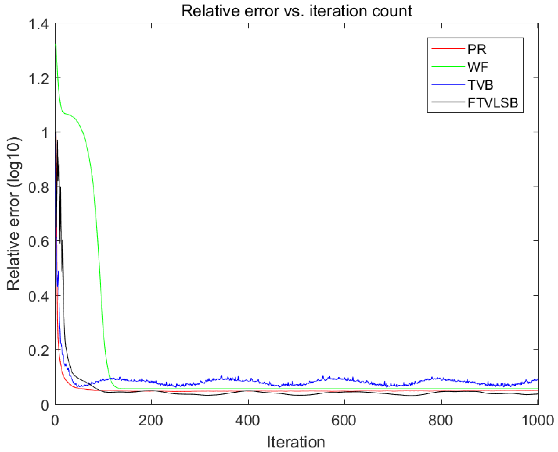
We also compared the PR results for the performance of the proposed TFLSB model with three other related phase retrieval algorithms: the error reduction algorithm (ER) [3], TVB method [18] and Wirtinger flow (WTF) method [9]. The data were contaminated by the Gaussian noise $b_i=b_0+\sigma n_i$, where $b_0$ is magnitudes of the original image, $\sigma$ represents the noisy weight, $n_i$ represents the white Gaussian noise, and $b_i$ is the measurement of the real object’s Fourier transform magnitude.

The test simulation images are available on the Internet (no copyright restrictions). Our research focused on the phase retrieval problem from Fourier transform magnitudes. Its application field covers remote target imaging. Therefore, the selected images have obvious geometric features and simple textures, with a size of 256 × 256.

In order to study the algorithm’s robustness to noise, 60 dB Gaussian noise was added to the measured value to verify the robustness of the algorithms. The noise level was set according to the SNR formula and rand function.

$$\begin{array}{cc}\hfill SNR& =-10{\log }_{10}\frac{{\displaystyle \sum _{j\in \mathsf{\Omega }}{\left|u\left(i,j\right)-u_g\left(i,j\right)\right|}^2}}{{\displaystyle \sum _{j\in \mathsf{\Omega }}{\left|u\left(i,j\right)\right|}^2}}\hfill \\ & =-10{\log }_{10}\frac{{\displaystyle \sum _{j\in \mathsf{\Omega }}{\left|\left|noise\left(i,j\right)\right|\right|}^2}}{{\displaystyle \sum _{j\in \mathsf{\Omega }}{\left|u\left(i,j\right)\right|}^2}}\hfill \end{array}$$

(33)

The TVB method and the TFLSB algorithm use the same structured illumination pattern in this study; the relevant parameters were set as follows: the iteration numbers were 1000, $\lambda =100$, ${\rho }_1=0.07$, ${\rho }_2=0.02$ and ${\rho }_3=0.08$. As $s_1=s_2=N+0.5$ (N is a positive integer) proves that the underlying image has an optimal solution, then s₁ and s₂ can be set to 0.5, 1.5 and 2.5. Here, in this experiment, we set $s_1=s_2=0.5$. Other value settings, such as 1.5, 2.5 and 3.5, could also obtain visually good reconstructed images and can be modified according to different graphics. The results are shown in the following figures, Figure 1, Figure 2, Figure 3, Figure 4, Figure 5 and Figure 6.

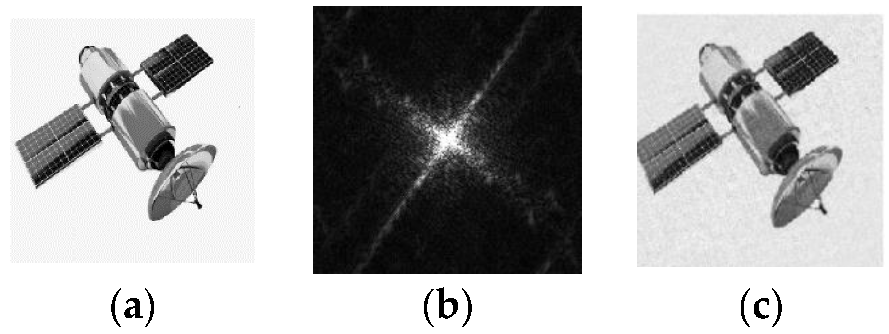
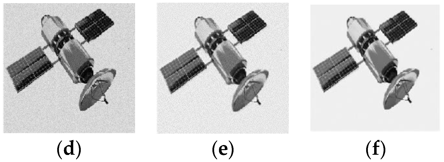
The numerical evaluation index performance of the phase retrieval method reflects the approximate degree of the distribution characteristics of the calculated image and the real object. Image vision includes sharpness, smoothness and similarity. The comparison results of the reconstructed image quality from the three images in Figure 1, Figure 3 and Figure 5 were as follows. Firstly, the ER and TVB algorithms introduced obvious defects in the originally smooth background area. Secondly, the reconstructed image of the ER algorithm was fuzzy overall, while the reconstructed image of WF was sharper. This is because these algorithms do not have a good balance between image smoothness and boundary sharpness. Although the constrained performance of the TVB algorithm was better, its staircase effect can produce obvious defects which could not be omitted. Overall, compared with the other algorithms, the proposed TFLSB model using the ADMM algorithm performed better, and the reconstructed images were more visually pleasant with few noticeable image artifacts.

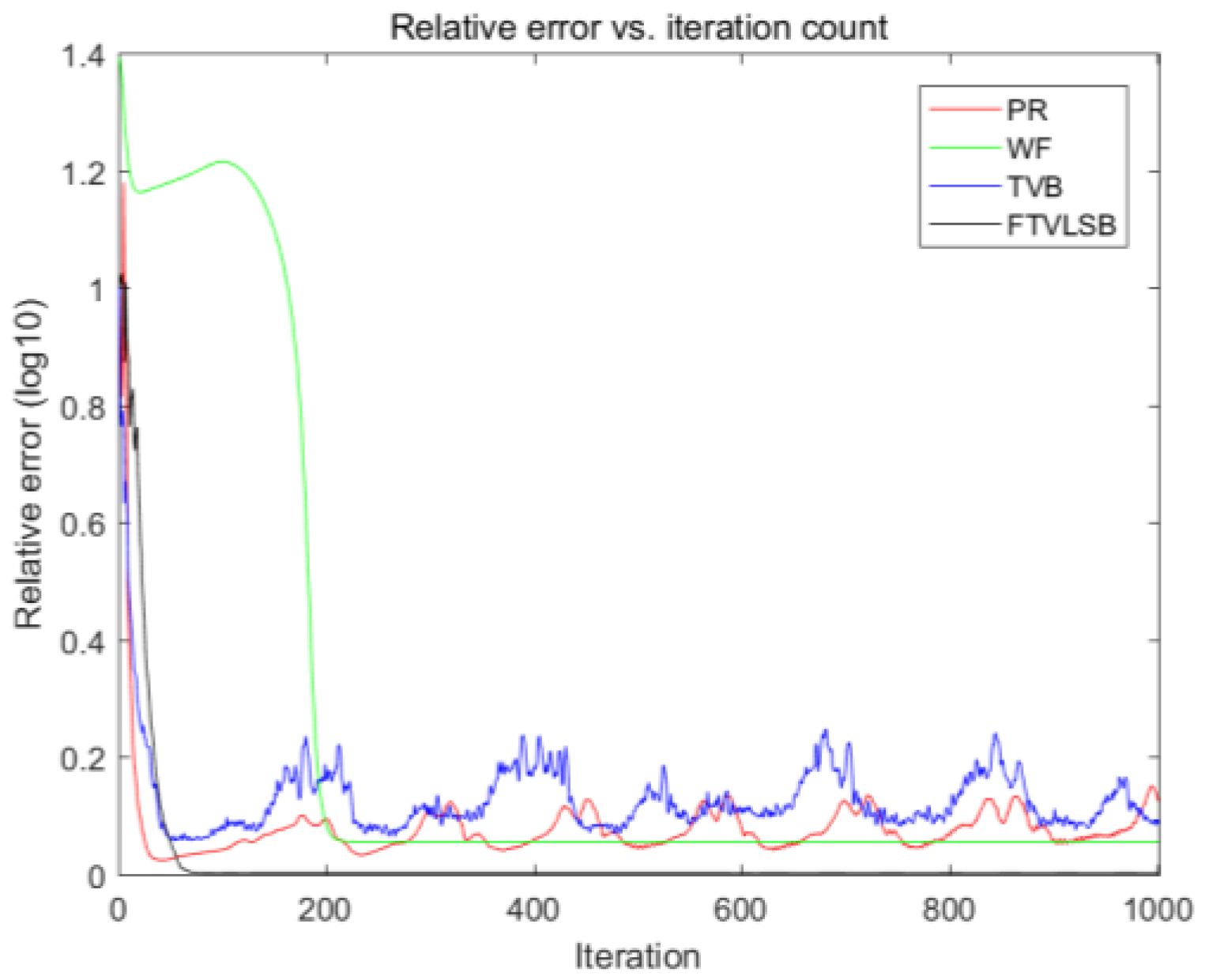
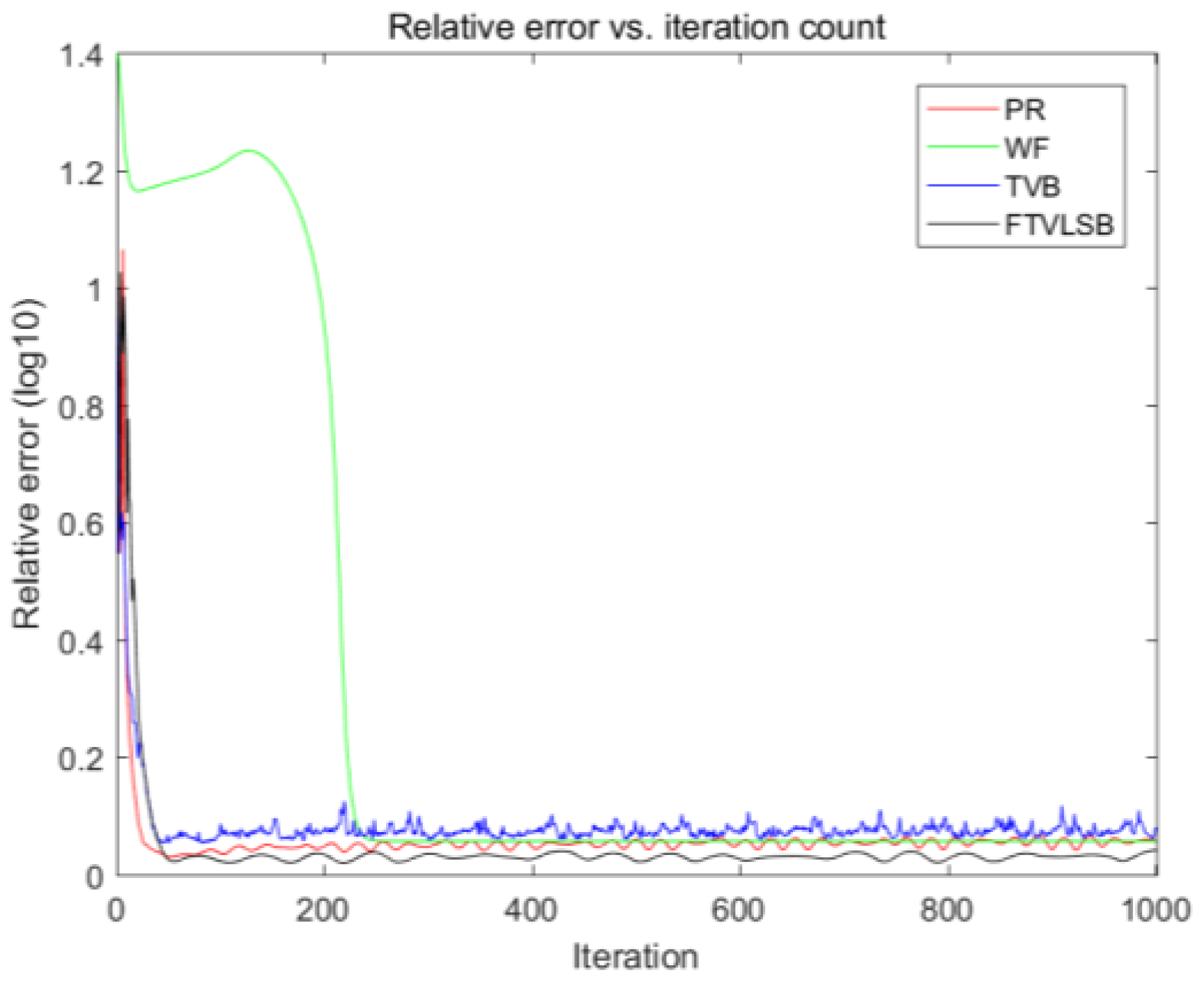
The comparison results in Figure 2, Figure 4 and Figure 6 show that the proposed algorithm was more stable, converged to the optimal value and always had the lowest relative error value when dealing with images with different complexities.

Table 1. Phase retrieval image quality evaluation parameters for different reconstruction algorithms for pine-tree image. The best data are shown in bold.

Method	Time (s)	PSNR	SSIM	SNR (dB)
ER	15.4121	13.8215	0.062745	3.31793
WF	23.8868	17.5721	0.1232	9.45358
TVB	18.1098	23.3189	0.121072	15.7823
TFLSB	36.5556	44.8056	0.166499	47.5823

,

Table 2. Phase retrieval image quality evaluation parameters for different reconstruction algorithms for six-claw image. The best data are shown in bold.

Method	Time (s)	PSNR	SSIM	SNR (dB)
ER	15.783	19.3888	0.120204	9.33326
WF	35.14	16.2947	0.154068	6.28477
TVB	25.1905	23.4579	0.184836	14.2892
TFLSB	46.7172	36.6348	0.535543	45.7626

and

Table 3. Phase retrieval image quality evaluation parameters for different reconstruction algorithm for satellite image. The best data are shown in bold.

Method	Time (s)	PSNR	SSIM	SNR (dB)
ER	12.0018	23.0435	0.271731	10.5373
WF	24.9471	19.0969	0.301472	6.78469
TVB	18.7448	22.7706	0.243096	10.4753
TFLSB	39.7584	28.264	0.305235	32.5247

show the image restoration quality with the numerical evaluation indicators, PSNR, SSIM, SNR and processing time. When the iteration number was 1000, our algorithm required more time due to the algorithm’s computing complexity. However, according to the speed of iterative convergence, the solving time could be shortened by reducing the iteration number. The PSNR, SSIM and SNR indexes directly reflect the pixel correspondence between the reconstructed image and the original image. According to the results of the three reconstructed images, for the TFLSB model proposed in this paper, compared with ER, WF and TVB algorithm, the PSNR index was improved by 111.59%, 108.87% and 57.14%, respectively. The SSIM index improved by 174.49%, 194,74% and 84.37%, and the SNR index improved by 674.89%, 517.72% and 241.47%, respectively. The comparison results in Table 1, Table 2 and Table 3 directly show that our proposed FLSB model is more robust to noise and more efficient in reconstructing images compared to the other methods.

4.2. Sensitivity with Complex Noise

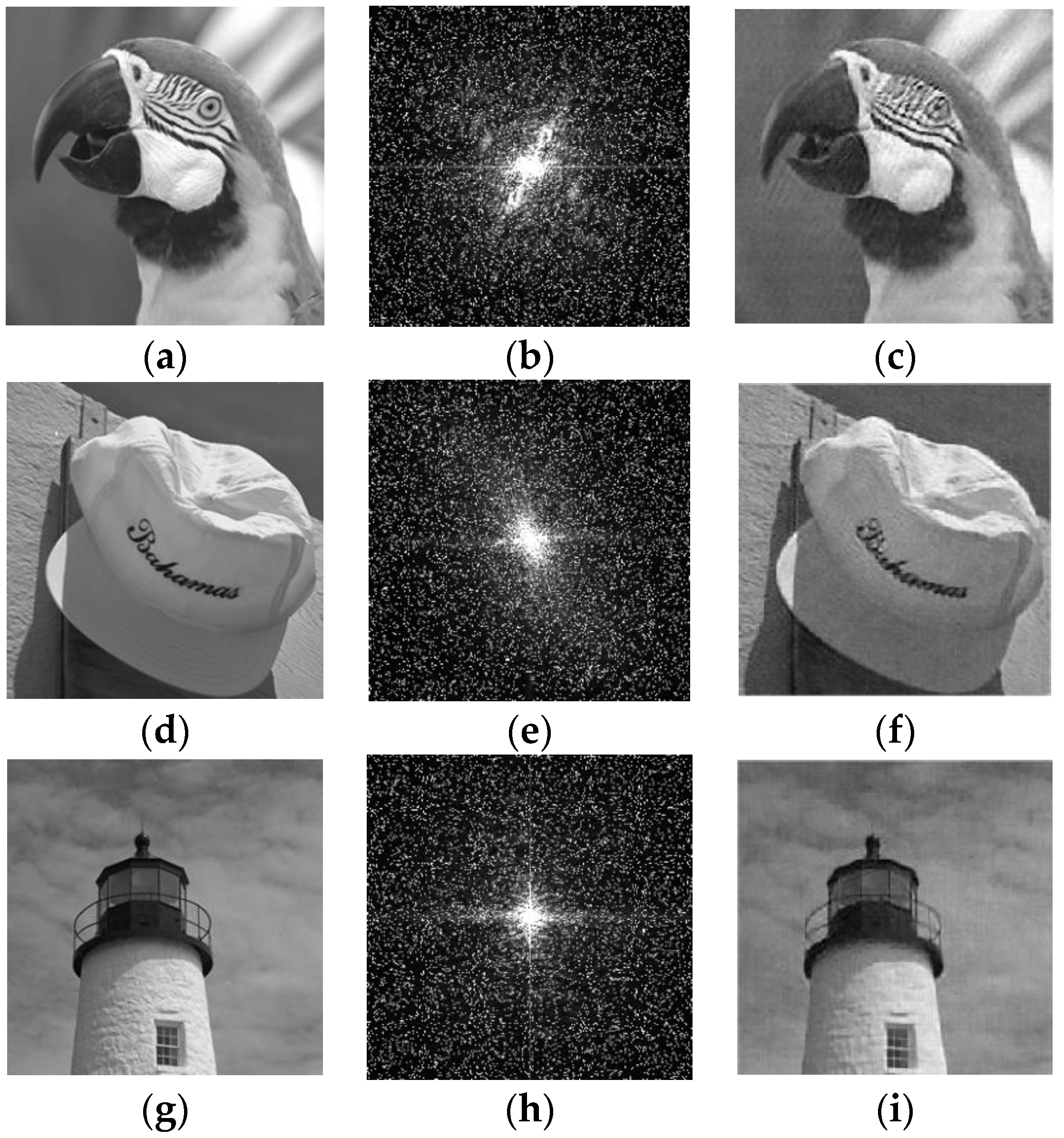
Image acquisition not only contains Gaussian noise, but also electromagnetic interference in the environment, and sensor internal errors, which will introduce salt–pepper noise. Salt–pepper noise, also known as pulse noise, is represented in the image as discrete distributions of pure white or black pixels. The image reconstruction ability of the TFLSB model was studied in images where Gaussian noise and salt–pepper noise coexist. Due to the excellent performance of the proposed algorithm in the previous task, in this experiment, we challenged the proposed algorithm to deal images with more complex textures to study its robustness in the presence of complex noise. The images are public images released by the Kodak Company. For the sake of consistency in this paper, the images used below are part of the original Kodak images, with a size of 256 × 256. Images were named—“Bird”, “Hat”, “Tower”.

The data were contaminated with Gaussian noise and salt–pepper noise, i.e., $b_i=b_0+\sigma n_i+p$, where $b_0$ is the magnitudes of the spatial spectrum of the original image, $\sigma$ represents the noisy weight, $n_i$ represents the white Gaussian noise, p denotes the salt–pepper noise, and $b_i$ is the measurement of the Fourier transform magnitude of the real object. The salt–pepper noise was generated by a random function and threshold setting. First, a random matrix was generated, whose values were derived from the standard uniform distribution in the open interval (0, 1). Then, using the threshold setting, the elements of a random matrix were converted to integers 0 or 1.

Thus, the complex noise is described using the following formula:

$$n_{complex}=\sigma n_i+p$$

(34)

In this experiment, $\sigma$ = 1 and the threshold setting of salt–pepper noise is 0.9. When the value generated by the random function is greater than 0.9, white noise is obtained. The salt–pepper noise setting means that 10% of the measurements were corrupted, which is more serious than a real experiment. The results are shown in the following Figure 7.

By comparing the reconstructed images with the original images, we can observe that the reconstructed images with complex noise have significant clarity regarding visual quality. The numerical values in

Table 4. Parameters of reconstruction result with complex noise.

Name	Time (s)	PSNR	SSIM	SNR (dB)
Bird	35.632	23.605	0.420935	24.7175
Hat	36.2162	26.3138	0.355219	25.1869
Tower	38.1924	29.4759	0.443401	27.188

show that the PSNR values of the restored images varied from 23.606 to 29.4759, the SSIM values varied from 0.355219 to 0.443401, and the SNR values varied from 24.715 dB to 27,188 dB. These data suggest that the proposed sparse prior regularization model TFLSB is robust even with complex noise, and it is also effective in processing images with complex textures. In the future, its application range could be determined by studying the relationship between noise standards, parameter settings and image complexity.

5. Experimental Results

Experimental equipment was set up to simulate reconstruction of the underlying image using Fourier transform magnitudes. The process consisted of two parts. The first part was data collection, during which the spatial spectrum modulus of the target underwent correlation computing. The second is to use the phase recovery algorithm to calculate the reconstructed image.

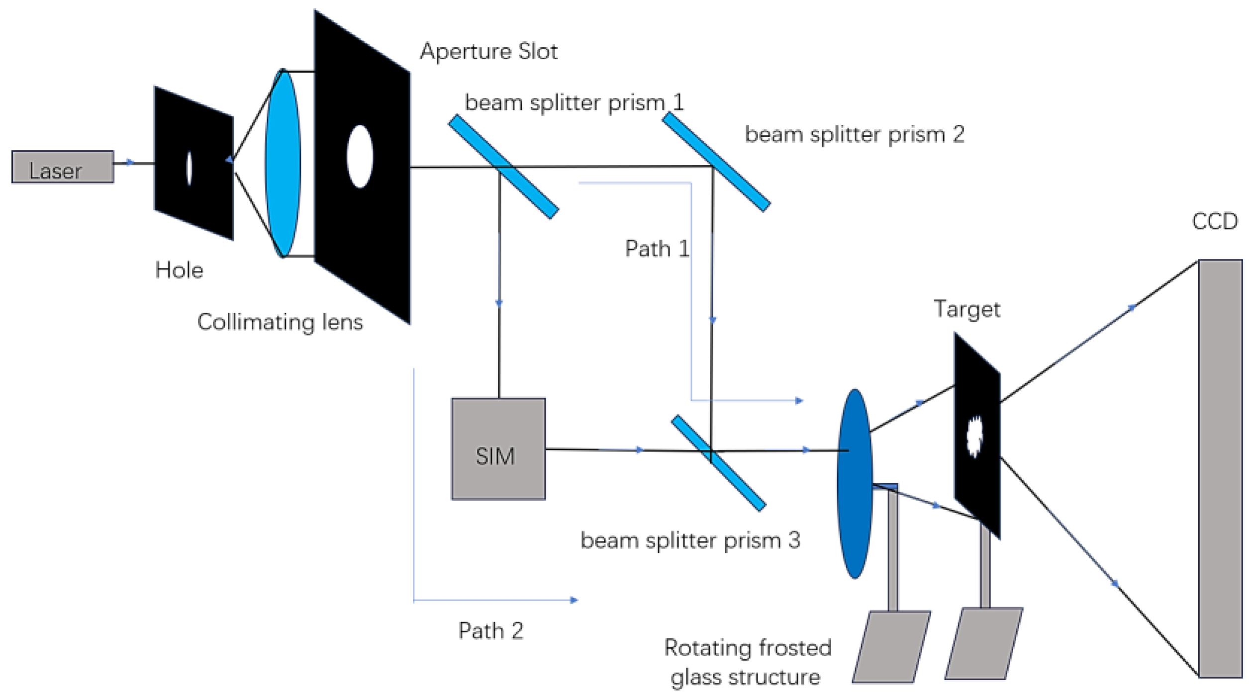
The schematic diagram of the experiment is shown in Figure 8. The working wavelength selected for the laser for the purpose of the experiment was 532 nm. The laser turned into a pseudothermal light source after passing through the rotating glass. In order to reduce the extra stray light caused by reflection, this experiment adopted a transmission target, which was made by hollowing out a target pattern on a metal plate, with an image size of 3 × 3 mm. The structure is shown in Figure 9.

The pixel size of the CCD camera was 6.5 μm, and the number of detection units is 2048 × 2048. In the experiment, the CCD detection frequency was 20 Hz, and the exposure time was 30 ms. The glass rotation speed was 0.3°/s. A SIM structured light modulator was set up using the internal DMD array to realize the control of the structured light. The light field distribution of structured light mode 1 is $\exp (i2\pi (\frac{{\mathrm{s}}_1{t}_1}{n_1}+\frac{s_2{t}_2}{n_2})$. When ${\mathrm{s}}_1={\mathrm{s}}_2=0.5$, it is a two-dimensional sinusoidal distribution of phases in box constrained interval (0-Π). The light field distribution of structured light mode 1 is $\exp (i2\pi (\frac{{\mathrm{s}}_1{t}_1}{n_1}+\frac{s_2{t}_2}{n_2})-\frac{\pi }{2})$, and compared to pattern 1, it has a phase shift.

In order to reduce the influence of the environment on the phase retrieval experiment, data acquisition was divided into two steps. First, when the measurement was not illuminated by a light source, the measurement values $I_{dark}$ of the experimental environment used for imaging and the inherent defects of the measurement system recorded with the detector, representing the background noise. Then, when the light source illuminates the target, the measurement values $I_1,I_2,I_3$ were recorded. The difference between these two points can offset the impact of some of the noise.

The TFLSB algorithm in this paper is used for phase retrieval, and the results are shown in Figure 10.

Due to the limited experimental conditions, the acquisition frequency of the CCD camera was limited, as was the target spatial spectrum information that could be obtained by the pseudothermal light source, making the obtained target information very scarce and increasing the difficulty of phase recovery. When structured light lit an area, the two optical paths should be at the same frequency and there should be no phase delay, but in practical applications, it is difficult to ensure that the optical path difference between the two optical paths is 0. This error reduces reconstructed image quality. From the visual evaluation, the resolution of the reconstruction image is not good enough when compared the previous numerical simulation. The evaluation indexes PSNR, SSIM and SNR used for image restoration are not ideal, and additional research on phase retrieval should be carried out in the future. The numerical results in

Table 5. Parameters of reconstruction result.

Name	PSNR	SSIM	SNR (dB)
Object1	8.71775	0.00939781	12.2024
Object2	7.2705	0.00304378	11.3587

directly show that our proposed FLSB model could efficiently reconstruct images in practice.

6. Conclusions

In this paper, we introduced an innovative TV and framelet-based regularization minimization phase retrieval model with a box constraint (TFLSB) for image recovery from magnitudes degraded by Gaussian and salt–pepper noise. Our proposed model incorporates isotropic TV and analysis-based wavelet regularization, enabling the enforcement of sparse priors in both the gradient domain and spatial structure domain simultaneously. Through heuristic analysis, we identified the key parameters s₁ = s₂ = N + 0.5 (N being a positive integer) that contribute to stable phase recovery with 3n₁n₂ measurements. This structural light can be easily obtained by using a structured light modulator. The TFLSB model effectively reconstructs high-quality latent images from corrupted measurement data obtained with a structured lighting model. Comparative evaluations against the ER, WF, and TVB algorithms demonstrate that the degraded images reconstructed by the TFLSB model exhibit superior image quality, with clearer edges and fewer artifacts. The evaluation indices PSNR, SSIM and SNR further confirm the significant enhancement in image quality achieved by the numerical theory and TFLSB model. Additionally, our study investigated the robustness of the TFLSB model against Gaussian and salt–pepper noise, revealing its resilience against complex noise. This provides a certain direction for the implementation of phase retrieval from Fourier transform magnitudes in practice.

Furthermore, in practice, the proposed method is able to reconstruct the underlying image from Fourier transform magnitudes, helping us to solve the phase retrieval problem in environments. Under the existing experimental conditions, the reconstructed images solved using the TFLSB algorithm are not clear enough, but there is an optimal solution, that can verify the stability and feasibility of the proposed algorithm.

It is important to note that phase retrieval remains a challenging deconvolution problem, and there are several open questions that require further exploration. The proposed algorithm was the most time consuming compared to the other algorithms, which is not conducive to real-time imaging applications. One potential improvement is the use of a more powerful industrial computer to reduce the computation time. Future work will focus on developing faster algorithms with a second-order convergence rate to reduce processing time. Additionally, we aim to incorporate more priors to enhance the quality of the reconstructed solutions for a broader range of image categories. While the proposed phase retrieval model is currently applicable to oversampling scenarios (structured illuminated patterns), our future research will explore additional patterns to enable the exact recovery of latent images in various settings.