High-Linear Frequency-Swept Lasers with Data-Driven Control

Abstract

The frequency-swept laser (FSL) is applied widely in various sensing systems in the scientific and industrial fields, especially in the light detection and ranging (Lidar) area. However, the inherent nonlinearity limits its performance in application systems, especially in the broadband frequency-swept condition. In this work, from the perspective of data-driven control, we adopt the reinforcement learning-based broadband frequency-swept linearization method (RL-FSL) to optimize the control policy and generate the modulation signals. The nonlinearity measurement system and the system simulator are established. Since the powerful learning ability of the reinforcement learning algorithm, the linearization policy is optimized off-line and the generated modulation signals reduce the nonlinearity almost 20 times, compared to the case without control. In the long-term operation, the regular updated modulation signals perform better than the traditional iteration results, demonstrating the efficiency of the proposed data-driven control method in application systems. Therefore, the RL-FSL method has the potential to be the candidate of optical system control.

1. Introduction

The frequency-swept laser (FSL) plays a significant role in various scientific and industrial applications ranging from the lasing remote system [1], medical imaging [2], and the optical communication system [3] to precision detection [4,5]. Therefore, the characteristics of the FSL have received widespread attention in research. Taking the application of the FSL in precision detection as an example, the swept bandwidth of the FSL is proportional to the space resolution as it serves as the light source. Therefore, in order to achieve the high-fidelity detection, the broadband swept frequency is highly anticipated. However, the inherent nonlinearity of the FSL is exacerbated in this case. In applications, this distorted relationship leads to errors when inverting the measurement results. Therefore, how to achieve broadband linear frequency sweep is one of the research hotspots.

Currently, the research on the frequency-swept linearization can be roughly divided into two main approaches: the active control [6,7,8] and the passive control [9,10,11,12,13]. The active control approach is represented by the closed-loop correction approach. For example, the phase-locked-loop-based (PLL-based) methods [8] locked the optical frequency sweep to an external reference signal with an auxiliary branch, producing a negative feedback loop. However, the precision of the PLL-based methods relies on high-precision optical components. Moreover, the intense nonlinearity makes it difficult for the loop to achieve a stable clocked state, which limits its adaptability to the broadband frequency-swept linearization.

The passive control approach also requires the auxiliary branch to obtain the reference signal. For example, the resample method [9] utilized the reference signal as the external clock to resample the detection signal at equal optical frequency intervals. Therefore, the nonlinearity in the data acquisition time interval is compensated, which is sensitive to the mismatch between the signals. Moreover, according to the Nyquist–Shannon sampling theorem, the maximum detection range is limited by the delayed length of the auxiliary interferometer. To overcome these limitations, the Hilbert transform is used to compensate the nonlinearity, requiring a phase unwrapping procedure to extract the nonlinear components of the beat frequency generated from the auxiliary interferometer.

Another passive correction approach focuses on producing a pre-distorted modulation current waveform using different iterative methods [10,12]. These approaches are capable of generating high linear frequency-swept light and are independent of specific lasers. But, the optimal parameters for the pre-distortion technique still depend on lasers, requiring a substantial amount of trial-and-error to guarantee the convergence efficiency and the linearization effect.

Both of these passive methods rely heavily on plenty of real-time data collected from the auxiliary branch, while the implicit system characteristics in the data have not been fully explored. The auxiliary branch increases the application system complexity as well. Therefore, a data-driven method is necessary and has the potential to reduce system complexity and improve experimental data efficiency.

In this work, we propose the reinforcement learning (RL) method to linearize the broadband frequency sweep with the data-driven control method. RL is a branch of machine learning. It provides a state-of-the-art solution for the control task, formalized as the Markov decision process (MDP) [14] in various science and industry fields, such as autonomous driving [15], energy management [16], and traffic control [17]. Initially, the agent has no a priori knowledge of the internal functioning or dynamics of the environment. The control policy is optimized during the process that the agent observes states of the environment, produces actions, and receives rewards. According to whether the state transition function and the reward function are known or not, the RL method is separated into model-free RL and model-based RL. Model-free RL is a trial-and-error learner relying on the direct interaction with the environment. It is efficient in capturing environmental characteristics. But, the practicality is limited by the high sample complexity. On the contrary, the model-based RL is considered as a promising planning approach to decrease the sample complexity. The introduction of the probabilistic model extracts the uncertainty characteristics and leads to the model-based RL matching model-free asymptotic performance in challenging domains while using fewer samples. Moreover, the introduction of deep learning makes the deep RL powerful and widely applicable in the complex control tasks. In optics, the integration of the RL develops rapidly as in fields of adaptive optics [18], quantum optics [19], and optical communication networks [20].

In terms of the reinforcement learning-based broadband frequency-swept linearization (RL-FSL), the linearization task is converted to the MDP problem by defining the proper state, action, and reward. Considering efficiency, sample complexity, and safety, we prefer a model-based approach for the broadband frequency-swept linearization task. We establish the FSL nonlinearity measurement system with the FSL and the Mach–Zehnder interferometer (MZI) as the key components, and simulate the system with the experimental data and the random factors as the environment of RL. Based on the twin delayed deep deterministic policy gradient (TD3) algorithm, the characteristics of the FSL are learned and the linearization policy is optimized. The well-trained policy is employed to the experimental frequency measurement system to demonstrate the linearization efficiency of the RL-FSL. Therefore, the proposed method accomplishes the off-line optimization of the linearization policy by fully leveraging the valuable information from experimental data and simplifies the application system of the FSL.

2. Methodology

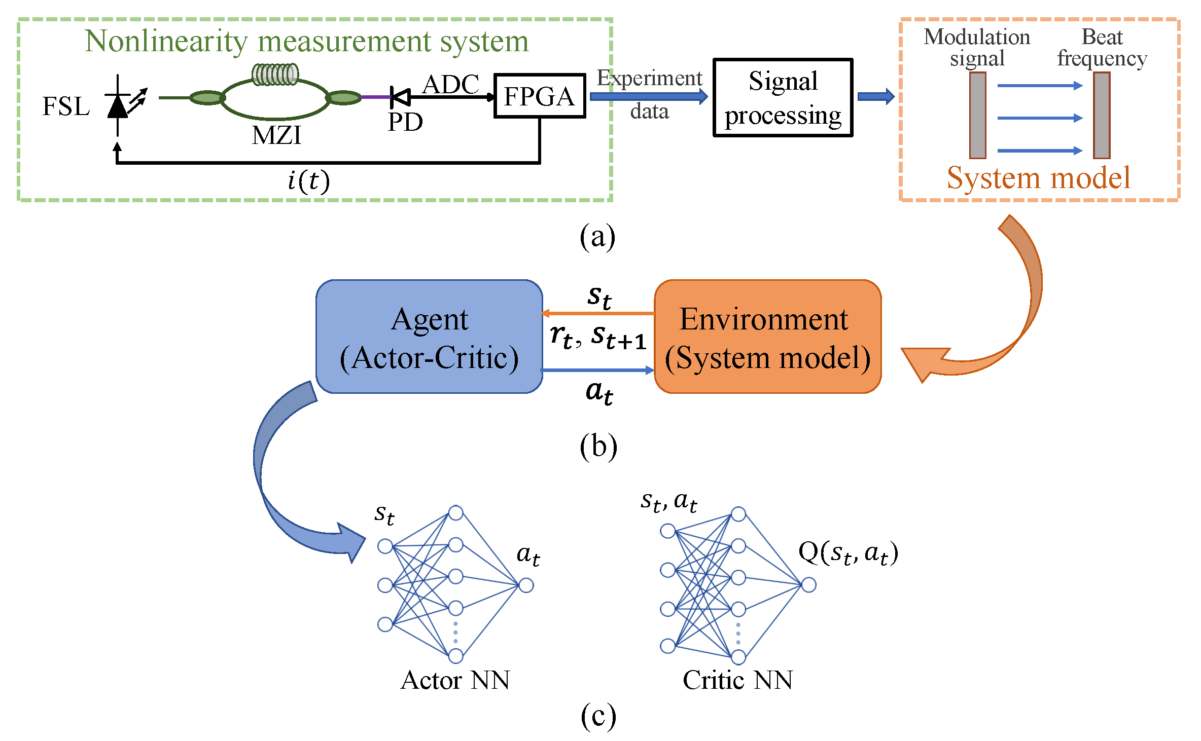
The schematic of the RL is shown in Figure 1b. At each discrete temporal step t, the agent receives the state $s_t$ to perceive environmental characteristics, and delivers the action $a_t$ to modify the environment evolution based on the current control policy. After the environment performs the action, the reward $r_t$ is given to the agent representing the evaluation of the quality of the state–action pair. The received reward and the next step state $s_{t+1}$ are collected to optimize the control policy. The objective of the agent is to optimize the control policy to maximize the cumulative reward. Before converting the broadband frequency-swept linearization task to the MDP, we design the nonlinearity measurement system and establish the system simulator as the RL environment, as shown in Figure 1a.

Assume the chirp frequency of the FSL is represented as:

$$f\left(t\right)=f_0+ki\left(t\right)+f_{nl}\left(t\right)=f_0+F\left(i\left(t\right)\right),$$

(1)

where $f_0$ is the initial frequency, $i\left(t\right)$ is the modulation current, $f_{nl}\left(t\right)$ is the nonlinearity term, and $F\left(·\right)$ represents the mapping relationship of the modulation current and the chirp frequency. Based on the optical interference principle, the frequency of the beat signal collected by the photodetector (PD) is represented as:

$$f_b\left(t\right)=\frac{df\left(t\right)}{dt}=\xi +f_{nl}^{\prime }\left(t\right)=F^{\prime }\left(i\right)·i^{\prime }\left(t\right),$$

(2)

where $\xi =k\frac{di\left(t\right)}{dt}$ and $F^{\prime }\left(i\right)$ is capable to describe the transfer characteristic of the nonlinearity measurement system. According to Equation (2), the beat frequency reflects the nonlinear situation. If the beat frequency is constant, the frequency sweep is linear. Conversely, the nonlinearity exists.

Considering that the high sample complexity [21] of the agent interacts with the experimental system directly during the control policy optimization process, we utilize the experimental data to simulate the system characteristic. According to Equation (2), we collect the input and output data of the system and calculate the corresponding numerical form of $F^{\prime }\left(i\right)$. Simultaneously, we invite the noise term $n\left(t\right)$ [22] to simulate the impact of the random factors in the system. Therefore, we obtain the system simulator, i.e., the RL environment.

$$f_{b,m}\left(t\right)=G\left(i\right)·i^{\prime }\left(t\right)+n\left(t\right),$$

(3)

where $G\left(i\right)$ is the numerical form of $F^{\prime }\left(i\right)$. To accomplish the broadband frequency-swept linearization, a proper modulation current is required. Therefore, the modulation slope of each time step t in the modulation period is controlled and defined as the action $a_t$. Additionally, the state and the reward are defined on the modulation current and the beat frequency.

$$s_t=norm\left([i\left(t\right),f_{b,m}\left(t\right),f_{b,m}\left(t\right)-f_{b,m}(t-1)]\right),$$

(4)

$$r_t=-norm\left(\right|f_{b,m}\left(t\right)-f_{b,r}\left|\right),$$

(5)

where $norm\left(x_i\right)=(x_i-x_{i,min})/(x_{i,max}-x_{i,min})$, and $f_{b,r}$ is the reference frequency. Consequently, we implement the conversion of the broadband frequency-swept linearization problem to the MDP. According to the principle of the RL as shown in Figure 1b, the agent perceives the nonlinear characteristics of the environment with the received state $s_t$, and the modulation slope $a_t$ is delivered to the environment based on the current linearization policy. After performing the modulation current, the next beat frequency is calculated and the linearization efficiency is evaluated by the reward $r_t$. The control policy would be optimized during this process.

Since the action space and the state space are continuous, from a perspective of deep RL, the actor-critic-based algorithms are well-suited. Commonly, the actor-critic structure contains a pair of neural networks (NNs) with different optimization objectives, as shown in Figure 1c. The actor neural network (NN) optimizes the control policy, outputting the action according to the input state. And, the critic NN fits the state-action value function to estimate the current policy of the actor NN. 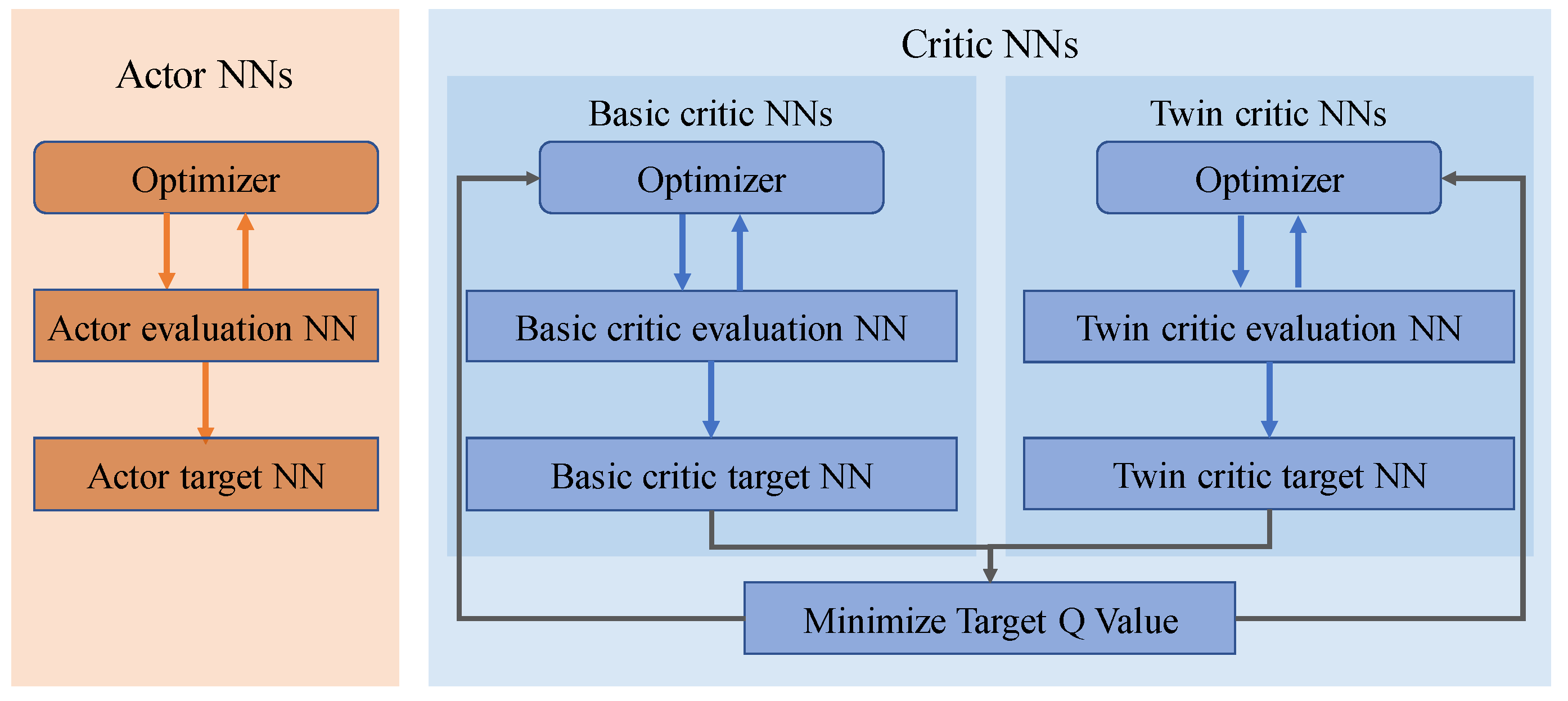We employ the TD3 [23] algorithm to solve the broadband frequency-swept linearization problem, which is one of the state-of-the-art and actor-critic-based algorithms. The TD3-based agent is shown as in Figure 2. The actor NNs of the TD3 contain the actor evaluation NN and the actor target NN. They are parameterized as $\mu \left(s\right|{\theta }^{\mu })$ and ${\mu }^{\prime }\left(s\right|{\theta }^{{\mu }^{\prime }})$, separately. And, the critic NNs of the TD3 contain the basic critic evaluation NN, the basic critic target NN, and their twin NNs. They are parameterized as $Q_i(s,a|{\theta }^{Q_i})$ and $Q_i^{\prime }(s,a|{\theta }^{Q_i^{\prime }})$, separately. The parameter $i=1, 2$ represents the label of basic critic NNs and twin critic NNs. The actor evaluation NN is designed as four fully connected layers $[3,128,256,1]$. The rectified linear unit (ReLU) is used as the activation function of the input and hidden layers. And, the hyperbolic tangent function is connected with the output layer. For the structures of the critic evaluation NNs, they also have four fully connected layers $[4,128,256,1]$. And, the activation functions of these layers are ReLU.

The loss function of the actor evaluation NN is defined as:

$${\nabla }_{{\theta }^{\mu }}J=\mathbb{E}\left[{\nabla }_{{\theta }^{\mu }}{Q}_1(s,a|{\theta }^{Q_1})\right|s=s_t,a=\mu \left(s_t\right|{\theta }^{\mu })],$$

(6)

where ${\theta }^{\mu }$ is the hyper-parameter of the evaluation actor NN. And, the learning rate of the actor NNs is set to 0.001. The basic critic evaluation NN and the twin critic evaluation NN have different initial parameters and are trained separately. The loss functions of networks are defined as:

$$L\left({\theta }^{Q_i}\right)=\mathbb{E}\left[{(Q_i(s_t,a_t|{\theta }^{Q_i})-y_t)}^2\right],$$

(7)

$$y_t=r(s_t,a_t)+\gamma mi{n}_{i=1,2}\left[Q_i^{\prime }(s_{t+1},{\mu }^{\prime }\left(s_{t+1}\right|{\theta }^{{\mu }^{\prime }})+ϵ|{\theta }^{Q_i^{\prime }})\right],$$

(8)

where ${\theta }^{Q_i}$ ($i=1, 2$) are the hyper-parameters of the evaluation critic NNs, and $ϵ\sim \mathcal{N}(0,\delta )$. And, the learning rate of the critic NNs is set to 0.0001. The target NNs have the same structure with the evaluation NNs, and the parameters are update based on:

$${\theta }^{\prime }\leftarrow k\theta +(1-k){\theta }^{\prime }$$

(9)

where $\theta$ and ${\theta }^{\prime }$ represent the parameters of the evaluation NNs and the target NNs, separately, and $k=0.01$ represents the update rate. The update frequency of the actor target NN is half of the critic target NNs.

In the early training process, the actor evaluation NN generates the modulation current according to the initial state and random policy, and the reward and the next state are calculated by the simulator. The collected experiences are stored in the replay-buffer. Until the capacity of the buffer reaches the batch size, the training data are sampled from the buffer. The maximum capacity of the buffer is set to 1,300,000, and the batch size is set to 4096. The whole training process includes 1500 periods and, in each period, the agent interacts with the simulator 3278 times, corresponding to the controlled time steps of the modulation current in the modulation period. And, the data in the replay-buffer is updated continuously. To ensure the exploration–exploitation trade-off of the agent, the executed action of the simulator contains the output of the actor NN and the exploration noise. The variance of the noise gradually decreases with the training process. Consequently, with the convergence of the NNs, the optimized control policy is obtained, and the modulation current is generated during the interactions of the agent and the simulator. Since the random term in the simulator, the generated modulation current is slightly changed in each period. With the regular updated modulation current, it would be more flexible to the random changes in the application system.

3. Results and Discussion

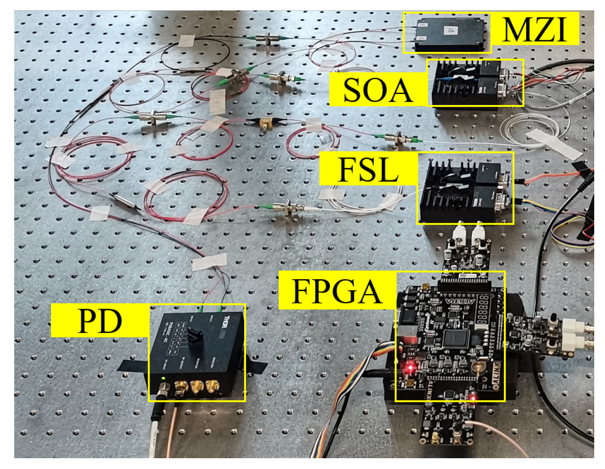
As a proof-of-concept, the nonlinearity measurement system is established to demonstrate the feasibility of the RL-FSL as shown in Figure 3. It starts with a 1550 nm distributed feedback laser (DFB) operating at 25 °C. The DFB FSL provides a frequency modulated continuous wave (FMCW) signal with 1 ms periodic duration driven by an initial sawtooth modulation current. The bandwidth of the frequency sweep is 120 GHz. The emitted optical signal passes through the isolator and enters the semiconductor optical amplifier (SOA). The current-frequency tuning of the laser is accompanied by a parasitic amplitude modulation from the perspective of constructing a swept frequency laser. The amplitude modulation can be corrected with a second feedback loop varying the injection current of the SOA. The equalized light is fed into the MZI with a delay time $\tau =5$ ns and the generated beat signal is collected by the PD. Transferred to the computer by the field programmable gate array (FPGA), the frequency of the beat signal is extracted using the Hilbert transition. According to the collected beat frequency and the modulation slope, the nonlinear mapping relationship is calculated. Along with the random term, the system simulator is built and employed as the RL environment. The following policy optimization process is finished on the computer. The generated modulation current is transferred by the FPGA and updated regularly to guarantee the stable linearization efficiency.

To evaluate the performance of the data-driven control, we compare it with the classical methods, and calculate the root mean square of the residual nonlinearity (RMSRN) as the metric according to the bandwidth of the beat signal [13].

$$\delta f_b=2(1+2\pi \tau f_{nl,rms})f_m,$$

(10)

where $f_m$ is the modulation frequency. In addition, to further analyze the impact of the nonlinearity to the actual application, we make the frequency modulated continuous wave light detection and ranging (FMCW LiDAR) as an example and calculate the theoretical space resolution (TSR).

$$\delta d=\frac{c}{2\delta f·f_m}\delta f_b,$$

(11)

where c is the speed of light, and $\delta f$ represents the bandwidth of the frequency sweep.

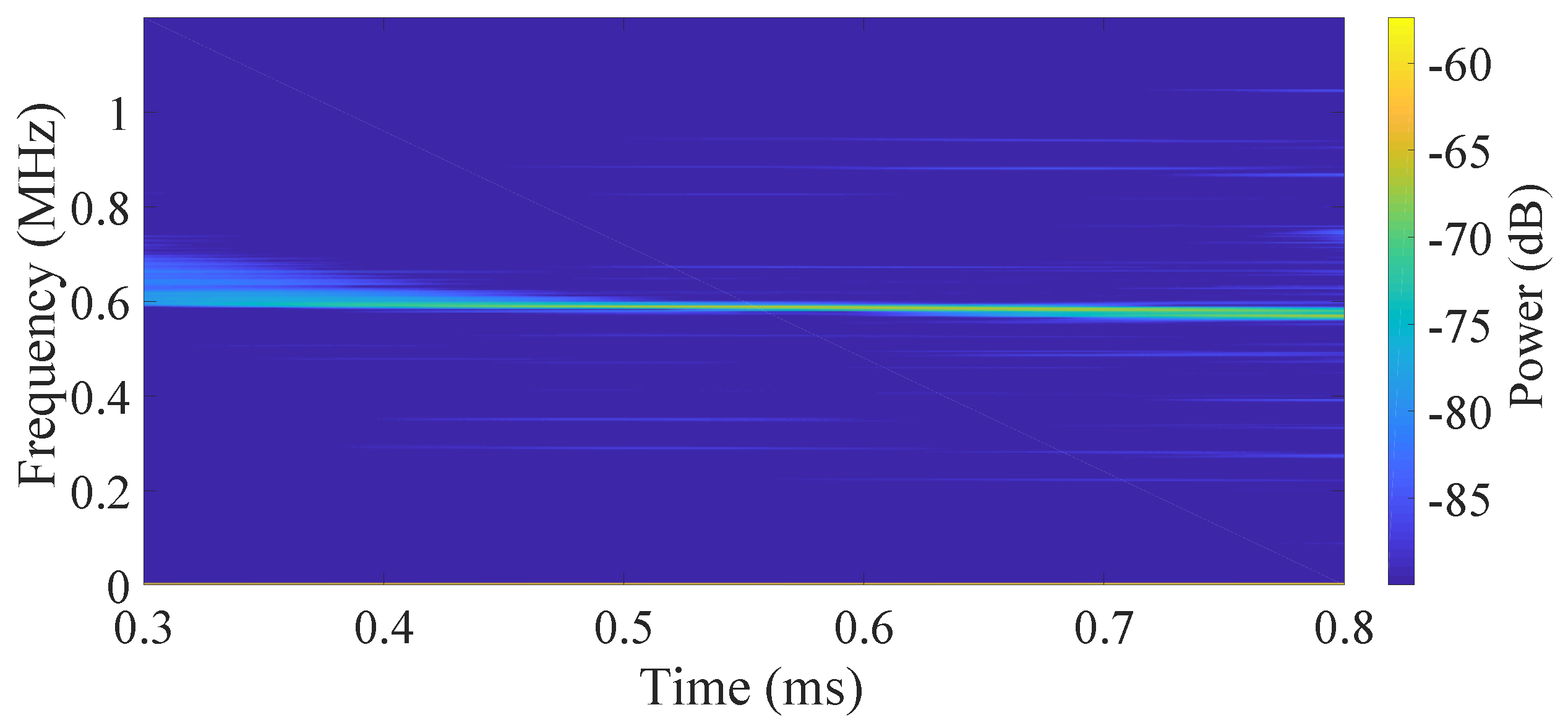
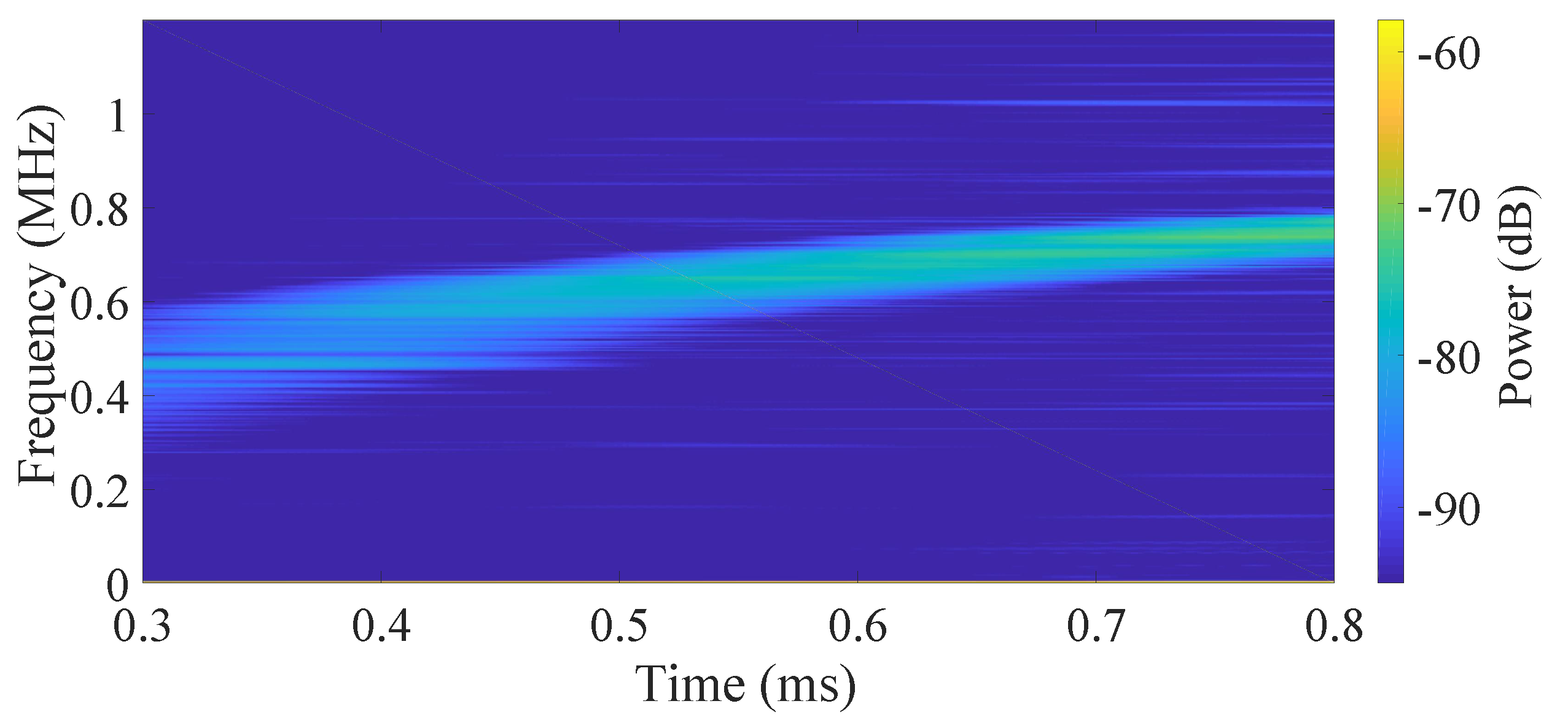
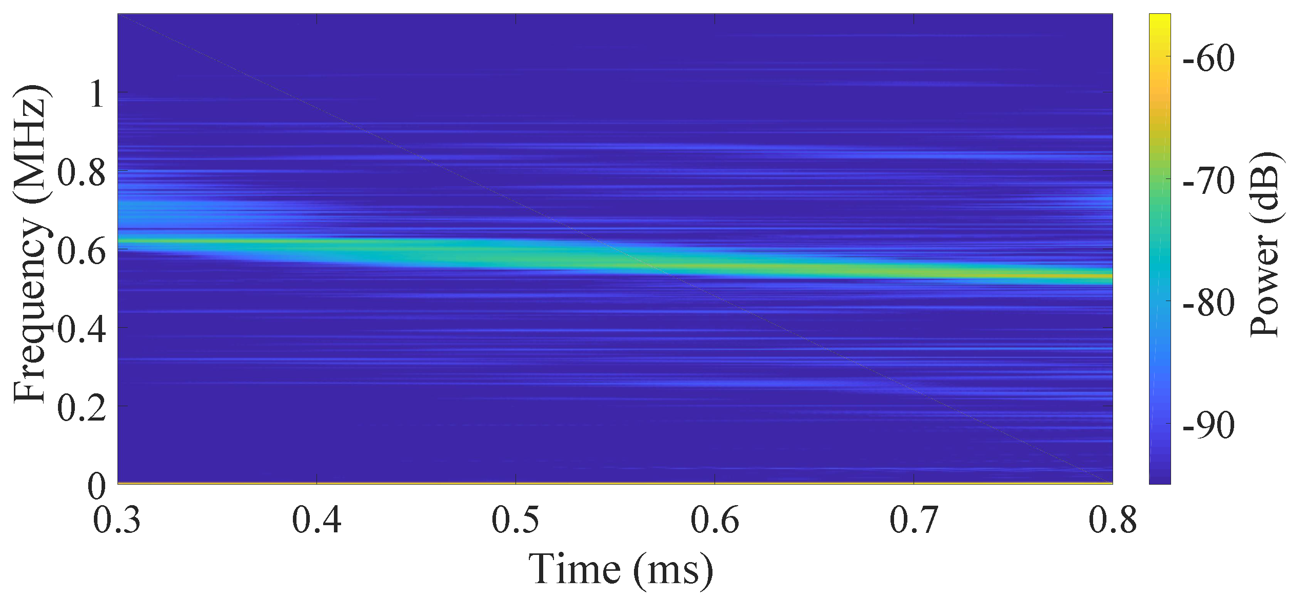
The spectrum analysis of the beat signals with different control methods are shown in Figure 4, Figure 5, Figure 6 and Figure 7. The initial modulation current is a linear sawtooth signal. Since the nonlinearity of the FSL, the frequency of the beat signal is time-variant as the short-time fast Fourier transformation (STFFT) result shown in Figure 4. Meanwhile, with the control policies, the corresponding beat frequency (Figure 5 and Figure 6) is much closer to a constant, especially in our case. 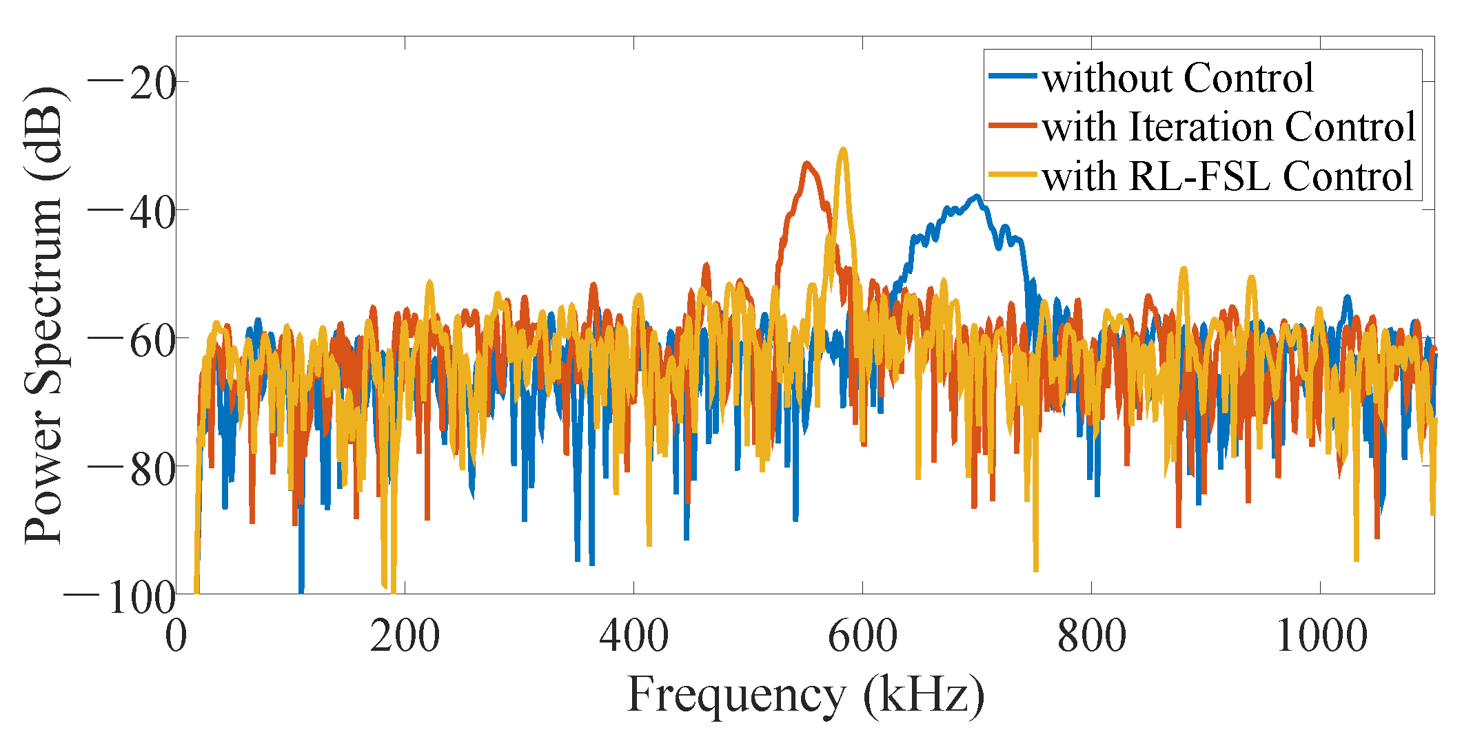According to Equation (2), it means a much smaller RMSRN verifying the effectiveness of our RL-FSL. With the power spectrum analysis shown in Figure 7, it is obvious that, compared to the case without control, the frequency components contained in the beat signals are reduced and the proposed RL-FSL is better than the iteration method. The bandwidth of the beat signal with the control of our RL-FSL method is 5.6 kHz, which is an order of magnitude improvement compared to 59.2 kHz without linearization. And, the bandwidth based on the iteration method is 19.8 kHz. Considering the Equation (10), we can approximate the corresponding RMSRN as 57.3 MHz, 910.3 MHz, and 283.3 MHz, respectively, which represents a significant improvement of the linearity by using our data-driven method. Since the aim of the RL-FSL is to learn long-term reward-maximum behavior, with the proper design of state, action, and reward, the linearization task is converted to the MDP and achieves the control policy suitable to the whole sweep period, where the nonlinearity is extremely variable with time. However, the performance of the iteration method is not good enough in this broadband frequency-swept linearization task. Because of the inherent randomness of the system and the little concern of the influence among different time steps, it is quite difficult to obtain a stable control policy with the iteration method, which would affect the performance of linearization accordingly. Since the principle of the nonlinearity measurement system is similar to the FMCW LiDAR system, we use the beat signal collected in the nonlinearity measurement system as the distance detection result to evaluate the effect of linearization on ranging precision. Based on Equation (11), the best achievable resolution of our method is 0.0072 ml much better than the results without linearization (0.0759 m) and with the iteration method (0.0254 m). Therefore, our proposed RL-FSL would be powerful in the FMCW LiDAR and other application systems.

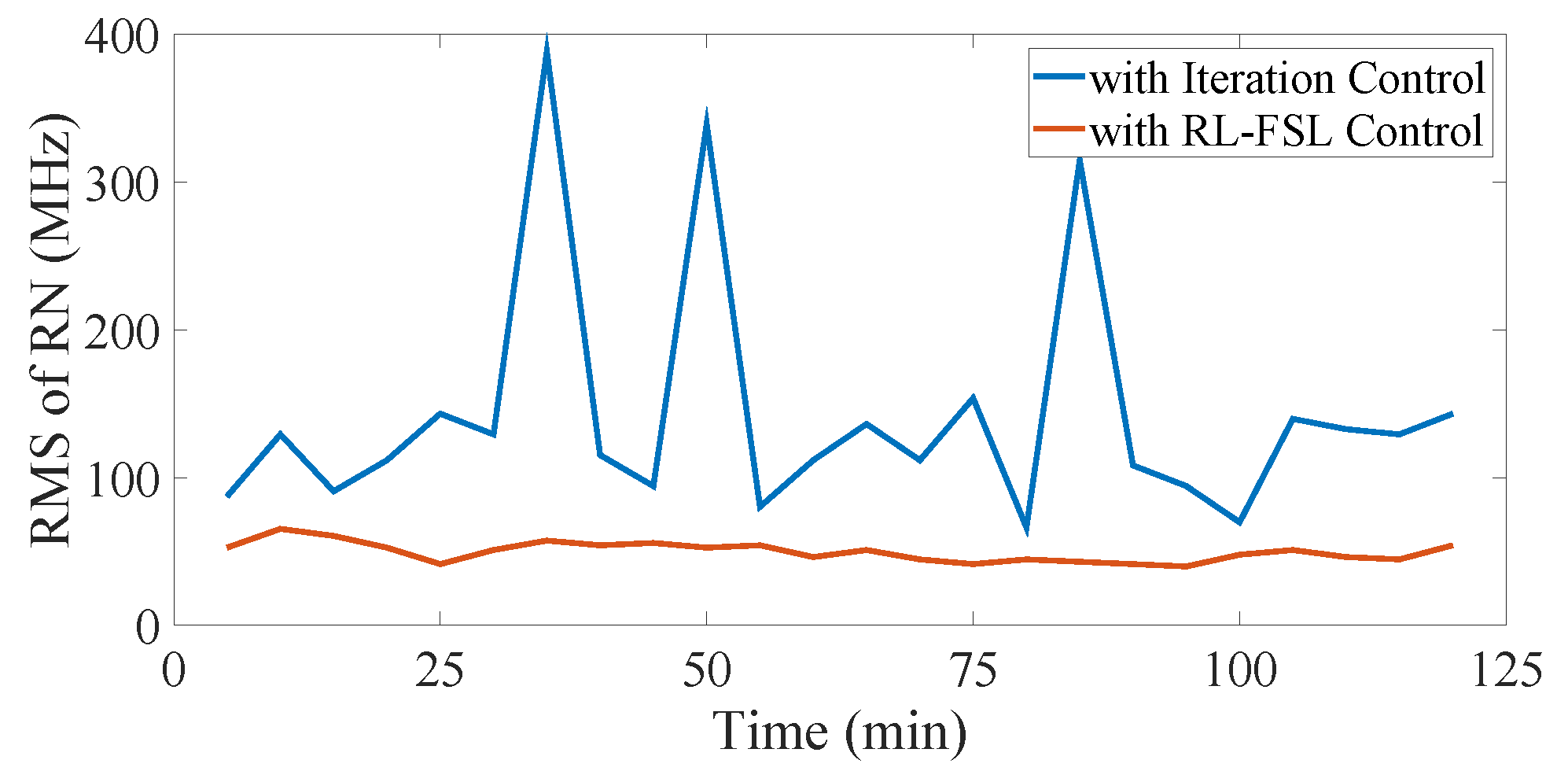
To achieve a stable resolution, it is necessary to monitor the long-term performance of the control methods. As shown in Figure 8, the experimental system operates continuously for over 2 h and the modulation current is updated every 5 min. It is evident that the RMSRN of the beat frequency is larger and highly volatile with the iteration control. It turns out that the iteration process does not make the method robust to the noise of the system, or even worse. On the contrary, the curve of the RMSRN shows small fluctuations over time without degradation, indicating a stable work condition and control efficiency of the RL-FSL methods. Therefore, the established simulator performs good descriptions of the system characteristics and the off-line well-trained control policy performs well in long-term operation, demonstrating the potential of generating the linear frequency-swept signal in the application systems of the FSL without the aid of extra components like the iteration method.

However, since the random term in the system model cannot fully capture the randomness, the linearization performance of the well-trained policy would be influenced if the environment condition changes extremely. In this condition, the system model requires further optimization and the control policy also needs to be re-optimized case-by-case. A few extra training periods are required to fine-tune the agent on the basis of the well-train policy. We would continue to investigate this developing field to generalize our RL algorithm on the variable environments.

Finally, we list the comparison of our proposed RL-FSL with other traditional linearization methods in

Table 1. The comparison of linearization methods.

	Method	Laser	Bandwidth (GHz)	TSR (m)	System Complexity 2
1	EO-PLL [8]	DFB	60	0.005 1	Increase
2	Iteration [12]	DFB	26	0.014 1	Increase
3	Iteration [13]	DFB	36	0.009 1	Increase
4	Ours	DFB	117	0.006	Not increase

¹ The theoretical value calculated with the parameters in the reference papers according to Equations (10) and (11). ² The complexity of the FMCW LiDAR system.

. It can be found that the bandwidth we focus on is much larger than other works. And, the TSR raises to the same magnitude, indicating the potential of our method. The system complexity mentioned in Table 1 is related to the application systems. When the iteration method and the PLL-based method are employed to linearize the frequency-swept laser, the elements including MZI, PD, and the analog digital converter (ADC) are required to set up the application system. Therefore, the system complexity increases. On the contrary, with our proposed RL-FSL, the elements are only needed in the process of simulator establishment. Since the training process of the RL-FSL is accomplished with the interaction of the simulator and the generated modulation current, according to the well-trained policy, is injected to the FSL, the elements mentioned above are not required. Therefore, with the introduction of the data-driven method, the complexity of the application system is under control.

In this work, we have built the nonlinearity measurement system and collected experimental data to establish the system model. With the nonlinear mapping relationship and the random factor concerned, the system model can be effectively utilized as the RL environment. Furthermore, according to the objective of the linearization task and the data characteristics, the task is converted to MDP with the proper definitions of the state, the action, and the reward. Therefore, during the interaction process, the agent is capable of capturing the nonlinear characteristic of the frequency-swept laser. Since the training process is accomplished with a model, the well-trained policy can be applied to the system directly without the iteration process and there is no need to add an auxiliary sub-system for the beat signal measurement in frequency-swept laser application systems, like most traditional methods do. Therefore, the control efficiency is improved and the system complexity is reduced.

Furthermore, RL has more advantages of learning long-term reward-maximizing behavior in high-dimensional control tasks to adapt to the dynamic environment very well. Therefore, rather than traditional methods, such as the iteration methods and PLL-based methods, considering the frequency difference at each time step separately, the RL agent has a better performance of learning the nonlinear characteristics of the environment.

Moreover, the broadband frequency sweep leads to the enhanced nonlinearity and an extreme increase in the dimensions of the state and action spaces in the environment. The NN structure makes it possible to further mine the experimental data to reflect the system. The proper designed actor NNs do well in optimizing the deterministic control policy. And, the critic NNs estimate the state-action value function to evaluate the current policy.

With the well-trained policy, the modulation current is generated during the interaction of the agent and the environment, and applied to the experiment system to evaluate the linearization ability of the control policy. Due to the random terms present in the environment, the generated modulation signals are slightly different in different modulation periods. Therefore, our generated modulation current is flexible enough to accommodate the random changes in the model. By updating the modulation current regularly, the linearity of the system has a better performance faced with random changes of the system.

Therefore, the control efficiency is improved and the system complexity is reduced by using the data-driven RL-FSL. More generally, similarly to the frequency-swept laser control, many optical phenomena in optical systems are also noise-sensitive, high-dimensional, and nonlinear, making it challenging to use conventional control methods. Therefore, the data-driven method has the potential to drive the development of smart photonics technologies.

4. Conclusions

In this work, we linearized the broadband FSL with an RL algorithm. The nonlinearity of the FSL is characterized and simulated by the experimental data. And, the NNs fully explored the hidden characteristic in the data, ensuring the data efficiency. Simultaneously, the establishment of the nonlinearity measurement system and the off-line training made the optimization process of the control policy decoupled from the actual application effectively alleviating the system complexity of the actual application. The RMSRN reduced by 15 times demonstrated the advantages of the data-driven method in broadband frequency-swept linearization, compared with traditional methods. For FMCW LiDAR, it means an order of magnitude of resolution improvement. And, it could also be implemented to enhance the performance in a wide variety of applications, including optical fiber sensor networks for remote sensing, spectroscopy, and so on.