Abstract
In this work, we consider an environment formed by incoherent photons as a resource for controlling open quantum systems via an incoherent control. We exploit a coherent control in the Hamiltonian and an incoherent control in the dissipator which induces the time-dependent decoherence rates (via time-dependent spectral density of incoherent photons) for generation of single-qubit gates for a two-level open quantum system which evolves according to the Gorini–Kossakowski–Sudarshan–Lindblad (GKSL) master equation with time-dependent coefficients determined by these coherent and incoherent controls. The control problem is formulated as minimization of the objective functional, which is the sum of Hilbert-Schmidt norms between four fixed basis states evolved under the GKSL master equation with controls and the same four states evolved under the ideal gate transformation. The exact expression for the gradient of the objective functional with respect to piecewise constant controls is obtained. Subsequent optimization is performed using a gradient type algorithm with an adaptive step size that leads to oscillating behaviour of the gradient norm vs. iterations. Optimal trajectories in the Bloch ball for various initial states are computed. A relation of quantum gate generation with optimization on complex Stiefel manifolds is discussed. We develop methodology and apply it here for unitary gates as a testing example. The next step is to apply the method for generation of non-unitary processes and to multi-level quantum systems.
1. Introduction
Optimal control of quantum systems has various applications ranging from quantum computing to optimal molecule discrimination [1,2,3,4,5]. Often controlled quantum systems are interacting with the environment. Hence, they have to be considered as open quantum systems. In some situations, the environment prevents from controlling the system. In other cases, it can be used as a useful resource. An example is via incoherent control proposed in [6,7], where time dependent decoherence rates induced by non-equilibrium spectral density of incoherent photons are generally used as control jointly with coherent control by lasers. This incoherent control uses the engineered environment as a useful resource. Such incoherent control was applied to general multilevel systems in the dynamical picture (i.e., using master equations for the description of the dynamics) [8], as well as to specific problems for single-qubit and two-qubit models, e.g., in [9,10,11,12], etc. Controllability of open quantum systems in the kinematic picture (using universally optimal Kraus maps for description of evolution of the system) was studied in [13]. The first experimental realization of Kraus maps studied in [13] for an open single qubit was done in [14].
Engineered environments were used for manipulation of quantum systems in various contexts. Preparation of mixed states and generation of non-unitary evolutions are necessary for quantum computing with mixed states and non-unitary circuits [15,16]. Engineered environments were suggested for improving quantum state engineering [17], cooling of translational motion without reliance on internal degrees of freedom [18], preparing entangled states [19,20], improving quantum computation [17], inducing multiparticle entanglement dynamics [21], and making robust quantum memories [22]. A scheme for steady-state preparation of a harmonic oscillator in the first excited state using dissipative dynamics was proposed [23]. Quantum harmonic oscillator state preparation by reservoir engineering was considered [24]. Optimal control for cooling a quantum harmonic oscillator by controlling its frequency was proposed [25]. Reachable states for a qubit driven by coherent and incoherent controls were analytically described using geometric control theory [10]. Controllability analysis of quantum systems immersed within an engineered environment was performed [26]. Coherent control and simplest switchable noise on a single qubit were shown to be capable of transferring between arbitrary n-qubit quantum states [27]. Quantum state preparation by controlled dissipation in finite time was proposed [28]. Precision limits to quantum metrology of open dynamical systems through environment control were studied [29].
Various optimization methods are used to find controls for quantum systems including Krotov type approaches ([30,31,32], Zhu–Rabitz [33] method, GRadient Ascent Pulse Engineering (GRAPE) [34], Hessian based optimization in the Broyden–Fletcher–Goldfarb–Shanno (BFGS) algorithm and combined approaches [35,36], speed gradient method [37], gradient free Chopped RAndom Basis (CRAB) optimization [38], genetic algorithms [6,39], dual annealing [11], machine learning [40], etc. Quantum speed limit for a controlled qubit moving inside a leaky cavity has been studied [41]. Preparation of single qubit and two-qubit gates has been studied, e.g., in [32,42,43,44,45,46,47,48,49], etc.
In this work, the incoherent control in the dissipator is implemented using the environment formed by incoherent photons and is used as a resource, together with the coherent control in the Hamiltonian, to control a single qubit system, based on the approach in [6]. The incoherent control induces time-dependent decoherence rates via time-dependent spectral density of the environment , in addition to the coherent control. The following master equation for the system density matrix evolution was proposed [6]:
Here, is a free system Hamiltonian, is a Hamiltonian describing interaction of the system with coherent control, k denotes all possible different pairs of energy levels in the system, and is a Gorini–Kossakowski–Sudarshan–Lindblad (GKSL) dissipator (we set Planck constant as ). In addition to general consideration, two physical classes of the environment were exploited in [6]—incoherent photons and quantum gas, with two explicit forms of derived in the weak coupling limit (describing atom interacting with photons) and low density limit (describing collisional type decoherence), respectively. In [8], it was shown that for the master equation (1) with derived in the weak coupling limit, a generic N-level quantum system becomes approximately completely controllable in the set of density matrices.
As particular control example, we consider here generation of the single-qubit gate X (Pauli matrix X) and Hadamard gate H for a two-level open quantum system, evolving according to the Gorini–Kossakowski–Sudarshan–Lindblad master equation with time-dependent coefficients determined by these coherent and incoherent controls. The control problem is formulated as the minimization of the objective functional, which is the sum of Hilbert–Schmidt distances between density matrices evolving under controls from some basis states for some time T and target density matrices. The target density matrices are produced from the basis states using the ideal quantum gate. Note that using three specific mixed states is enough in the general case of a N-level quantum system [32]. We obtain an exact expression for the gradient of the objective functional with respect to piecewise constant controls and perform the optimization using a gradient type algorithm with an adaptive step size. The use of the adaptive step size leads to oscillating behavior of the norm of the gradient vs. number of iterations, which is in contrast to Figure 2 in [50]. In that figure, the norm of the gradient of the objective first monotonically increases, and then, monotonically decreases with number of the iterations. We visualize the results by plotting in the Bloch ball evolution of the initial states under obtained controls which are in a good agreement with the ideal case.
We utilize the gradient descent method for optimization. In the context of quantum control, it is known as GRAPE. The gradient descent is a local method and does not necessarily converge to a global minimum. It can converge to a local minimum if such a local minimum exists. Therefore, for objective functionals with traps, i.e., local but not global minima, using slower global stochastic methods might be preferable. The analysis of traps for quantum systems was initiated in [51] and studied for various models in [50,52,53,54,55,56,57,58,59,60], etc.
The analysis of this work is related to the approach developed in [61,62] to control of open quantum systems, where Kraus maps are described by points of a complex Stiefel manifold (strictly speaking, factor of the Stiefel manifold over some equivalence relation). This picture is called a kinematic picture for description of the dynamics. In these works, the gradient and Hessian based optimization methods were developed for optimization of control objectives for open quantum systems. In the present work, we consider the dynamical picture, where evolution of an open qubit is described by a master equation. The relation between the two approaches is that this master equation induces some time evolved Kraus map, which corresponds to some trajectory on a suitable factor of a Stiefel manifold. The gradient of the objective in the dynamic picture, which is used to find optimal controls, can be computed using chain rule for derivatives and gradient of the objective computed in the kinematic picture.
The structure of this paper is the following. In Section 2, the master equation for a qubit driven by coherent and incoherent photons is provided. In Section 3, incoherent control by photons is discussed in more details. In Section 4, the objective functional which describes the problem of generation of single-qubit quantum gates is formulated. In Section 5, the gradient of the objective is computed for piecewise constant controls. In Section 6, numerical optimization results are provided, including plots for optimal coherent and incoherent controls, and for the evolution of the qubit basis states in the Bloch ball under the action of the optimal controls. In Section 7, a connection of the obtained results with gradient optimization over Stiefel manifolds [61,62] is discussed. The conclusions in Section 8 summarizes the results.
2. Master Equation for a Qubit Driven by Coherent and Incoherent Controls
We consider a master equation for an open two-level quantum system (qubit) driven by coherent and incoherent controls with time-dependent decoherence rate determined by , where is the spectral density of incoherent photons surrounding the qubit at the time t:
Here, is the free Hamiltonian, is the interaction Hamiltonian, is the transition frequency, is the dipole moment, is coherent control (real-valued function), and is the decoherence rate coefficient. The dissipative superoperator is
where is incoherent control (non-negative real-valued function), matrices , , , and , , are the Pauli matrices.
We use convenient parameterization of the density matrix by Bloch vector :
where is the identity matrix. In this representation, we obtain the following equation for the dynamics of the Bloch vector :
where , and
3. Incoherent Control
Incoherent control as proposed in [6] is realized by using the environment as a resource to manipulate quantum systems. Physically incoherent control can be realized by using incoherent light and tailoring its distribution in frequency. In this case, control is density of photons with frequency ( is photon momentum and c is the speed of light) and time t. In general, photons have polarization , and their proper distribution should include dependence on polarization, if any, so that incoherent control becomes a function of , , and t. However, we neglect this dependence in the present work. For thermal light or black-body radiation, distribution of its photons has the famous Planck form
where is the inverse temperature (in the Planck system of units, where reduced Planck constant ℏ, speed of light c, and Boltzmann constant equal one). However, it can generally be non-thermal with other shape , which can evolve in time. One can obtain non-thermal shapes, e.g., by filtering of black-body radiation, using light-emission diodes, etc. A plot with Planck distribution and some of its filterings are shown in Figure 1.
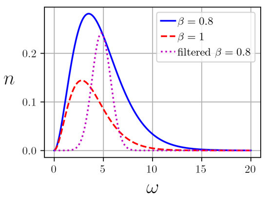
Figure 1.
Planck density of black-body radiation for and Gaussian filtering for centered at with a variance .
Since physical meaning of incoherent control is density of particles of the environment, mathematically, it is a non-negative quantity, . In general, one can require that
meaning that total density of photons at any time moment is finite. Decoherence rates for a quantum system, e.g., an atom, interacting with incoherent light, are determined by strength of interaction between the atom and light, and by this density of photons. Such incoherent control naturally makes decoherence rates time dependent. The magnitude of the decoherence rates affects the speed of decay of off-diagonal elements of the system density matrix and determines the values of the diagonal elements towards which the diagonal part of the system density matrix evolves. This property can be used, for example, for approximate generation of various density matrices [8].
In our case of a single qubit, the qubit only has one transition frequency . In the first approximation, the spectral density of incoherent light at only this frequency, , affects the system. Thus, in this case, without loss of generality, one can use only thermal radiation with variable temperature. For multilevel systems, this is not the case and thermal distribution with variable temperature does not provide the full generality for incoherent control at all system’s transition frequencies.
4. Objective Functional for Single-Qubit Gate Generation
Let us introduce the evolution superoperator , also called as dynamical map, which is a completely positive and trace preserving superoperator. The evolution superoperator acts on the initial density matrix and maps it to the solution of the system (2) evolving under controls u and n for :
To find a control that steers the initial state to the target state as close as possible, one can use the Hilbert–Schmidt distance
and solve the optimal control problem of finding controls u and n which minimize the objective functional
It should be noted that there might be many different controls that steer the system to the given target state.
Generation of a unitary quantum gate U means that we are looking for controls u and n which produce the evolution operator that is close enough to the “target” dynamic map . Hence, we need to use a functional which will describe similarity of two dynamic maps. Let , be the basis density matrices in the space of density matrices. Two linear maps coincide if they act identically on the basis. Therefore, the following functional can be used to compare two dynamic maps and :
Hence, for gate generation, we consider the objective functional
Now, we formulate this problem using the Bloch parameterization. Make the correspondence between density matrices and vectors in the Bloch ball as
Then, the problem (9) is formulated as
It can be seen that values of the objective functional (12) are bounded, both below and above, as
Finding exact maximum and minimum values for a fixed time T, basis and gate U is not a trivial problem.
We use initial pure states , , which form a basis in the linear space of Hermitian matrices, to define action of the unitary gate U:
Here, are pure state density matrices formed by eigenvectors of Pauli matrices (vectors and ), (vector ), and (vector ). Note that, as was mentioned in the Introduction, three special mixed states are enough in the general case of a quantum system of an arbitrary dimension [32].
Any single-qubit initial density matrix can be uniquely decomposed in the basis (13):
Therefore, this number of states is sufficient to define any linear operator: particularly, any unitary transformation . The corresponding Bloch vectors are
We also consider the objective functional with only two states and to show that this system is insufficient for generating quantum gates. Indeed, the quantum gate (rotation along y-axis by angle in the Bloch ball) acts exactly as the Hadamard gate H on the states and :
However, these two gates are different.
5. Gradient of the Objective Functional
The main features of quantum control landscape are local (if they exist) and global extrema of the objective functional. Since extrema are critical points where gradient of the objective is zero, an important step for the analysis of quantum control landscapes is the derivation of the expression for gradient of the objective. Below, we derive the gradient for piecewise constant control. Incoherent control is constrained: ; therefore, we make a variable change:
so that control becomes a pair of u and w. The controls, and , as piecewise constant functions, are defined by M-dimensional real vectors and :
where and is the characteristic function of the half-open interval . For the sake of brevity, we denote this pair as and its components as , .
The solution of the equation with piecewise constant r.h.s can be expressed using the following recurrent formula:
where
Differentiating the final state (21) with respect to the kth component of piecewise constant controls u (19) and w (20) gives
The derivatives are given by
The expressions (25) and (27) were found using the integral formula [63]:
Finally, the derivatives of the functional (12) with respect to the components and of the controls u and w, respectively, are
6. Numerical Optimization for Generation of and Gates
In this section, we use the above derived gradient (29) of the objective function to implement a gradient optimization method for generating single-qubit quantum gates. We consider two single-qubit gates: the X gate, which is Pauli matrix, and the Hadamard gate H, i.e., :
To find controls u (19) and w (20) that minimize the objective functional (12), we utilize the gradient descent method known in the context of quantum control as GRAPE. This is an iterative algorithm, where each update of the control describes moving against the gradient of the objective functional:
Here, for brevity, we denote
where the basis matrices are fixed and chosen as (13), their Bloch representations are given by (15); denotes a -dimensional vector operator, each of the components acts according to formula (23); is the control on the lth iteration; and is the size of the lth step.
The stopping criterion is the condition for the fidelity to be small enough, such that fidelity value on the lth step is less than some precision parameter :
This stopping criterion is satisfied when we find an optimal control that steers the initial basis states to the final states that are different from the action of the unitary gate U on them, , less than in the sense of mean square of the Hilbert–Schmidt distances (9). Since each control defines some dynamical map on the space of density matrices, we attempt to construct a dynamical map which is as close as possible to the desired map produced by the target quantum gate U.
Performance of gradient descent (31) largely depends on the choice of a step size sequence . Often with a predefined sequence , gradient descent method may produce a fidelity value sequence which is not monotonically decreasing. We propose the adaptive choice of step size and modification of the control update rule (31). In each th iteration, we compute the potential next updated value of fidelity and compare it with the last value on the lth iteration ; if it is lower, we update the control; otherwise, the control and the fidelity value remain the same:
Increase of the fidelity means that the step size is too large; therefore, we decrease the next step in the second case. We also increase the step size in the first case to boost up the gradient descent:
where ,
Thus, we produce a monotonically (not strictly) decreasing sequence of fidelity values . This scheme allows us to adapt step size to the local change of the functional landscape. This approach may significantly reduce the number of iterations needed to reach the desired accuracy of optimization. The adaptive scheme (35) depends on the three parameters, which were chosen as: , , .
The important question is whether the adaptive scheme (34) and (35) may stuck in a non-critical point x (i.e., in a point with gradient ), i.e., may constantly reduce size of the step without decrease of the objective functional. If gradient is calculated with absolute precision, there would exist a step size h which is sufficient to decrease the value of the objective functional. This intuitive statement can be proved by the following simple reasoning. Consider a differentiable functional . Then, in a vicinity of an internal point :
Due to the definition of , for any , there exists such that . If x is not a critical point (so that ), we can take and . Thus, the answer to the posed question is “no”—after a finite number of iterations (35), the step size will be small enough to decrease the objective functional value. However, practice of numerical experiments shows that the adaptive scheme sometimes does not provide the objective functional value decrease over quite large number of iterations. In order to deal with such cases, we utilize one more stop criterion. The second criterion is the following: if , the iterations also are stopped. We set as the maximum number of “stationary” iterations.
Numerical computations were performed by writing a Python program with the use of the Numpy library for fast matrix operations and the SciPy library function scipy.linalg.expm for matrix exponentials computation using the Padé approximation. The following values of the system parameters were used: the transition frequency , the dipole moment , and the decoherence rate coefficient . We use regular partition of the time segment with into segments, such that each segment has length . Integral formulae were approximated by the trapezoidal rule with the number of partitions .
Initial guesses for a coherent control and for an incoherent control were chosen as discretization of the sine function and the normal distribution function (similar to physical realization of coherent and incoherent controls): , . The precision parameter was .
Figure 2 illustrates optimized coherent (subplot a) and incoherent controls (subplot b) for generating the gate X (blue line) and the Hadamard gate H (purple line), convergence of the fidelity—the objective functional , (33) (subplot c)—and norm of the gradient of the objective functional (subplot d) vs. number l of the optimization algorithm (31) iterations under the optimized coherent and incoherent controls. As shown on subplot (a), for generation of H gate, the fidelity goes to a small value of in about 30 iterations. For this gate, the convergence is fast. For generation of X gate, the convergence to such a low value of the fidelity is much slower; even after 120 iterations, the fidelity is still slightly above this value. Thus, high-precision generation of X gate is more difficult with the present gradient approach. For Hadamard gate, which is found to be easily generated with this approach, higher (compared to the case of X gate) values of incoherent control were obtained, as shown on subplot (b). The difference of scales is large, since our target in this analysis is a unitary gate, and as confirmed by the plots, it is natural to expect that incoherent control, while non-trivial, will have much smaller values than coherent. These gates are good testing examples and the results are in the agreement with expectation. The next step will be to apply the method for generation of target non-unitary processes, where incoherent control component should be more significant, as was found before for the problem of mixed state generation [11]. Coherent controls, which were found here as the results of optimization, for X and H gates are to some degree symmetric around a constant value .
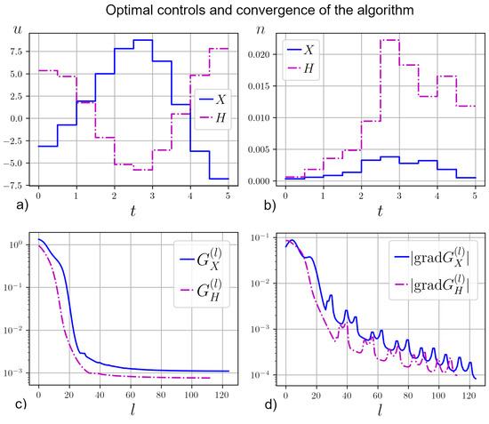
Figure 2.
Optimized coherent control (subplot a) and incoherent control (subplot b) which generate the quantum gate X (blue line) and the Hadamard quantum gate H (purple line); convergence of the fidelity—the objective functional (33)—(subplot c); norm of the gradient of the objective functional (subplot d) vs. number l of the optimization algorithm (31) iterations.
Figure 3 shows optimal trajectories of the basis states (15) in the Bloch ball for generation of the quantum gate X (subplot a) and the Hadamard quantum gate H (subplot b), where four initial states, corresponding to () are indicated by green dots, final states by red squares, and target states are centers of the black circles. Optimal trajectories are very close to the Bloch sphere (the longest distance to the sphere is up to ). However, they are located in the interior of the Bloch ball due to unavoidable non-unitary evolution of the system and the presence of incoherent control.
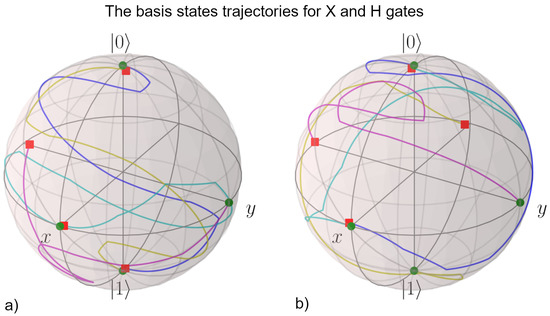
Figure 3.
Optimal trajectories of the basis states (15) in the Bloch ball for generation of the quantum gate X (subplot a) and the Hadamard quantum gate H (subplot b). Initial states are indicated by green dots, final states by red squares, and target states are centers of the black circles. The trajectories lie close to the Bloch sphere, in the region with a distance of about to the sphere.
We note that on Figure 3, the norm of the gradient has oscillating behavior vs. number of iterations. This is in contrast to the case of [50] (see Figure 2 in that paper), where the norm of the gradient of the objective first monotonically increases, and then, monotonically decreases with the number of iterations. This difference in the behavior is expected to be due to the adaptive step size used in the present work.
7. Discussion: Quantum Gate Generation as Optimization over Complex Stiefel Manifolds
Our analysis in this work is directly related to the gradient optimization approach which was developed for open quantum systems using a proposed formulation of completely positive trace preserving dynamics of open quantum systems as points of complex Stiefel manifold (rigorously speaking, as points in quotient space of complex Stiefel manifolds over some equivalence relation). The corresponding theory of gradient optimization over complex Stiefel manifolds was developed for two-level [61] and general N–level quantum systems [62].
Recall that the dynamics of density matrix of an N-level open quantum system can be described as a completely positive trace preserving map (Kraus map), which has an operator sum representation
where are complex matrices such that
and is the identity operator. Denote matrix
The condition (36) is equivalent to
The set of matrices which satisfy this condition forms a complex Stiefel manifold , which is the set of all orthonormal N-frames in . As is well known, a given physical evolution (Kraus map) has a non-unique Kraus map operator-sum representation. Thus, different sets of may describe the same physical evolution and one should take the appropriate equivalence class . This equivalence was taken into account in [62]. In particular, the Hadamard gate corresponds to the matrix
which is a point of the complex Stiefel manifold .
Coherent and incoherent controls which act on our one-qubit system (and more generally, on any quantum system) induce some time evolving Kraus map , which induces some trajectory on the Stiefel manifold. Thus, optimization of gate generation can be formulated as optimization over complex Stiefel manifold. The corresponding theory, including gradient and Hessian-based optimization, in the kinematic picture was developed in [61,62]. In our example, optimal controls plotted on Figure 2 induce some trajectory on the Stiefel manifold. Since the dimension of the manifold is , the corresponding evolution can not be drawn as one can draw for evolution of single-qubit states on the Bloch ball, but the Stiefel matrices for any moment in time can be computed.
8. Conclusions
In this work, we have exploited the coherent control and the environment formed by incoherent photons as a resource for generation of single-qubit gates in a two-level open quantum system evolving according to the Gorini–Kossakowski–Sudarshan–Lindblad master equation with time-dependent coefficients. The coherent control enters in the Hamiltonian, and the incoherent control enters in the dissipator and induces time-dependent decoherence rates of the system. The exact expression for the gradient of the objective functional with respect to piecewise constant controls has been obtained, and the optimization has been performed using the gradient type algorithm. The optimal coherent and incoherent controls and the basis states trajectories in the Bloch ball have been computed. The numerical optimization shows that generation of the H gate is fast (a value of is obtained in about 30 iterations), giving low values of fidelity. For the X gate optimization, it takes a much higher number of iterations (120 iterations were not enough). Thus, high-precision generation of X gate is more difficult with the present approach, that might be due to the limits of controllability of the system [10]. For the Hadamard gate, higher values of incoherent control were obtained, compared to the case of the X gate. The coherent controls, obtained as the results of optimization for X and H gates, are found to some degree to be symmetric around a constant value . In this work, we use the adaptive step size of the gradient search to analyze the landscape. This leads to oscillating behavior of the norm of the gradient vs. number of iterations; this contrasts Figure 2 in [50], where the norm of the gradient of the objective firstly monotonically increases, and then, monotonically decreases with the number of iterations. While we use the particular model for the dissipative superoperator, the approach can be extended to other cases as well. Here, we develop the theoretical basis of the approach and apply it for target unitary gates as a testing example. In this case, the incoherent control magnitude is obviously small. The next step is to apply the method for generation of target non-unitary processes, where incoherent control component should be more significant, as was found before for the problem of mixed state generation [11].
Author Contributions
Conceptualization, A.N.P.; methodology, V.N.P. and A.N.P.; formal analysis, V.N.P. and A.N.P.; writing, V.N.P. and A.N.P.; visualization, V.N.P.; supervision, A.N.P.; project administration, A.N.P.; discussion, A.N.P., funding acquisition, A.N.P. All authors have read and agreed to the published version of the manuscript.
Funding
The new results in Section 3, Section 4, Section 5 and Section 6 were obtained in Steklov Mathematical institute and supported by Russian Science Foundation under grant No. 22-11-00330, https://rscf.ru/en/project/22-11-00330/ (accessed on 3 January 2023), and in Section 7 in the University of Science and Technology MISIS under the federal academic leadership program “Priority 2030” (MISIS Grant No. K2-2022-025).
Institutional Review Board Statement
Not applicable.
Informed Consent Statement
Not applicable.
Data Availability Statement
Not applicable.
Conflicts of Interest
The authors declare no conflict of interest.
Abbreviations
The following abbreviations are used in this manuscript:
| GKSL | Gorini–Kossakowski–Sudarshan–Lindblad |
| GRAPE | GRadient Ascent Pulse Engineering |
References
- Koch, C.P.; Boscain, U.; Calarco, T.; Dirr, G.; Filipp, S.; Glaser, S.J.; Kosloff, R.; Montangero, S.; Schulte-Herbrüggen, T.; Sugny, D.; et al. Quantum optimal control in quantum technologies. Strategic report on current status, visions and goals for research in Europe. EPJ Quantum Technol. 2022, 9, 19. [Google Scholar] [CrossRef]
- Tannor, D.J. Introduction to Quantum Mechanics: A Time Dependent Perspective; University Science Books: Sausilito, CA, USA, 2007. [Google Scholar]
- Brif, C.; Chakrabarti, R.; Rabitz, H. Control of quantum phenomena: Past, present and future. New J. Phys. 2010, 12, 075008. [Google Scholar] [CrossRef]
- Moore, K.W.; Pechen, A.; Feng, X.J.; Dominy, J.; Beltrani, V.J.; Rabitz, H. Why is chemical synthesis and property optimization easier than expected? Phys. Chem. Chem. Phys. 2011, 13, 10048–10070. [Google Scholar] [CrossRef] [PubMed]
- D’Alessandro, D. Introduction to Quantum Control and Dynamics, 2nd ed.; Chapman & Hall/CRC: New York, NY, USA, 2021. [Google Scholar]
- Pechen, A.; Rabitz, H. Teaching the environment to control quantum systems. Phys. Rev. A 2006, 73, 062102. [Google Scholar] [CrossRef]
- Pechen, A. Incoherent light as a control resource: A route to complete controllability of quantum systems. arXiv 2012, arXiv:1212.2253. [Google Scholar]
- Pechen, A. Engineering arbitrary pure and mixed quantum states. Phys. Rev. A 2011, 84, 042106. [Google Scholar] [CrossRef]
- Morzhin, O.V.; Pechen, A.N. Minimal time generation of density matrices for a two-level quantum system driven by coherent and incoherent controls. Int. J. Theor. Phys. 2021, 60, 576–584. [Google Scholar] [CrossRef]
- Lokutsievskiy, L.; Pechen, A. Reachable sets for two-level open quantum systems driven by coherent and incoherent controls. J. Phys. A Math. Theor. 2021, 54, 395304. [Google Scholar] [CrossRef]
- Morzhin, O.; Pechen, A. Generation of density matrices for two qubits using coherent and incoherent controls. Lobachevskii J. Math. 2021, 42, 2401–2412. [Google Scholar] [CrossRef]
- Petruhanov, V.N.; Pechen, A.N. Optimal control for state preparation in two-qubit open quantum systems driven by coherent and incoherent controls via GRAPE approach. Int. J. Mod. Phys. A 2022, 37, 2243017. [Google Scholar] [CrossRef]
- Wu, R.; Pechen, A.; Brif, C.; Rabitz, H. Controllability of open quantum systems with Kraus-map dynamics. J. Phys. A Math. Theor. 2007, 40, 5681–5693. [Google Scholar] [CrossRef]
- Zhang, W.; Saripalli, R.; Leamer, J.; Glasser, R.; Bondar, D. All-optical input-agnostic polarization transformer via experimental Kraus-map control. Eur. Phys. J. Plus 2022, 137, 930. [Google Scholar] [CrossRef]
- Aharonov, D.; Kitaev, A.; Nisan, N. Quantum circuits with mixed states. arXiv 1998, arXiv:quant-ph/9806029. [Google Scholar]
- Tarasov, V.E. Quantum computer with mixed states and four-valued logic. J. Phys. A Math. Gen. 2002, 35, 5207. [Google Scholar] [CrossRef]
- Verstraete, F.; Wolf, M.M.; Cirac, J.I. Quantum computation, quantum state engineering, and quantum phase transitions driven by dissipation. Nat. Phys. 2009, 5, 633. [Google Scholar] [CrossRef]
- Schmidt, R.; Negretti, A.; Ankerhold, J.; Calarco, T.; Stockburger, J.T. Optimal control of open quantum systems: Cooperative effects of driving and dissipation. Phys. Rev. Lett. 2011, 107, 130404. [Google Scholar] [CrossRef]
- Diehl, S.; Micheli, A.; Kantian, A.; Kraus, B.; Büchler, H.P.; Zoller, P. Quantum states and phases in driven open quantum systems with cold atoms. Nat. Phys. 2008, 4, 878–883. [Google Scholar] [CrossRef]
- Weimer, H.; Müller, M.; Lesanovsky, I.; Zoller, P.; Büchler, H.P. A Rydberg quantum simulator. Nat. Phys. 2010, 6, 382–388. [Google Scholar] [CrossRef]
- Barreiro, J.T.; Schindler, P.; Ghne, O.; Monz, T.; Chwalla, M.; Roos, C.F.; Hennrich, M.; Blatt, R. Experimental multiparticle entanglement dynamics induced by decoherence. Nat. Phys. 2010, 6, 943–946. [Google Scholar] [CrossRef]
- Pastawski, F.; Clemente, L.; Cirac, J.I. Quantum memories based on engineered dissipation. Phys. Rev. A 2011, 83, 012304. [Google Scholar] [CrossRef]
- Børkje, K. Scheme for steady-state preparation of a harmonic oscillator in the first excited state. Phys. Rev. A 2014, 90, 023806. [Google Scholar] [CrossRef]
- Kienzler, D.; Lo, H.-Y.; Keitch, B.; de Clercq, L.; Leupold, F.; Lindenfelser, F.; Marinelli, M.; Negnevitsky, V.; Home, J.P. Quantum harmonic oscillator state synthesis by reservoir engineering. Science 2015, 347, 53–56. [Google Scholar] [CrossRef] [PubMed]
- Salamon, P.; Hoffmann, K.H.; Tsirlin, A. Optimal control in a quantum cooling problem. Appl. Math. Lett. 2012, 25, 1263–1266. [Google Scholar] [CrossRef]
- Grigoriu, A.; Rabitz, H.; Turinici, G. Controllability analysis of quantum systems immersed within an engineered environment. J. Math. Chem. 2012, 51, 1548–1560. [Google Scholar] [CrossRef]
- Bergholm, V.; Schulte-Herbrüggen, T. How to transfer between arbitrary n-qubit quantum states by coherent control and simplest switchable noise on a single qubit. arXiv 2012, arXiv:1206.4945. [Google Scholar]
- Baggio, G.; Ticozzi, F.; Viola, L. Quantum state preparation by controlled dissipation in finite time: From classical to quantum controllers. In Proceedings of the 2012 IEEE 51st IEEE Conference on Decision and Control (CDC), Maui, HI, USA, 10–13 December 2012; pp. 1072–1077. [Google Scholar] [CrossRef]
- Davidovich, L.; Taddei, M.M.; Zagury, N.; de Matos Filho, R.L. Quantum metrology of open dynamical systems: Precision limits through environment control. New Dir. Quantum Control. Landsc. 2013, 29, 1–24. [Google Scholar]
- Tannor, D.J.; Kazakov, V.; Orlov, V. Control of photochemical branching: Novel procedures for finding optimal pulses and global upper bounds. In Time-Dependent Quantum Molecular Dynamics; Broeckhove, J., Lathouwers, L., Eds.; Springer: Boston, MA, USA, 1992; pp. 347–360. [Google Scholar] [CrossRef]
- Morzhin, O.V.; Pechen, A.N. Krotov method for optimal control of closed quantum systems. Russ. Math. Surv. 2019, 74, 851–908. [Google Scholar] [CrossRef]
- Goerz, M.H.; Reich, D.M.; Koch, C.P. Optimal control theory for a unitary operation under dissipative evolution. New J. Phys. 2014, 16, 055012. [Google Scholar] [CrossRef]
- Zhu, W.; Rabitz, H. A rapid monotonically convergent iteration algorithm for quantum optimal control over the expectation value of a positive definite operator. J. Chem. Phys. 1998, 109, 385–391. [Google Scholar] [CrossRef]
- Khaneja, N.; Reiss, T.; Kehlet, C.; Schulte-Herbrüggen, T.; Glaser, S. Optimal control of coupled spin dynamics: Design of NMR pulse sequences by gradient ascent algorithms. J. Magn. Reson. 2005, 172, 296–305. [Google Scholar] [CrossRef]
- Dalgaard, M.; Motzoi, F.; Jensen, J.H.M.; Sherson, J. Hessian-based optimization of constrained quantum control. Phys. Rev. A 2020, 102, 042612. [Google Scholar] [CrossRef]
- De Fouquieres, P.; Schirmer, S.; Glaser, S.; Kuprov, I. Second order gradient ascent pulse engineering. J. Magn. Reson. 2011, 212, 412–417. [Google Scholar] [CrossRef] [PubMed]
- Pechen, A.; Borisenok, S.; Fradkov, A. Energy control in a quantum oscillator using coherent control and engineered environment. Chaos Solit. Fractals. 2022, 164, 112687. [Google Scholar] [CrossRef]
- Caneva, T.; Calarco, T.; Montangero, S. Chopped random-basis quantum optimization. Phys. Rev. A 2011, 84, 022326. [Google Scholar] [CrossRef]
- Judson, R.S.; Rabitz, H. Teaching lasers to control molecules. Phys. Rev. Lett. 1992, 68, 1500–1503. [Google Scholar] [CrossRef]
- Dong, D.Y.; Chen, C.L.; Tarn, T.J.; Pechen, A.; Rabitz, H. Incoherent control of quantum systems with wavefunction controllable subspaces via quantum reinforcement learning. IEEE Trans. Syst. Man. Cybern. B Cybern. 2008, 38, 957–962. [Google Scholar] [CrossRef]
- Hadipour, M.; Haseli, S.; Dolatkhah, H.; Haddadi, S.; Czerwinski, A. Quantum speed limit for a moving qubit inside a leaky cavity. Photonics 2022, 9, 875. [Google Scholar] [CrossRef]
- Romero, K.M.F.; Laverde, G.U.; Ardila, F.T. Optimal control of one-qubit gates. J. Phys. A Math. Gen. 2003, 36, 841. [Google Scholar] [CrossRef]
- Grace, M.; Brif, C.; Rabitz, H.; Walmsley, I.A.; Kosut, R.L.; Lidar, D.A. Optimal control of quantum gates and suppression of decoherence in a system of interacting two-level particles. J. Phys. B At. Mol. Opt. Phys. 2007, 40, S103–S125. [Google Scholar] [CrossRef]
- Zhang, T.-M.; Wu, R.-B. Minimum-time control of local quantum gates for two-qubit homonuclear systems. IFAC Proc. Vol. 2013, 46, 359–364. [Google Scholar] [CrossRef]
- Malinovsky, V.S.; Sola, I.R.; Vala, J. Phase-controlled two-qubit quantum gates. Phys. Rev. A 2014, 89, 032301. [Google Scholar] [CrossRef]
- Ghaeminezhad, N.; Cong, S. Preparation of Hadamard gate for open quantum systems by the Lyapunov control method. IEEE/CAA J. Autom. Sin. 2018, 5, 733–740. [Google Scholar] [CrossRef]
- Li, J.-F.; Xin, Z.-X.; Hu, J.-R.; He, D.-H. Quantum optimal control for Pauli operators based on spin-1/2 system. Int. J. Theor. Phys. 2022, 61, 268. [Google Scholar] [CrossRef]
- Hegde, S.S.; Zhang, J.; Suter, D. Toward the speed limit of high-fidelity two-qubit gates. Phys. Rev. Lett. 2022, 128, 230502. [Google Scholar] [CrossRef]
- Jandura, S.; Pupillo, G. Time-optimal two- and three-qubit gates for Rydberg atoms. Quantum 2022, 6, 712. [Google Scholar] [CrossRef]
- Pechen, A.N.; Tannor, D.J. Quantum control landscape for a ∧-atom in the vicinity of second-order traps. Isr. J. Chem. 2012, 52, 467–472. [Google Scholar] [CrossRef]
- Rabitz, H.A.; Hsieh, M.M.; Rosenthal, C.M. Quantum optimally controlled transition landscapes. Science 2004, 303, 1998–2001. [Google Scholar] [CrossRef] [PubMed]
- Pechen, A.N.; Tannor, D.J. Are there traps in quantum control landscapes? Phys. Rev. Lett. 2011, 106, 120402. [Google Scholar] [CrossRef] [PubMed]
- De Fouquieres, P.; Schirmer, S.G. A closer look at quantum control landscapes and their implication for control optimization. Infin. Dimens. Anal. Quantum Probab. Relat. 2013, 16, 1350021. [Google Scholar] [CrossRef]
- Pechen, A.N.; Tannor, D.J. Control of quantum transmission is trap free. Can. J. Chem. 2014, 92, 157–159. [Google Scholar] [CrossRef]
- Larocca, M.; Poggi, P.M.; Wisniacki, D.A. Quantum control landscape for a two-level system near the quantum speed limit. J. Phys. A Math. Theor. 2018, 51, 385305. [Google Scholar] [CrossRef]
- Zhdanov, D.V. Comment on ‘Control landscapes are almost always trap free: A geometric assessment’. J. Phys. A Math. Theor. 2018, 51, 508001. [Google Scholar] [CrossRef]
- Russell, B.; Wu, R.; Rabitz, H. Reply to comment on ‘control landscapes are almost always trap free: A geometric assessment’. J. Phys. A Math. Theor. 2018, 51, 508002. [Google Scholar] [CrossRef]
- Pechen, A.N.; Il’in, N.B. On extrema of the objective functional for short-time generation of single-qubit quantum gates. Izv. Math 2016, 80, 1200–1212. [Google Scholar] [CrossRef]
- Volkov, B.O.; Morzhin, O.V.; Pechen, A.N. Quantum control landscape for ultrafast generation of single-qubit phase shift quantum gates. J. Phys. A Math. Theor. 2021, 54, 215303. [Google Scholar] [CrossRef]
- Dalgaard, M.; Motzoi, F.; Sherson, J. Predicting quantum dynamical cost landscapes with deep learning. Phys. Rev. A 2022, 105, 012402. [Google Scholar] [CrossRef]
- Pechen, A.; Prokhorenko, D.; Wu, R.; Rabitz, H. Control landscapes for two-level open quantum systems. J. Phys. A Math. Theor. 2008, 41, 045205. [Google Scholar] [CrossRef]
- Oza, A.; Pechen, A.; Dominy, J.; Beltrani, V.; Moore, K.; Rabitz, H. Optimization search effort over the control landscapes for open quantum systems with Kraus-map evolution. J. Phys. A Math. Theor. 2009, 42, 205305. [Google Scholar] [CrossRef]
- Wilcox, R.M. Exponential operators and parameter differentiation in quantum physics. J. Math. Phys. 1967, 8, 962. [Google Scholar] [CrossRef]
Disclaimer/Publisher’s Note: The statements, opinions and data contained in all publications are solely those of the individual author(s) and contributor(s) and not of MDPI and/or the editor(s). MDPI and/or the editor(s) disclaim responsibility for any injury to people or property resulting from any ideas, methods, instructions or products referred to in the content. |
© 2023 by the authors. Licensee MDPI, Basel, Switzerland. This article is an open access article distributed under the terms and conditions of the Creative Commons Attribution (CC BY) license (https://creativecommons.org/licenses/by/4.0/).