Fourier Transform Holography: A Lensless Imaging Technique, Its Principles and Applications


Abstract
1. Introduction
1.1. Phase Problem
1.2. Fourier Transform Holography (FTH)
2. Principles of FTH
2.1. Hologram Formation
2.2. Reconstruction of the Sample Distribution from the Hologram
2.3. Optimal Parameters
2.3.1. Distance between the Object and the Reference
2.3.2. The Reconstructed Field of View
2.3.3. The Detector Parameters
2.3.4. Reference Size and Resolution
3. Types of References
3.1. Point-like References
3.1.1. Single Point-like Reference

3.1.2. Multiple Point-like References
3.2. Extended References
3.2.1. References in the Form of Geometrical Shapes

3.2.2. Uniformly Redundant Array (URA) Reference
3.2.3. Arbitrary Extended Reference
3.2.3.1. Reconstruction by Deconvolution
3.2.3.2. Reconstruction via System of Linear Equations
4. FTH with Different Types of Waves
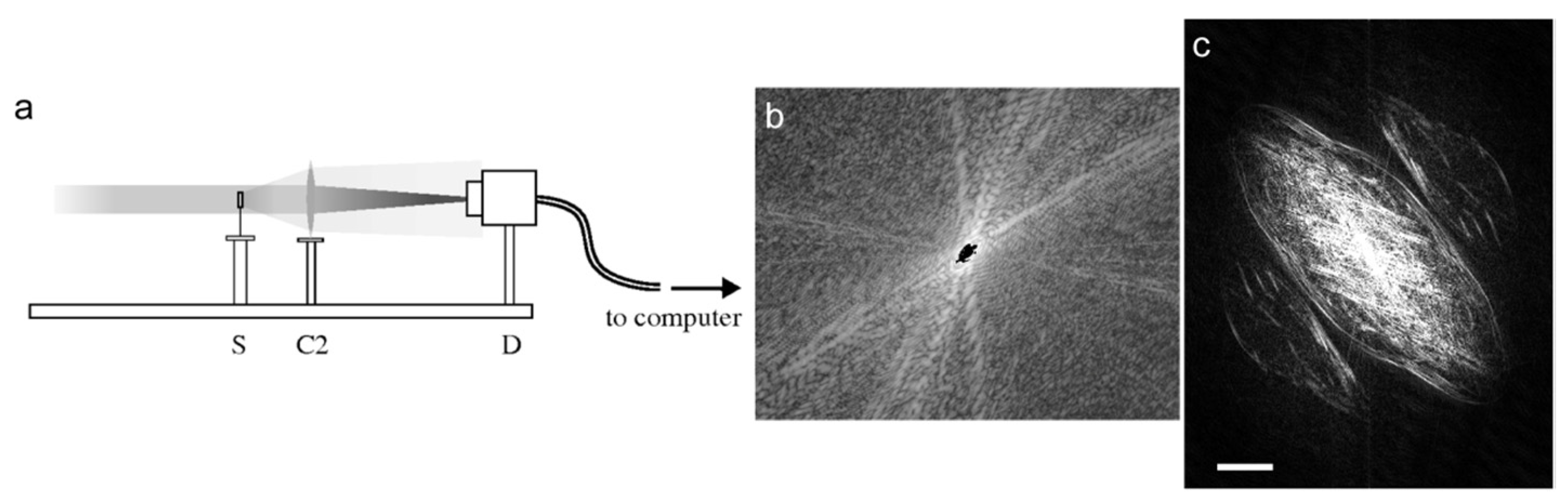
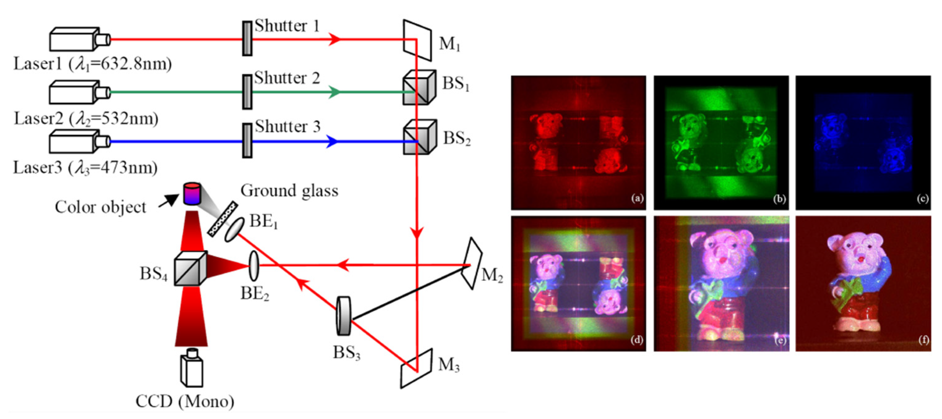
4.1. Light
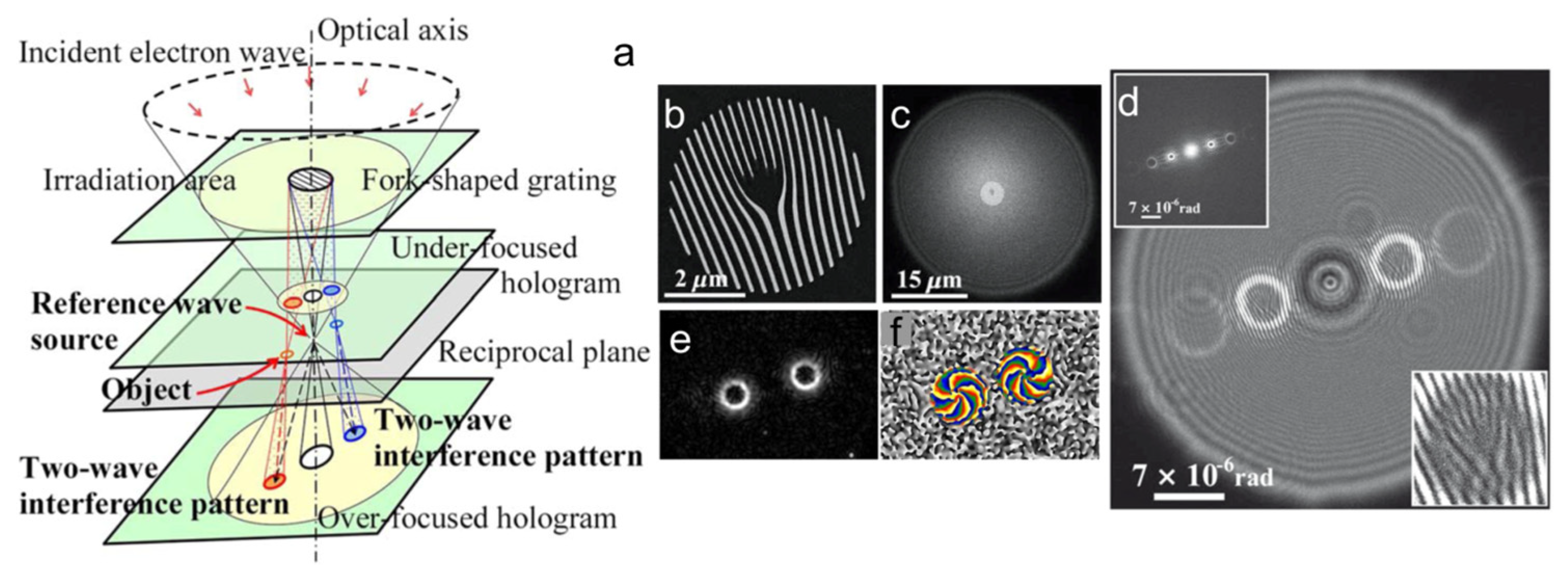
4.2. Electrons
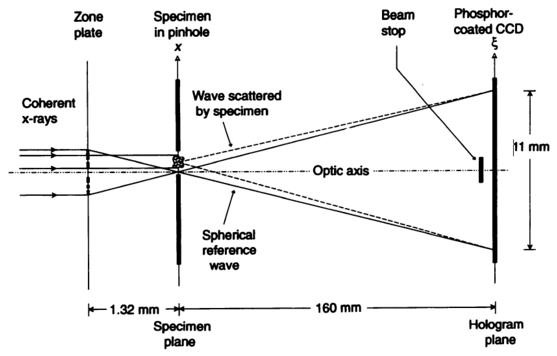
4.3. X-rays and Extreme Ultraviolet
5. X-ray FTH Applications
5.1. Imaging of Magnetic Domains—Spectro-Holography
5.2. Time-Resolved Imaging
5.3. Biological Imaging
5.4. Three-Dimensional Imaging
6. FTH and Other Coherent Imaging Techniques


7. Conclusions
Author Contributions
Funding
Institutional Review Board Statement
Informed Consent Statement
Data Availability Statement
Conflicts of Interest
References
- Gabor, D. Improvements in and Relating to Microscopy. Patent The British Thomson-Houston Company. GB Patent 685,286, 17 December 1947. [Google Scholar]
- Gabor, D. A new microscopic principle. Nature 1948, 161, 777–778. [Google Scholar] [CrossRef] [PubMed]
- Gabor, D. Microscopy by reconstructed wave-fronts. Proc. R. Soc. Lond. A 1949, 197, 454–487. [Google Scholar] [CrossRef]
- Miao, J.W.; Sayre, D.; Chapman, H.N. Phase retrieval from the magnitude of the Fourier transforms of nonperiodic objects. J. Opt. Soc. Am. A 1998, 15, 1662–1669. [Google Scholar] [CrossRef]
- Miao, J.W.; Charalambous, P.; Kirz, J.; Sayre, D. Extending the methodology of X-ray crystallography to allow imaging of micrometre-sized non-crystalline specimens. Nature 1999, 400, 342–344. [Google Scholar] [CrossRef]
- Miao, J.W.; Kirz, J.; Sayre, D. The oversampling phasing method. Acta Crystall. D 2000, 56, 1312–1315. [Google Scholar] [CrossRef]
- Fienup, J.R. Phase retrieval algorithms—A comparison. Appl. Opt. 1982, 21, 2758–2769. [Google Scholar] [CrossRef]
- Shechtman, Y.; Eldar, Y.C.; Cohen, O.; Chapman, H.N.; Miao, J.W.; Segev, M. Phase retrieval with application to optical imaging. IEEE Signal Process. Mag. 2015, 32, 87–109. [Google Scholar] [CrossRef]
- Latychevskaia, T. Iterative phase retrieval in coherent diffractive imaging: Practical issues. Appl. Opt. 2018, 57, 7187–7197. [Google Scholar] [CrossRef]
- Winthrop, J.T.; Worthington, C.R. X-ray microscopy by successive Fourier transformation. Phys. Lett. 1965, 15, 124–126. [Google Scholar] [CrossRef]
- Stroke, G.W. Lensless Fourier-transform method for optical holography. Appl. Phys. Lett. 1965, 6, 201–203. [Google Scholar] [CrossRef]
- Winthrop, J.T.; Worthington, C.R. X-ray microscopy by successive Fourier transformation 2. An optical analogue experiment. Phys. Lett. 1966, 21, 413–415. [Google Scholar] [CrossRef][Green Version]
- Wiener, N. Generalized harmonic analysis. Acta Math. 1930, 55, 117–258. [Google Scholar] [CrossRef]
- Khintchin, A. Korrelationstheorie der stationären stochastischen Prozesse. Math. Ann. 1934, 109, 604–615. [Google Scholar] [CrossRef]
- Debevec, P.E.; Malik, J. Recovering high dynamic range radiance maps from photographs. Siggraph 1997, 130, 1–10. [Google Scholar]
- Thibault, P.; Rankenburg, I.C. Optical diffraction microscopy in a teaching laboratory. Am. J. Phys. 2007, 75, 827–832. [Google Scholar] [CrossRef]
- DeVelis, J.B.; Raso, D.J.; Reynolds, G.O. Effect of source size on the resolution in Fourier-transform holography. J. Opt. Soc. Am. 1967, 57, 843–844. [Google Scholar] [CrossRef]
- Zhang, J.Y.; Ren, Z.Y.; Zhu, J.Q.; Lin, Z.Q. Phase-shifting lensless Fourier-transform holography with a Chinese Taiji lens. Opt. Lett. 2018, 43, 4085–4087. [Google Scholar] [CrossRef]
- Liao, M.H.; Feng, Y.L.; Lu, D.J.; Li, X.Y.; Pedrini, G.; Frenner, K.; Osten, W.; Peng, X.; He, W.Q. Scattering imaging as a noise removal in digital holography by using deep learning. New J. Phys. 2022, 24, 083014. [Google Scholar] [CrossRef]
- McNulty, I.; Kirz, J.; Jacobsen, C.; Anderson, E.H.; Howells, M.R.; Kern, D.P. High-resolution imaging by Fourier-transform X-ray holography. Science 1992, 256, 1009–1012. [Google Scholar] [CrossRef]
- Leitenberger, W.; Snigirev, A. Microscopic imaging with high energy X-rays by Fourier transform holography. J. Appl. Phys. 2001, 90, 538–544. [Google Scholar] [CrossRef]
- Eisebitt, S.; Luning, J.; Schlotter, W.F.; Lorgen, M.; Hellwig, O.; Eberhardt, W.; Stohr, J. Lensless imaging of magnetic nanostructures by X-ray spectro-holography. Nature 2004, 432, 885–888. [Google Scholar] [CrossRef] [PubMed]
- Eisebitt, S.; Lorgen, M.; Eberhardt, W.; Luning, J.; Andrews, S.; Stohr, J. Scalable approach for lensless imaging at X-ray wavelengths. Appl. Phys. Lett. 2004, 84, 3373–3375. [Google Scholar] [CrossRef]
- Gunther, C.M.; Radu, F.; Menzel, A.; Eisebitt, S.; Schlotter, W.F.; Rick, R.; Luning, J.; Hellwig, O. Steplike versus continuous domain propagation in Co/Pd multilayer films. Appl. Phys. Lett. 2008, 93, 072505. [Google Scholar] [CrossRef]
- Guehrs, E.; Gunther, C.M.; Konnecke, R.; Pfau, B.; Eisebitt, S. Holographic soft X-ray omni-microscopy of biological specimens. Opt. Express 2009, 17, 6710–6720. [Google Scholar] [CrossRef] [PubMed]
- Mancuso, A.P.; Gorniak, T.; Staler, F.; Yefanov, O.M.; Barth, R.; Christophis, C.; Reime, B.; Gulden, J.; Singer, A.; Pettit, M.E.; et al. Coherent imaging of biological samples with femtosecond pulses at the free-electron laser FLASH. New J. Phys. 2010, 12, 035003. [Google Scholar] [CrossRef]
- Pfau, B.; Gunther, C.M.; Konnecke, R.; Guehrs, E.; Hellwig, O.; Schlotter, W.F.; Eisebitt, S. Magnetic imaging at linearly polarized X-ray sources. Opt. Express 2010, 18, 13608–13615. [Google Scholar] [CrossRef]
- Pfau, B.; Gunther, C.M.; Schaffert, S.; Mitzner, R.; Siemer, B.; Roling, S.; Zacharias, H.; Kutz, O.; Rudolph, I.; Treusch, R.; et al. Femtosecond pulse X-ray imaging with a large field of view. New J. Phys. 2010, 12, 095006. [Google Scholar] [CrossRef]
- Pfau, B.; Gunther, C.M.; Guehrs, E.; Hauet, T.; Yang, H.; Vinh, L.; Xu, X.; Yaney, D.; Rick, R.; Eisebitt, S.; et al. Origin of magnetic switching field distribution in bit patterned media based on pre-patterned substrates. Appl. Phys. Lett. 2011, 99, 062502. [Google Scholar] [CrossRef]
- Flewett, S.; Gunther, C.M.; Schmising, C.V.; Pfau, B.; Mohanty, J.; Buttner, F.; Riemeier, M.; Hantschmann, M.; Klaui, M.; Eisebitt, S. Holographically aided iterative phase retrieval. Opt. Express 2012, 20, 29210–29216. [Google Scholar] [CrossRef]
- Guehrs, E.; Stadler, A.M.; Flewett, S.; Frommel, S.; Geilhufe, J.; Pfau, B.; Rander, T.; Schaffert, S.; Buldt, G.; Eisebitt, S. Soft X-ray tomoholography. New J. Phys. 2012, 14, 013022. [Google Scholar] [CrossRef]
- Geilhufe, J.; Tieg, C.; Pfau, B.; Gunther, C.M.; Guehrs, E.; Schaffert, S.; Eisebitt, S. Extracting depth information of 3-dimensional structures from a single-view X-ray Fourier-transform hologram. Opt. Express 2014, 22, 24959–24969. [Google Scholar] [CrossRef]
- Schmising, C.V.; Pfau, B.; Schneider, M.; Gunther, C.M.; Giovannella, M.; Perron, J.; Vodungbo, B.; Muller, L.; Capotondi, F.; Pedersoli, E.; et al. Imaging ultrafast demagnetization dynamics after a spatially localized optical excitation. Phys. Rev. Lett. 2014, 112, 217203. [Google Scholar] [CrossRef]
- Williams, G.O.; Gonzalez, A.I.; Kunzel, S.; Li, L.; Lozano, M.; Oliva, E.; Iwan, B.; Daboussi, S.; Boutu, W.; Merdji, H.; et al. Fourier transform holography with high harmonic spectra for attosecond imaging applications. Opt. Lett. 2015, 40, 3205–3208. [Google Scholar] [CrossRef]
- Hessing, P.; Pfau, B.; Guehrs, E.; Schneider, M.; Shemilt, L.; Geilhufe, J.; Eisebitt, S. Holography-guided ptychography with soft X-rays. Opt. Express 2016, 24, 1840–1851. [Google Scholar] [CrossRef]
- Wang, S.J.; Rockwood, A.; Wang, Y.; Chao, W.L.; Naulleau, P.; Song, H.Y.; Menoni, C.S.; Marconi, M.; Rocca, J.J. Single-shot large field of view Fourier transform holography with a picosecond plasma-based soft X-ray laser. Opt. Express 2020, 28, 35898–35909. [Google Scholar] [CrossRef]
- Malm, E.; Pfau, B.; Schneider, M.; Gunther, C.M.; Hessing, P.; Buttner, F.; Mikkelsen, A.; Eisebitt, S. Reference shape effects on Fourier transform holography. Opt. Express 2022, 30, 38424–38438. [Google Scholar] [CrossRef]
- Blackledge, J.M.; Burge, R.E.; Hopcraft, K.I. The diffraction of plane waves from a circularly symmetrical aperture of finite thickness. Optik 1986, 74, 94–98. [Google Scholar]
- Roberts, A. Electromagnetic theory of diffraction by a circular aperture in a thick, perfectly conducting screen. J. Opt. Soc. Am. A Opt. Image Sci. Vis. 1987, 4, 1970–1983. [Google Scholar] [CrossRef]
- Schlotter, W.F.; Rick, R.; Chen, K.; Scherz, A.; Stohr, J.; Luning, J.; Eisebitt, S.; Gunther, C.; Eberhardt, W.; Hellwig, O.; et al. Multiple reference Fourier transform holography with soft X-rays. Appl. Phys. Lett. 2006, 89, 163112. [Google Scholar] [CrossRef]
- Schlotter, W.F.; Luening, J.; Rick, R.; Chen, K.; Scherz, A.; Eisebitt, S.; Guenther, C.M.; Eberhardt, W.; Hellwig, O.; Stohr, J. Extended field of view soft X-ray Fourier transform holography: Toward imaging ultrafast evolution in a single shot. Opt. Lett. 2007, 32, 3110–3112. [Google Scholar] [CrossRef]
- Sacchi, M.; Spezzani, C.; Carpentiero, A.; Prasciolu, M.; Delaunay, R.; Luning, J.; Polack, F. Experimental setup for lensless imaging via soft X-ray resonant scattering. Rev. Sci. Instrum. 2007, 78, 043702. [Google Scholar] [CrossRef] [PubMed]
- Barty, A.; Boutet, S.; Bogan, M.J.; Hau-Riege, S.; Marchesini, S.; Sokolowski-Tinten, K.; Stojanovic, N.; Tobey, R.; Ehrke, H.; Cavalleri, A.; et al. Ultrafast single-shot diffraction imaging of nanoscale dynamics. Nature Photon. 2008, 2, 415–419. [Google Scholar] [CrossRef]
- Stadler, L.M.; Gutt, C.; Autenrieth, T.; Leupold, O.; Rehbein, S.; Chushkin, Y.; Grubel, G. Hard X ray holographic diffraction imaging. Phys. Rev. Lett. 2008, 100, 245503. [Google Scholar] [CrossRef] [PubMed]
- Eisebitt, S. X-ray holography—The hole story. Nature Photon. 2008, 2, 529–530. [Google Scholar] [CrossRef]
- Stadler, L.M.; Gutt, C.; Autenrieth, T.; Leupold, O.; Rehbein, S.; Chushkin, Y.; Grubel, G. Fourier transform holography in the context of coherent diffraction imaging with hard X-rays. Phys. Status Solidi A 2009, 206, 1846–1849. [Google Scholar] [CrossRef]
- Sandberg, R.L.; Raymondson, D.A.; La-o-Vorakiat, C.; Paul, A.; Raines, K.S.; Miao, J.; Murnane, M.M.; Kapteyn, H.C.; Schlotter, W.F. Tabletop soft-X-ray Fourier transform holography with 50 nm resolution. Opt. Lett. 2009, 34, 1618–1620. [Google Scholar] [CrossRef]
- Streit-Nierobisch, S.; Stickler, D.; Gutt, C.; Stadler, L.M.; Stillrich, H.; Menk, C.; Fromter, R.; Tieg, C.; Leupold, O.; Oepen, H.P.; et al. Magnetic soft X-ray holography study of focused ion beam-patterned Co/Pt multilayers. J. Appl. Phys. 2009, 106, 083909. [Google Scholar] [CrossRef]
- Tieg, C.; Fromter, R.; Stickler, D.; Stillrich, H.; Menk, C.; Streit-Nierobisch, S.; Stadler, L.M.; Gutt, C.; Leupold, O.; Sprung, M.; et al. Overcoming the Field-Of-View Restrictions in Soft X-Ray Holographic Imaging. In Proceedings of the 2nd Workshop on Polarized Neutrons and Synchrotron X-Rays for Magnetism, Bonn, Germany, 2–5 August 2009; IOP Publishing Ltd: Bonn, Germany, 2009; p. 012024. [Google Scholar]
- Guehrs, E.; Gunther, C.M.; Pfau, B.; Rander, T.; Schaffert, S.; Schlotter, W.F.; Eisebitt, S. Wavefield back-propagation in high-resolution X-ray holography with a movable field of view. Opt. Express 2010, 18, 18922–18931. [Google Scholar] [CrossRef]
- Stickler, D.; Fromter, R.; Stillrich, H.; Menk, C.; Tieg, C.; Streit-Nierobisch, S.; Sprung, M.; Gutt, C.; Stadler, L.M.; Leupold, O.; et al. Soft X-ray holographic microscopy. Appl. Phys. Lett. 2010, 96, 042501. [Google Scholar] [CrossRef][Green Version]
- Tieg, C.; Fromter, R.; Stickler, D.; Hankemeier, S.; Kobs, A.; Streit-Nierobisch, S.; Gutt, C.; Grubel, G.; Oepen, H.P. Imaging the in-plane magnetization in a Co microstructure by Fourier transform holography. Opt. Express 2010, 18, 27251–27256. [Google Scholar] [CrossRef]
- Tieg, C.; Jimenez, E.; Camarero, J.; Vogel, J.; Arm, C.; Rodmacq, B.; Gautier, E.; Auffret, S.; Delaup, B.; Gaudin, G.; et al. Imaging and quantifying perpendicular exchange biased systems by soft X-ray holography and spectroscopy. Appl. Phys. Lett. 2010, 96, 072503. [Google Scholar] [CrossRef]
- Awaji, N.; Nomura, K.; Doi, S.; Isogami, S.; Tsunoda, M.; Kodama, K.; Suzuki, M.; Nakamura, T. Large area imaging by Fourier transform holography using soft and hard X-rays. Appl. Phys. Express 2010, 3, 085201. [Google Scholar] [CrossRef]
- Nomura, K.; Awaji, N.; Doi, S.; Isogami, S.; Kodama, K.; Nakamura, T.; Suzuki, M.; Tsunoda, M. Development of Scanning-Type X-Ray Fourier Transform Holography. In Proceedings of the 10th International Conference on X-ray Microscopy, Chicago, IL, USA, 15–20 August 2010; American Institute of Physics: Chicago, IL, USA, 2010; pp. 277–280. [Google Scholar]
- Camarero, J.; Jimenez, E.; Vogel, J.; Tieg, C.; Perna, P.; Bollero, A.; Yakhou-Harris, F.; Arm, C.; Rodmacq, B.; Gautier, E.; et al. Exploring the limits of soft X-ray magnetic holography: Imaging magnetization reversal of buried interfaces (invited). J. Appl. Phys. 2011, 109, 07d357. [Google Scholar] [CrossRef]
- Roy, S.; Parks, D.; Seu, K.A.; Su, R.; Turner, J.J.; Chao, W.; Anderson, E.H.; Cabrini, S.; Kevan, S.D. Lensless X-ray imaging in reflection geometry. Nat. Photon. 2011, 5, 243–245. [Google Scholar] [CrossRef]
- Kim, H.T.; Kim, I.J.; Kim, C.M.; Jeong, T.M.; Yu, T.J.; Lee, S.K.; Sung, J.H.; Yoon, J.W.; Yun, H.; Jeon, S.C.; et al. Single-shot nanometer-scale holographic imaging with laser-driven X-ray laser. Appl. Phys. Lett. 2011, 98, 121105. [Google Scholar] [CrossRef]
- Sacchi, M.; Popescu, H.; Jaouen, N.; Tortarolo, M.; Fortuna, F.; Delaunay, R.; Spezzani, C. Magnetic imaging by Fourier transform holography using linearly polarized X-rays. Opt. Express 2012, 20, 9769–9776. [Google Scholar] [CrossRef]
- Capotondi, F.; Pedersoli, E.; Mahne, N.; Menk, R.H.; Passos, G.; Raimondi, L.; Svetina, C.; Sandrin, G.; Zangrando, M.; Kiskinova, M.; et al. Invited Article: Coherent imaging using seeded free-electron laser pulses with variable polarization: First results and research opportunities. Rev. Sci. Instrum. 2013, 84, 051301. [Google Scholar] [CrossRef]
- Spezzani, C.; Popescu, H.; Fortuna, F.; Delaunay, R.; Breitwieser, R.; Jaouen, N.; Tortarolo, M.; Eddrief, M.; Vidal, F.; Etgens, V.H.; et al. Soft X-ray magneto-optics: Probing magnetism by resonant scattering experiments. IEEE Trans. Magn. 2013, 49, 4711–4716. [Google Scholar] [CrossRef]
- Lee, K.H.; Yun, H.; Sung, J.H.; Lee, S.K.; Lee, H.W.; Kim, H.T.; Nam, C.H. Autocorrelation-subtracted Fourier transform holography method for large specimen imaging. Appl. Phys. Lett. 2015, 106, 061103. [Google Scholar] [CrossRef]
- Wu, B.; Wang, T.; Graves, C.E.; Zhu, D.; Schlotter, W.F.; Turner, J.J.; Hellwig, O.; Chen, Z.; Durr, H.A.; Scherz, A.; et al. Elimination of X-ray diffraction through stimulated X-ray transmission. Phys. Rev. Lett. 2016, 117, 027401. [Google Scholar] [CrossRef]
- Kfir, O.; Zayko, S.; Nolte, C.; Sivis, M.; Moller, M.; Hebler, B.; Arekapudi, S.; Steil, D.; Schafer, S.; Albrecht, M.; et al. Nanoscale magnetic imaging using circularly polarized high-harmonic radiation. Sci. Adv. 2017, 3, eaao4641. [Google Scholar] [CrossRef] [PubMed]
- Willems, F.; Schmising, C.V.; Weder, D.; Gunther, C.M.; Schneider, M.; Pfau, B.; Meise, S.; Guehrs, E.; Geilhufe, J.; Merhe, A.E.; et al. Multi-color imaging of magnetic Co/Pt heterostructures. Struct. Dyn.-US 2017, 4, 014301. [Google Scholar] [CrossRef] [PubMed]
- Schmising, C.V.; Weder, D.; Noll, T.; Pfau, B.; Hennecke, M.; Struber, C.; Radu, I.; Schneider, M.; Staeck, S.; Gunther, C.M.; et al. Generating circularly polarized radiation in the extreme ultraviolet spectral range at the free-electron laser FLASH. Rev. Sci. Instrum. 2017, 88, 053903. [Google Scholar]
- Weder, D.; Schmising, C.V.; Willems, F.; Gunther, C.M.; Schneider, M.; Pfau, B.; Merhe, A.; Jal, E.; Vodungbo, B.; Luning, J.; et al. Multi-color imaging of magnetic Co/Pt multilayers. IEEE Trans. Magn. 2017, 53, 6500905. [Google Scholar] [CrossRef]
- Gorkhover, T.; Ulmer, A.; Ferguson, K.; Bucher, M.; Maia, F.; Bielecki, J.; Ekeberg, T.; Hantke, M.F.; Daurer, B.J.; Nettelblad, C.; et al. Femtosecond X-ray Fourier holography imaging of free-flying nanoparticles. Nat. Photon. 2018, 12, 150–155. [Google Scholar] [CrossRef]
- Caretta, L.; Mann, M.; Buttner, F.; Ueda, K.; Pfau, B.; Gunther, C.M.; Hessing, P.; Churikoval, A.; Klose, C.; Schneider, M.; et al. Fast current-driven domain walls and small skyrmions in a compensated ferrimagnet. Nat. Nanotechnol. 2018, 13, 1154–1161. [Google Scholar] [CrossRef]
- Tadesse, G.K.; Eschen, W.; Klas, R.; Hilbert, V.; Schelle, D.; Nathanael, A.; Zilk, M.; Steinert, M.; Schrempel, F.; Pertsch, T.; et al. High resolution XUV Fourier transform holography on a table top. Sci. Rep. 2018, 8, 8677. [Google Scholar] [CrossRef]
- Eschen, W.; Wang, S.C.; Liu, C.; Klas, R.; Steinert, M.; Yulin, S.; Meissner, H.; Bussmann, M.; Pertsch, T.; Limpert, J.; et al. Towards attosecond imaging at the nanoscale using broadband holography-assisted coherent imaging in the extreme ultraviolet. Commun. Phys. 2021, 4, 154. [Google Scholar] [CrossRef]
- Buttner, F.; Pfau, B.; Bottcher, M.; Schneider, M.; Mercurio, G.; Gunther, C.M.; Hessing, P.; Klose, C.; Wittmann, A.; Gerlinger; et al. Observation of fluctuation-mediated picosecond nucleation of a topological phase. Nat. Mater. 2021, 20, 30–37. [Google Scholar] [CrossRef]
- Gerlinger, K.; Pfau, B.; Buttner, F.; Schneider, M.; Kern, L.M.; Fuchs, J.; Engel, D.; Gunther, C.M.; Huang, M.T.; Lemesh, I.; et al. Application concepts for ultrafast laser-induced skyrmion creation and annihilation. Appl. Phys. Lett. 2021, 118, 192403. [Google Scholar] [CrossRef]
- Podorov, S.G.; Pavlov, K.M.; Paganin, D.M. A non-iterative reconstruction method for direct and unambiguous coherent diffractive imaging. Opt. Express 2007, 15, 9954–9962. [Google Scholar] [CrossRef]
- Podorov, S.G.; Bishop, A.I.; Paganin, D.M.; Pavlov, K.M. Mask-assisted deterministic phase-amplitude retrieval from a single far-field intensity diffraction pattern: Two experimental proofs of principle using visible light. Ultramicroscopy 2011, 111, 782–787. [Google Scholar] [CrossRef]
- Guizar-Sicairos, M.; Fienup, J.R. Holography with extended reference by autocorrelation linear differential operation. Opt. Express 2007, 15, 17592–17612. [Google Scholar] [CrossRef]
- Guizar-Sicairos, M.; Fienup, J.R. Direct image reconstruction from a Fourier intensity pattern using HERALDO. Opt. Lett. 2008, 33, 2668–2670. [Google Scholar] [CrossRef]
- Tenner, V.T.; Eikema, K.S.E.; Witte, S. Fourier transform holography with extended references using a coherent ultra-broadband light source. Opt. Express 2014, 22, 25397–25409. [Google Scholar] [CrossRef]
- Gauthier, D.; Guizar-Sicairos, M.; Ge, X.; Boutu, W.; Carre, B.; Fienup, J.R.; Merdji, H. Single-shot femtosecond X-ray holography using extended references. Phys. Rev. Lett. 2010, 105, 093901. [Google Scholar] [CrossRef]
- Zhu, D.L.; Guizar-Sicairos, M.; Wu, B.; Scherz, A.; Acremann, Y.; Tyliszczak, T.; Fischer, P.; Friedenberger, N.; Ollefs, K.; Farle, M.; et al. High-resolution X-ray lensless imaging by differential holographic encoding. Phys. Rev. Lett. 2010, 105, 043901. [Google Scholar] [CrossRef]
- Duckworth, T.A.; Ogrin, F.; Dhesi, S.S.; Langridge, S.; Whiteside, A.; Moore, T.; Beutier, G.; van der Laan, G. Magnetic imaging by X-ray holography using extended references. Opt. Express 2011, 19, 16223–16228. [Google Scholar] [CrossRef]
- Malm, E.B.; Monserud, N.C.; Brown, C.G.; Wachulak, P.W.; Xu, H.W.; Balakrishnan, G.; Chao, W.L.; Anderson, E.; Marconi, M.C. Tabletop single-shot extreme ultraviolet Fourier transform holography of an extended object. Opt. Express 2013, 21, 9959–9966. [Google Scholar] [CrossRef]
- Duckworth, T.A.; Ogrin, F.Y.; Beutier, G.; Dhesi, S.S.; Cavill, S.A.; Langridge, S.; Whiteside, A.; Moore, T.; Dupraz, M.; Yakhou, F.; et al. Holographic imaging of interlayer coupling in Co/Pt/NiFe. New J. Phys. 2013, 15, 023045. [Google Scholar] [CrossRef][Green Version]
- Spezzani, C.; Fortuna, F.; Delaunay, R.; Popescu, H.; Sacchi, M. X-ray holographic imaging of magnetic order in patterned Co/Pd multilayers. Phys. Rev. B 2013, 88, 224420. [Google Scholar] [CrossRef]
- Liu, T.M.; Wang, T.H.; Reid, A.H.; Savoini, M.; Wu, X.F.; Koene, B.; Granitzka, P.; Graves, C.E.; Higley, D.J.; Chen, Z.; et al. Nanoscale confinement of all-optical magnetic switching in TbFeCo—Competition with nanoscale heterogeneity. Nano Lett. 2015, 15, 6862–6868. [Google Scholar] [CrossRef] [PubMed]
- Boutu, W.; Gauthier, D.; Ge, X.; Cassin, R.; Ducousso, M.; Gonzalez, A.I.; Iwan, B.; Samaan, J.; Wang, F.; Kovacev, M.; et al. Impact of noise in holography with extended references in the low signal regime. Opt. Express 2016, 24, 6318–6327. [Google Scholar] [CrossRef] [PubMed]
- Burgos-Parra, E.; Bukin, N.; Sani, S.; Figueroa, A.I.; Beutier, G.; Dupraz, M.; Chung, S.; Dürrenfeld, P.; Le, Q.T.; Mohseni, S.M.; et al. Investigation of magnetic droplet solitons using X-ray holography with extended references. Sci. Rep. 2018, 8, 11533. [Google Scholar] [CrossRef] [PubMed]
- Ukleev, V.; Yamasaki, Y.; Morikawa, D.; Karube, K.; Shibata, K.; Tokunaga, Y.; Okamura, Y.; Amemiya, K.; Valvidares, M.; Nakao, H.; et al. Element-specific soft X-ray spectroscopy, scattering, and imaging studies of the skyrmion-hosting compound Co8Zn8Mn4. Phys. Rev. B 2019, 99, 144408. [Google Scholar] [CrossRef]
- Turnbull, L.A.; Birch, M.T.; Laurenson, A.; Bukin, N.; Burgos-Parra, E.O.; Popescu, H.; Wilson, M.N.; Stefancic, A.; Balakrishnan, G.; Ogrin, F.Y.; et al. Tilted X-ray holography of magnetic bubbles in MnNiGa lamellae. ACS Nano 2021, 15, 387–395. [Google Scholar] [CrossRef]
- Fenimore, E.E.; Cannon, T.M. Coded aperture imaging with uniformly redundant arrays. Appl. Opt. 1978, 17, 337–347. [Google Scholar] [CrossRef]
- Marchesini, S.; Boutet, S.; Sakdinawat, A.E.; Bogan, M.J.; Bajt, S.; Barty, A.; Chapman, H.N.; Frank, M.; Hau-Riege, S.P.; Szoke, A.; et al. Massively parallel X-ray holography. Nature Photon. 2008, 2, 560–563. [Google Scholar] [CrossRef]
- Martin, A.V.; D’Alfonso, A.J.; Wang, F.; Bean, R.; Capotondi, F.; Kirian, R.A.; Pedersoli, E.; Raimondi, L.; Stellato, F.; Yoon, C.H.; et al. X-ray holography with a customizable reference. Nat. Commun. 2014, 5, 4661. [Google Scholar] [CrossRef][Green Version]
- Gunther, C.M.; Guehrs, E.; Schneider, M.; Pfau, B.; Schmising, C.V.; Geilhufe, J.; Schaffert, S.; Eisebitt, S. Experimental evaluation of signal-to-noise in spectro-holography via modified uniformly redundant arrays in the soft X-ray and extreme ultraviolet spectral regime. J. Opt. 2017, 19, 064002. [Google Scholar] [CrossRef]
- Fenimore, E.E.; Weston, G.S. Fast delta-Hadamard transform. Appl. Opt. 1981, 20, 3058–3067. [Google Scholar] [CrossRef]
- Marchesini, S.; He, H.; Chapman, H.N.; Hau-Riege, S.P.; Noy, A.; Howells, M.R.; Weierstall, U.; Spence, J.C.H. X-ray image reconstruction from a diffraction pattern alone. Phys. Rev. B 2003, 68, 140101. [Google Scholar] [CrossRef]
- Marchesini, S. A unified evaluation of iterative projection algorithms for phase retrieval. Rev. Sci. Instrum. 2007, 78, 011301. [Google Scholar] [CrossRef]
- Howells, M.R.; Jacobsen, C.J.; Marchesini, S.; Miller, S.; Spence, J.C.H.; Weirstall, U. Toward a practical X-ray Fourier holography at high resolution. Nucl. Instrum. Methods Phys. Res. Sect. A Accel. Spectrometers Detect. Assoc. Equip. 2001, 467, 864–867. [Google Scholar] [CrossRef]
- He, H.; Weierstall, U.; Spence, J.C.H.; Howells, M.; Padmore, H.A.; Marchesini, S.; Chapman, H.N. Use of extended and prepared reference objects in experimental Fourier transform X-ray holography. Appl. Phys. Lett. 2004, 85, 2454–2456. [Google Scholar] [CrossRef]
- D’Alfonso, A.J.; Morgan, A.J.; Martin, A.V.; Quiney, H.M.; Allen, L.J. Fast deterministic approach to exit-wave reconstruction. Phys. Rev. A 2012, 85, 013816. [Google Scholar] [CrossRef]
- Gaskill, J.D.; Goodman, J.W. Use of multiple reference sources to increase the effective field of view in lensless Fourier-transform holography. Proc. IEEE 1969, 57, 823–825. [Google Scholar] [CrossRef]
- Zhao, J.L.; Jiang, H.Z.; Di, J.L. Recording and reconstruction of a color holographic image by using digital lensless Fourier transform holography. Opt. Express 2008, 16, 2514–2519. [Google Scholar] [CrossRef]
- He, K.; Sharma, M.K.; Cossairt, O. High dynamic range coherent imaging using compressed sensing. Opt. Express 2015, 23, 30904–30916. [Google Scholar] [CrossRef]
- Leshem, B.; Xu, R.; Dallal, Y.; Miao, J.W.; Nadler, B.; Oron, D.; Dudovich, N.; Raz, O. Direct single-shot phase retrieval from the diffraction pattern of separated objects. Nat. Commun. 2016, 7, 10820. [Google Scholar] [CrossRef]
- Singh, R.K.; Vyas, S.; Miyamoto, Y. Lensless Fourier transform holography for coherence waves. J. Opt. 2017, 19, 115705. [Google Scholar] [CrossRef]
- Vetal, A.P.; Singh, D.; Singh, R.K.; Mishra, D. Reconstruction of apertured Fourier Transform Hologram using compressed sensing. Opt. Lasers Eng. 2018, 111, 227–235. [Google Scholar] [CrossRef]
- Xie, J.; Zhang, J.Y.; Pan, X.; Zhou, S.L.; Ma, W.X. Multi-reference lens-less Fourier-transform holography with a Greek-ladder sieve array. Chin. Opt. Lett. 2020, 18, 020901. [Google Scholar] [CrossRef]
- Keskinbora, K.; Levitan, A.; Comin, R. Maskless Fourier transform holography. Opt. Express 2022, 30, 403–413. [Google Scholar] [CrossRef]
- Cowley, J.M. 20 forms of electron holography. Ultramicroscopy 1992, 41, 335–348. [Google Scholar] [CrossRef]
- Lichte, H.; Lehmann, M. Electron holography—Basics and applications. Rep. Prog. Phys. 2008, 71, 1–46. [Google Scholar] [CrossRef]
- Harada, K.; Ono, Y.A.; Takahashi, Y. Lensless fourier transform electron holography applied to vortex beam analysis. Microscopy 2020, 69, 176–182. [Google Scholar] [CrossRef]
- Harada, K.; Shimada, K.; Ono, Y.A. Electron holography for vortex beams. Appl. Phys. Express 2020, 13, 032003. [Google Scholar] [CrossRef]
- Verbeeck, J.; Tian, H.; Schattschneider, P. Production and application of electron vortex beams. Nature 2010, 467, 301–304. [Google Scholar] [CrossRef]
- Reuter, B.; Mahr, H. Experiments with Fourier-transform holograms using 4.48 nm X-rays. J. Phys. E-Sci. Instrum. 1976, 9, 746–751. [Google Scholar] [CrossRef]
- Hellwig, O.; Eisebitt, S.; Eberhardt, W.; Schlotter, W.F.; Luning, J.; Stohr, J. Magnetic imaging with soft X-ray spectroholography. J. Appl. Phys. 2006, 99, 08h307. [Google Scholar] [CrossRef]
- Scherz, A.; Schlotter, W.F.; Chen, K.; Rick, R.; Stohr, J.; Luning, J.; McNulty, I.; Gunther, C.; Radu, F.; Eberhardt, W.; et al. Phase imaging of magnetic nanostructures using resonant soft X-ray holography. Phys. Rev. B 2007, 76, 214410. [Google Scholar] [CrossRef]
- Boutet, S.; Bogan, M.J.; Barty, A.; Frank, M.; Benner, W.H.; Marchesini, S.; Seibert, M.M.; Hajdu, J.; Chapman, H.N. Ultrafast soft X-ray scattering and reference-enhanced diffractive imaging of weakly scattering nanoparticles. J. Electron Spectrosc. 2008, 166, 65–73. [Google Scholar] [CrossRef]
- Gunther, C.M.; Pfau, B.; Mitzner, R.; Siemer, B.; Roling, S.; Zacharias, H.; Kutz, O.; Rudolph, I.; Schondelmaier, D.; Treusch, R.; et al. Sequential femtosecond X-ray imaging. Nature Photon. 2011, 5, 99–102. [Google Scholar] [CrossRef]
- Hellwig, O.; Gunther, C.M.; Radu, F.; Menzel, A.; Schlotter, W.F.; Luning, J.; Eisebitt, S. Ferrimagnetic stripe domain formation in antiferromagnetically-coupled Co/Pt-Co/Ni-Co/Pt multilayers studied via soft X-ray techniques. Appl. Phys. Lett. 2011, 98, 172503. [Google Scholar] [CrossRef]
- Wang, T.H.; Zhu, D.L.; Wu, B.; Graves, C.; Schaffert, S.; Rander, T.; Muller, L.; Vodungbo, B.; Baumier, C.; Bernstein, D.P.; et al. Femtosecond single-shot imaging of nanoscale ferromagnetic order in Co/Pd multilayers using resonant X-ray holography. Phys. Rev. Lett. 2012, 108, 267403. [Google Scholar] [CrossRef]
- Schaffert, S.; Pfau, B.; Geilhufe, J.; Gunther, C.M.; Schneider, M.; Schmising, C.V.; Eisebitt, S. High-resolution magnetic-domain imaging by Fourier transform holography at 21 nm wavelength. New J. Phys. 2013, 15, 093042. [Google Scholar] [CrossRef]
- Geilhufe, J.; Pfau, B.; Schneider, M.; Buttner, F.; Gunther, C.M.; Werner, S.; Schaffert, S.; Guehrs, E.; Frommel, S.; Klaui, M.; et al. Monolithic focused reference beam X-ray holography. Nat. Commun. 2014, 5, 3008. [Google Scholar] [CrossRef]
- Buettner, F.; Moutafis, C.; Schneider, M.; Krueger, B.; Guenther, C.M.; Geilhufe, J.; Schmising, C.V.; Mohanty, J.; Pfau, B.; Schaffert, S.; et al. Dynamics and inertia of skyrmionic spin structures. Nat. Phys. 2015, 11, 225–228. [Google Scholar] [CrossRef]
- Pfau, B.; Gunther, C.M.; Hauet, T.; Eisebitt, S.; Hellwig, O. Thermally induced magnetic switching in bit-patterned media. J. Appl. Phys. 2017, 122, 043907. [Google Scholar] [CrossRef]
- Geilhufe, J.; Pfau, B.; Gunther, C.M.; Schneider, M.; Eisebitt, S. Achieving diffraction -limited resolution in soft -X-ray Fourier -transform holography. Ultramicroscopy 2020, 214, 113005. [Google Scholar] [CrossRef] [PubMed]
- Zayko, S.; Kfir, O.; Heigl, M.; Lohmann, M.; Sivis, M.; Albrecht, M.; Ropers, C. Ultrafast high-harmonic nanoscopy of magnetization dynamics. Nat. Commun. 2021, 12, 6337. [Google Scholar] [CrossRef] [PubMed]
- Johnson, A.S.; Conesa, J.V.; Vidas, L.; Perez-Salinas, D.; Gunther, C.M.; Pfau, B.; Hallman, K.A.; Haglund, R.F.; Eisebitt, S.; Wall, S. Quantitative hyperspectral coherent diffractive imaging spectroscopy of a solid-state phase transition in vanadium dioxide. Sci. Adv. 2021, 7, eabf1386. [Google Scholar] [CrossRef] [PubMed]
- Pratsch, C.; Rehbein, S.; Werner, S.; Guttmann, P.; Stiel, H.; Schneider, G. X-ray Fourier transform holography with beam shaping optical elements. Opt. Express 2022, 30, 15566–15574. [Google Scholar] [CrossRef]
- Kern, L.M.; Pfau, B.; Schneider, M.; Gerlinger, K.; Deinhart, V.; Wittrock, S.; Sidiropoulos, T.; Engel, D.; Will, I.; Gunther, C.M.; et al. Tailoring optical excitation to control magnetic skyrmion nucleation. Phys. Rev. B 2022, 106, 054435. [Google Scholar] [CrossRef]
- Suzuki, M.; Kondo, Y.; Isogami, S.; Tsunoda, M.; Takahashi, S.; Ishio, S. Hard X-Ray Fourier Transform Holography Using a Reference Scatterer Fabricated by Electron-Beam-Assisted Chemical-Vapor Deposition. In Proceedings of the 10th International Conference on X-ray Microscopy, Chicago, IL, USA, 15–20 August 2010; American Institute of Physics: Chicago, IL, USA, 2010; pp. 293–296. [Google Scholar]
- Iwamoto, H.; Yagi, N. Hard X-ray Fourier transform holography from an array of oriented referenced objects. J. Synchrotron Radiat. 2011, 18, 564–568. [Google Scholar] [CrossRef]
- Monserud, N.C.; Malm, E.B.; Wachulak, P.W.; Putkaradze, V.; Balakrishnan, G.; Chao, W.L.; Anderson, E.; Carlton, D.; Marconi, M.C. Recording oscillations of sub-micron size cantilevers by extreme ultraviolet Fourier transform holography. Opt. Express 2014, 22, 4161–4167. [Google Scholar] [CrossRef]
- Thibault, P.; Esler, V. X-ray diffraction microscopy. Annu. Rev. Condens. Matter Phys. 2010, 1, 237–255. [Google Scholar] [CrossRef]
- Chapman, H.N.; Nugent, K.A. Coherent lensless X-ray imaging. Nat. Photon. 2010, 4, 833–839. [Google Scholar] [CrossRef]
- Nugent, K.A. Coherent methods in the X-ray sciences. Adv. Phys. 2010, 59, 1–99. [Google Scholar] [CrossRef]
- Kaulich, B.; Thibault, P.; Gianoncelli, A.; Kiskinova, M. Transmission and emission X-ray microscopy: Operation modes, contrast mechanisms and applications. J. Phys. Condes. Matt. 2011, 23, 083002. [Google Scholar] [CrossRef]
- Falcone, R.; Jacobsen, C.; Kirz, J.; Marchesini, S.; Shapiro, D.; Spence, J. New directions in X-ray microscopy. Contemp. Phys. 2011, 52, 293–318. [Google Scholar] [CrossRef]
- Lider, V.V. X-ray holography. Phys. Usp. 2015, 58, 365–383. [Google Scholar] [CrossRef]
- Bleiner, D. Tabletop beams for short wavelength spectrochemistry. Spectroc. Acta Pt. B Atom. Spectr. 2021, 181, 105978. [Google Scholar] [CrossRef]
- Hauet, T.; Gunther, C.M.; Pfau, B.; Schabes, M.E.; Thiele, J.U.; Rick, R.L.; Fischer, P.; Eisebitt, S.; Hellwig, O. Direct observation of field and temperature induced domain replication in dipolar coupled perpendicular anisotropy films. Phys. Rev. B 2008, 77, 184421. [Google Scholar] [CrossRef]
- Gunther, C.M.; Hellwig, O.; Menzel, A.; Pfau, B.; Radu, F.; Makarov, D.; Albrecht, M.; Goncharov, A.; Schrefl, T.; Schlotter, W.F.; et al. Microscopic reversal behavior of magnetically capped nanospheres. Phys. Rev. B 2010, 81, 064411. [Google Scholar] [CrossRef]
- Latychevskaia, T.; Fink, H.-W. Practical algorithms for simulation and reconstruction of digital in-line holograms. Appl. Opt. 2015, 54, 2424–2434. [Google Scholar] [CrossRef]
- Latychevskaia, T.; Fink, H.-W. Solution to the twin image problem in holography. Phys. Rev. Lett. 2007, 98, 233901. [Google Scholar] [CrossRef]
- Latychevskaia, T. Iterative phase retrieval for digital holography. J. Opt. Soc. Am. A 2019, 36, D31–D40. [Google Scholar] [CrossRef]
- Guehrs, E.; Fohler, M.; Frommel, S.; Gunther, C.M.; Hessing, P.; Schneider, M.; Shemilt, L.; Eisebitt, S. Mask-based dual-axes tomoholography using soft X-rays. New J. Phys. 2015, 17, 103042. [Google Scholar] [CrossRef]


Disclaimer/Publisher’s Note: The statements, opinions and data contained in all publications are solely those of the individual author(s) and contributor(s) and not of MDPI and/or the editor(s). MDPI and/or the editor(s) disclaim responsibility for any injury to people or property resulting from any ideas, methods, instructions or products referred to in the content. |
© 2023 by the authors. Licensee MDPI, Basel, Switzerland. This article is an open access article distributed under the terms and conditions of the Creative Commons Attribution (CC BY) license (https://creativecommons.org/licenses/by/4.0/).
Share and Cite
Mustafi, S.; Latychevskaia, T. Fourier Transform Holography: A Lensless Imaging Technique, Its Principles and Applications. Photonics 2023, 10, 153. https://doi.org/10.3390/photonics10020153
Mustafi S, Latychevskaia T. Fourier Transform Holography: A Lensless Imaging Technique, Its Principles and Applications. Photonics. 2023; 10(2):153. https://doi.org/10.3390/photonics10020153
Chicago/Turabian StyleMustafi, Sara, and Tatiana Latychevskaia. 2023. "Fourier Transform Holography: A Lensless Imaging Technique, Its Principles and Applications" Photonics 10, no. 2: 153. https://doi.org/10.3390/photonics10020153
APA StyleMustafi, S., & Latychevskaia, T. (2023). Fourier Transform Holography: A Lensless Imaging Technique, Its Principles and Applications. Photonics, 10(2), 153. https://doi.org/10.3390/photonics10020153