Determination Position and Initial Value of Aspheric Surface for Fisheye Lens Design


Abstract
:1. Introduction
2. Wave Aberration Theory of the Plane-Symmetric Optical System
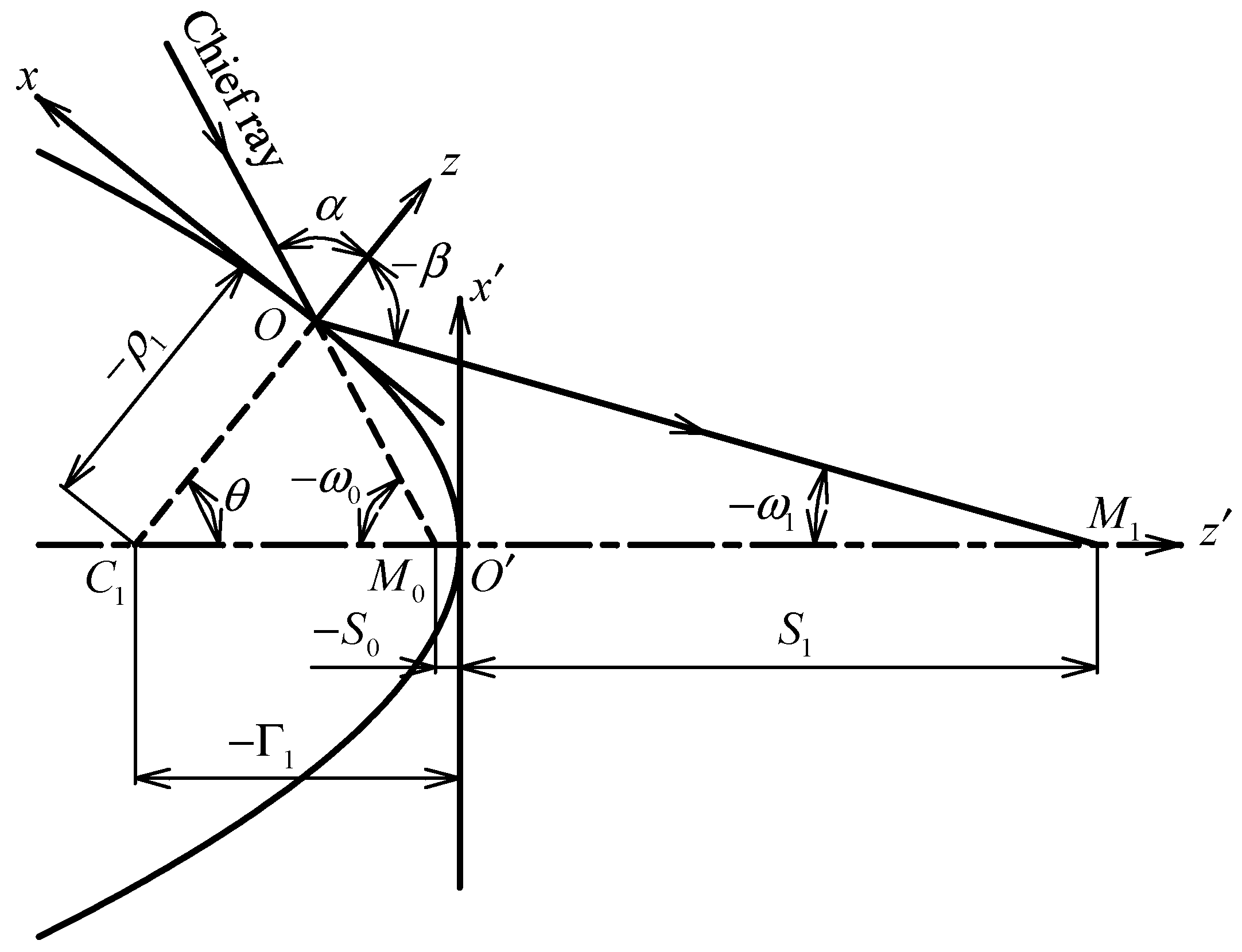
2.1. The Chief Ray Transfer Equation
2.2. Transformation of Figure Equation Coordinate System
3. Calculation Method of the Wave Aberration of a Fisheye Lens
3.1. Aperture Ray Wave Aberrations of an Off-Axis Point Object
3.2. Chief Ray Wave Aberration of an Off-Axis Point Object
4. Determining the Position of Aspheric Surfaces and Aspheric Coefficients
4.1. Evaluation Function
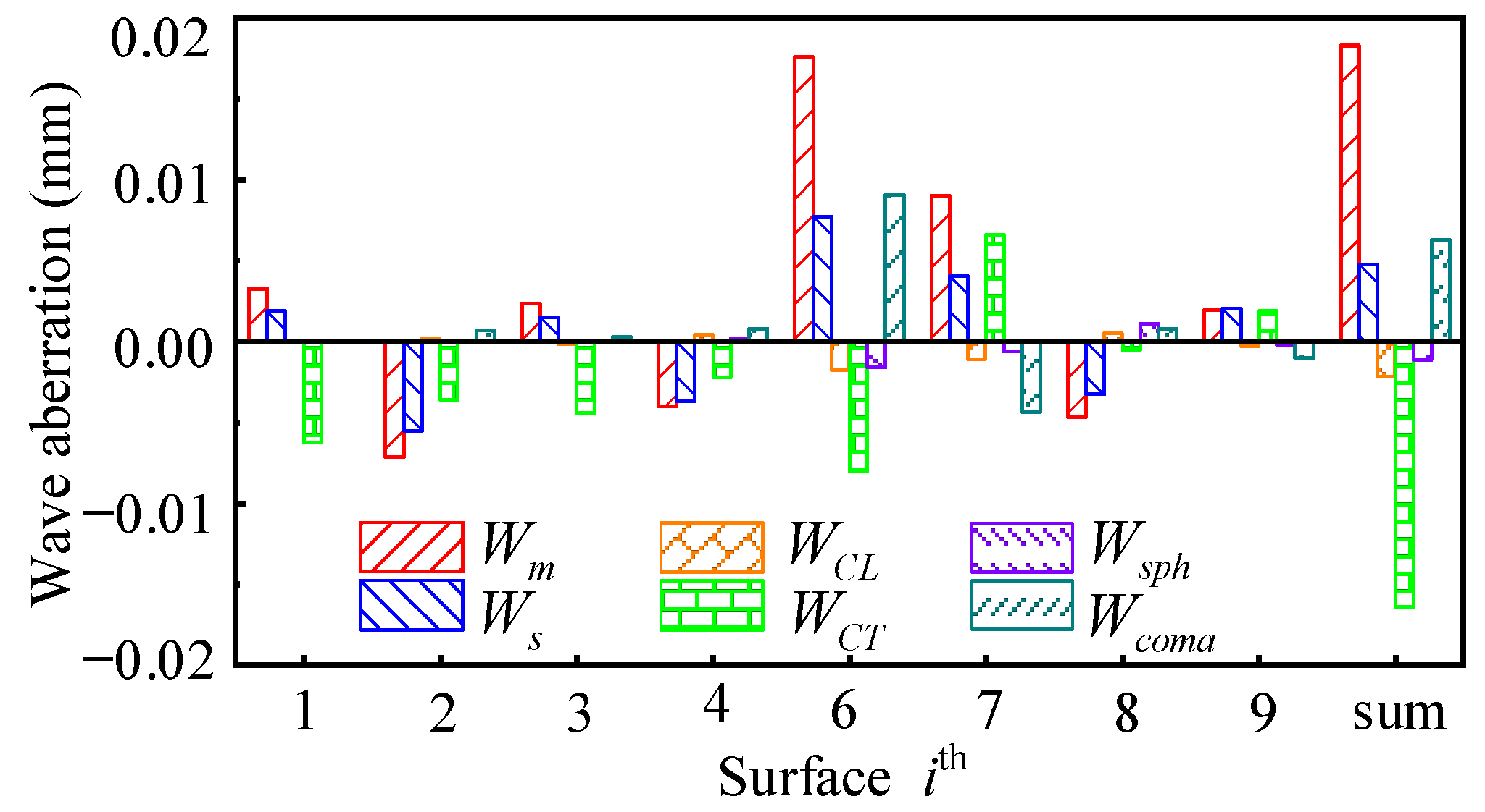
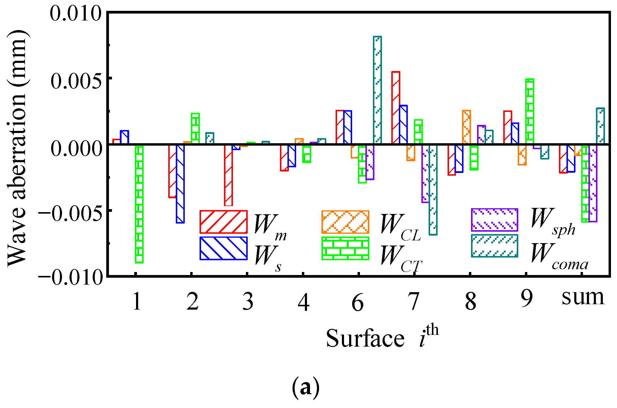
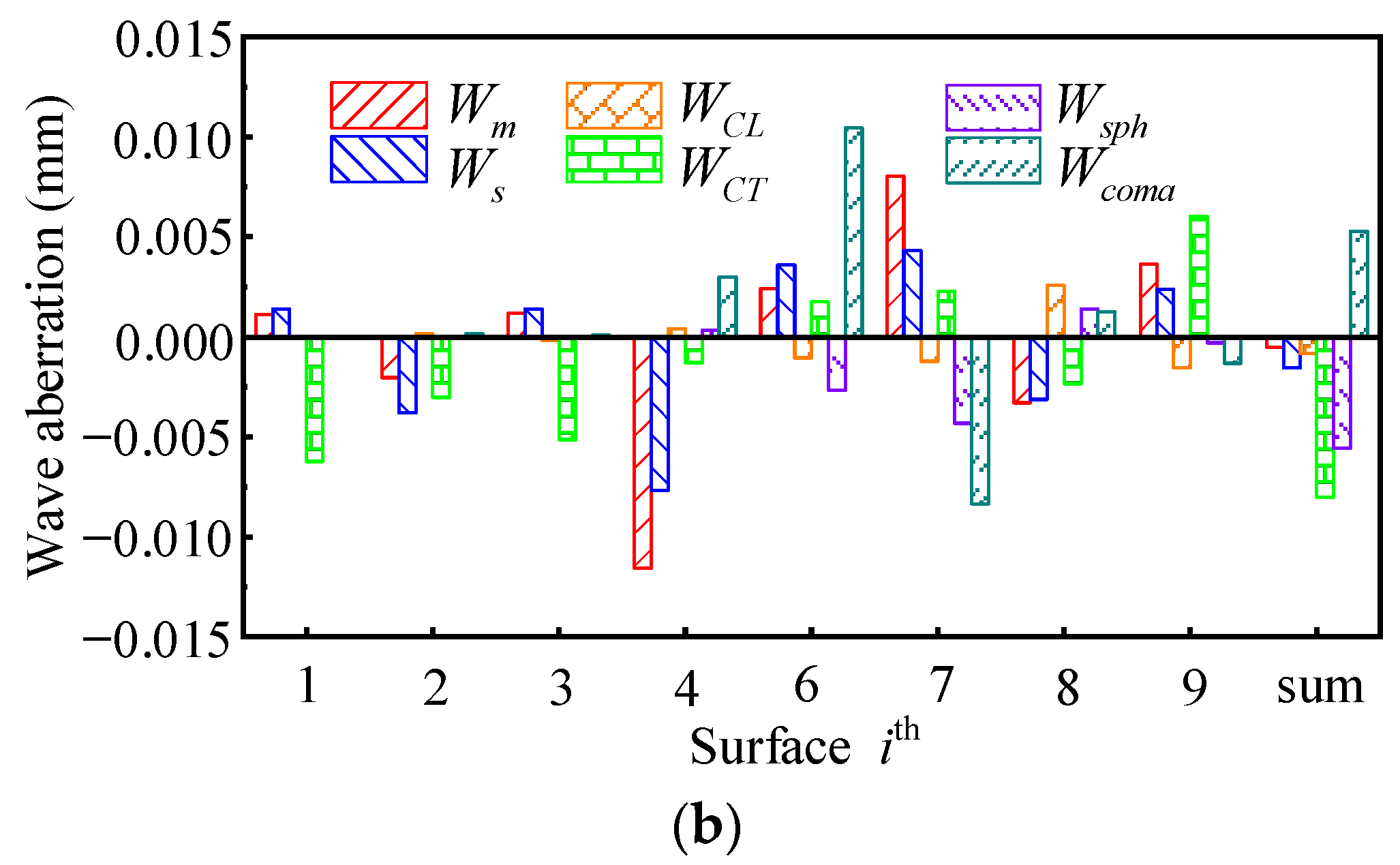
4.2. Wave Aberration Distribution of the Optical Lens
5. Numerical Validation
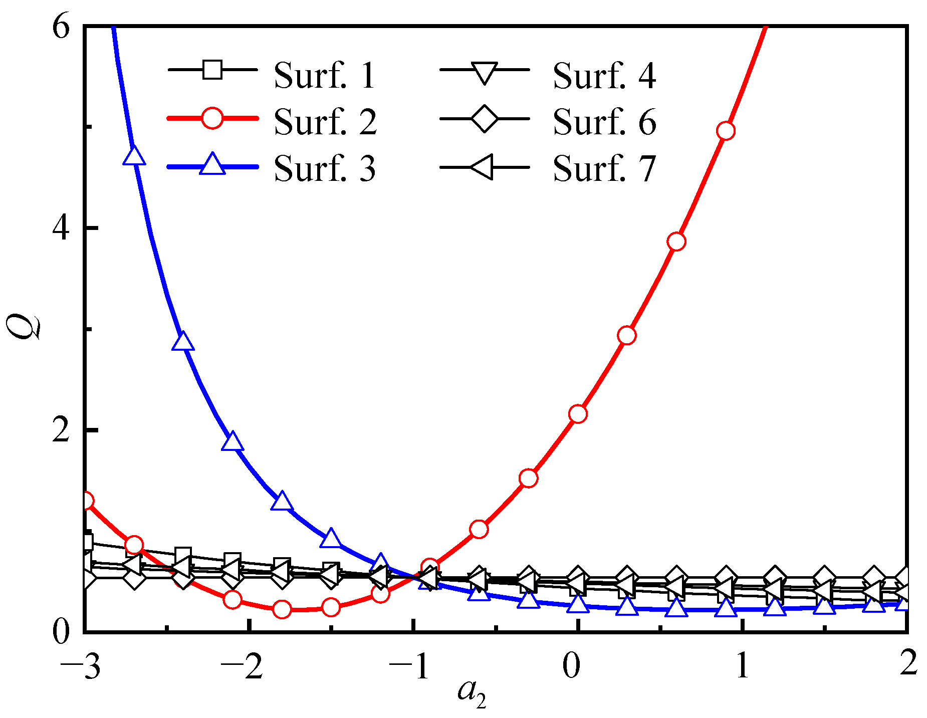
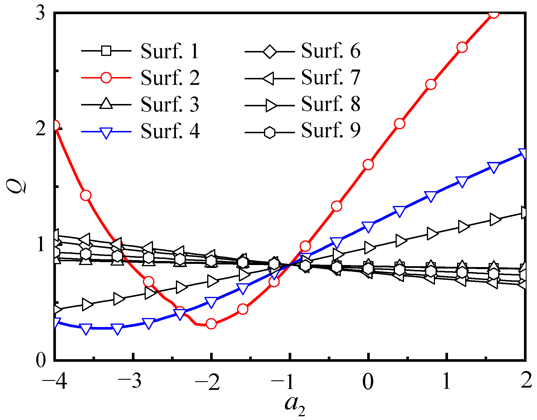
5.1. Determining the Position and Initial Value of Aspheric Surface in the Fisheye Lens
5.2. Optimizing Fisheye Lens III Using an Aspheric Surface
6. Conclusions
- (1)
- In fisheye lenses, the optical surface with a small curvature radius generally adopts an aspheric surface, which is more advantageous for improving its imaging performance. The aspheric coefficient is also closer to the spherical surface, making it easy to manufacture.
- (2)
- In the case of a moderate acceptance aperture of fisheye lenses, the contribution of the aspheric surface to the balance of field curvature aberration is more significant.
Author Contributions
Funding
Institutional Review Board Statement
Informed Consent Statement
Data Availability Statement
Conflicts of Interest
References
- Shannon, R.R. The Art and Science of Optical Design; Cambridge University Press: Cambridge, UK, 1997. [Google Scholar]
- Li, X.; Cen, Z.; Optics, G. Aberrations and Optical Design; Zhejiang University: Hangzhou, China, 2014. [Google Scholar]
- Yabe, A. Optimal selection of aspheric surfaces in optical design. Opt. Express 2005, 13, 7233–7242. [Google Scholar] [CrossRef] [PubMed]
- Yabe, A. Global Optimization with Traveling Aspheric-Aspheric Surface Number as Continuous Variable. In Proceedings of the International Optical Design Conference and Optical Fabrication and Testing, OSA Technical Digest (CD), Jackson Hole, WY, USA, 13–17 June 2010; Optical Society of America: Washington, DC, USA, 2010. [Google Scholar]
- Feng, Y.; Cheng, H.; Wang, T.; Dong, Z.; Tam, H. Optimal strategy for fabrication of large aperture aspheric surfaces. Appl. Opt. 2014, 53, 147–155. [Google Scholar] [CrossRef] [PubMed]
- Zhu, W.; Duan, F.; Tatsumi, K.; Beaucamp, A. Monolithic topological honeycomb lens for achromatic focusing and imaging. Optica 2022, 9, 100–107. [Google Scholar] [CrossRef]
- Pan, J. Design, Manufacture and Test of the Aspherical Optical Surfaces; Suzhou University: Suzhou, China, 2004. [Google Scholar]
- Jing, H.; Wang, S.; Yan, L.; Yan, L.; Shi, C.; Cha, J. Manufacturing of an aluminum alloy off-axis parabolic mirror. Def. Manuf. Technol. 2019, 4, 31–35. [Google Scholar]
- Fan, L.; Lu, L. Calculation of the wave aberration of field curvature and color aberrations of an ultrawide-angle optical system. Optics Commun. 2021, 479, 126414. [Google Scholar] [CrossRef]
- Lu, L. Aberration theory of plane-symmetric grating systems. J. Synchrotron Radiat. 2008, 15, 399–410. [Google Scholar] [CrossRef] [PubMed]
- Chrisp, M.P. Aberrations of holographic toroidal grating systems. Appl. Opt. 1983, 22, 1508–1518. [Google Scholar] [CrossRef]
- Fan, L.; Lu, L. Design of a simple fisheye lens. Appl. Opt. 2019, 58, 5311–5319. [Google Scholar] [CrossRef]
- Lu, L.-J.; Hu, X.-Y.; Sheng, C.-Y. Optimization method for ultra-wide-angle and panoramic optical systems. Appl. Opt. 2012, 51, 3776–3786. [Google Scholar] [CrossRef] [PubMed]
- Lu, L.; Deng, Z. Geometric characteristics of aberrations of plane-symmetric optical system. Appl. Opt. 2009, 48, 6946–6960. [Google Scholar] [CrossRef] [PubMed]
- Zhang, B.; Li, D.; Zhang, S.; Wang, J. Design of aspheric fisheye lens and study of distortion correction algorithm. Acta Optica Sinica 2014, 34, 222–227. [Google Scholar]
- The Inst. of Optics, Handbook of Lenses, No. 6; (National Defense Technology, 1983).
- Zemax User’s Guide; Zemax Development Corporation: Bellevue, WA, USA, 2007.
- Lin, X. ZEMAX Optical Design Super Learning Manual; Posts and Telecommunications Press: Beijing, China, 2014. [Google Scholar]


| Surface i | Radius/mm | Spacing/mm | Index | Glass |
|---|---|---|---|---|
| Object | Infinite | 2000.0 | ||
| 1 | 35.0 | 5.0 | 1.84666 | N-SF57 |
| 2 | 15.0 | 1.0 | ||
| 3 | 15.0 | 12.0 | 1.45600 | N-FK58 |
| 4 | −25.0 | 5.0 | ||
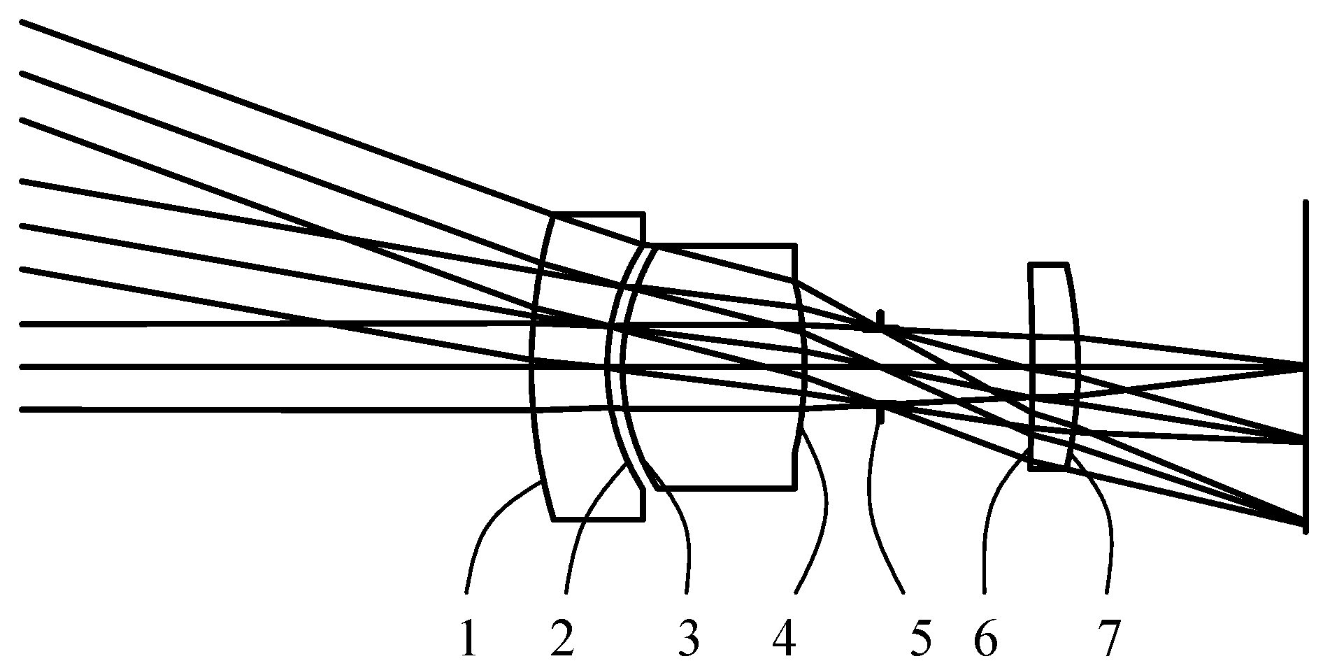
| 5 (STO) | Infinite | 10.0 | ||
| 6 | −130.0 | 3.0 | 1.68893 | P-SF8 |
| 7 | −30.0 | 15.0 |
| Surface i | Radius/mm | Spacing/mm | Index | Glass |
|---|---|---|---|---|
| Object | Infinite | 2000.0 | ||
| 1 | 141.445 | 3.808 | 1.71300 | N-LAK8 |
| 2 | 23.059 | 17.392 | ||
| 3 | 87.889 | 4.099 | 1.71300 | N-LAK8 |
| 4 | 25.685 | 41.513 | ||
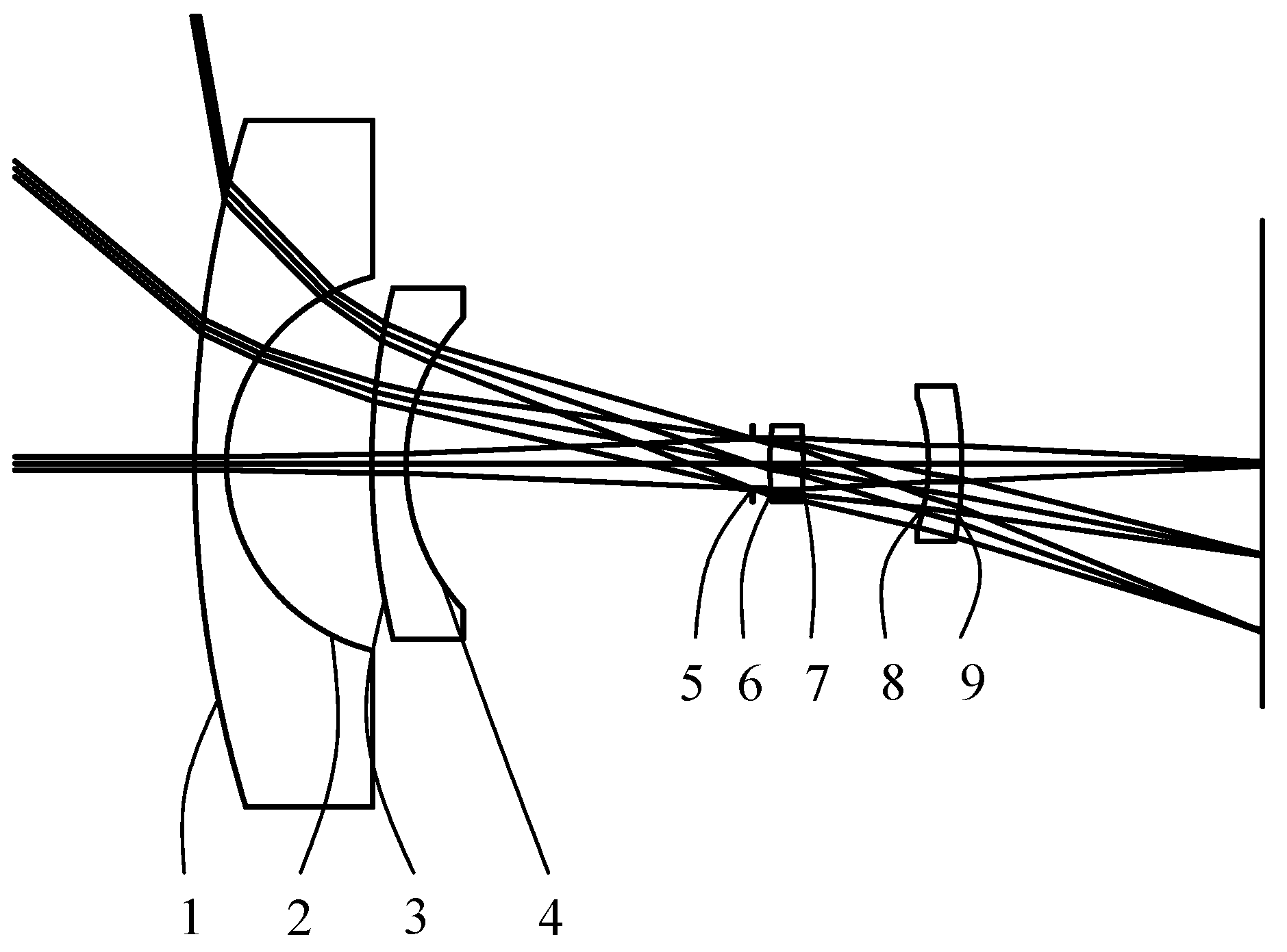
| 5 (STO) | Infinite | 2.0 | ||
| 6 | 30.0 | 4.0 | 1.71300 | N-LAK8 |
| 7 | −80.0 | 15.0 | ||
| 8 | −24.0 | 4.0 | 1.45600 | N-FK58 |
| 9 | −50.0 | 31.101 | - | - |
| Lens I | Fisheye Lens II | |||
|---|---|---|---|---|
| Surface | 2 | 3 | 2 | 4 |
| −1.69 | 0.79 | −2.12 | −3.42 | |
| Surface i | Radius/mm | Spacing/mm | Index | Glass | ||
|---|---|---|---|---|---|---|
| Original | Optimized | Original | Optimized | |||
| 1 | 162.236 | 148.852 | 7.676 | 5.946 | 1.5163 | BK7HT |
| 2 | 69.168 | 35.582 | 28.975 | 29.988 | - | - |
| 3 | 98.314 | 60.443 | 4.186 | 3.716 | 1.6127 | SK4 |
| 4 | 42.474 | 35.560 | 13.054 | 10.810 | - | - |
| 5 | 64.484 | 41.520 | 4.210 | 3.521 | 1.6148 | SSK3 |
| 6 | 12.623 | 13.644 | 13.536 | 13.741 | - | - |
| 7 | −105.027 | −170.440 | 1.297 | 1.219 | 1.4875 | N-FK5 |
| 8 | 18.953 | 14.957 | 4.535 | 5.050 | 1.7847 | SF56A |
| 9 | −232.713 | −273.525 | 1.175 | 1.118 | 1.7555 | P-LAF37 |
| 10 | 75.791 | 74.989 | 13.862 | 12.265 | - | - |
| 11 (STO) | ∞ | ∞ | 2.528 | 2.843 | - | - |
| 12 | 57511.3 | 53039.16 | 1.364 | 1.396 | 1.7847 | SF56A |
| 13 | 15.425 | 13.347 | 8.586 | 7.203 | 1.7433 | N-LAF35 |
| 14 | −46.059 | −63.238 | 0.142 | 0.117 | - | - |
| 15 | −259.655 | −316.890 | 4.751 | 4.043 | 1.7555 | P-LAF37 |
| 16 | −37.371 | −36.438 | 18.493 | 16.484 | - | - |
| 17 | 38.3731 | 34.778 | 2.524 | 2.169 | 1.7847 | SF56A |
| 18 | 24.438 | 19.829 | 19.820 | 23.887 | 1.6204 | N-SK16 |
| 19 | −53.609 | −43.558 | 12.963 | 12.006 | - | - |
| 0 | 10 | 20 | 30 | 40 | 50 | 60 | 70 | 80 | ||
|---|---|---|---|---|---|---|---|---|---|---|
| Frist round | 1 | 1 | 1 | 1 | 2 | 2 | 2 | 2 | 2 | |
| Second round | 1 | 1 | 2 | 2 | 4 | 4 | 6 | 6 | 7 |
Disclaimer/Publisher’s Note: The statements, opinions and data contained in all publications are solely those of the individual author(s) and contributor(s) and not of MDPI and/or the editor(s). MDPI and/or the editor(s) disclaim responsibility for any injury to people or property resulting from any ideas, methods, instructions or products referred to in the content. |
© 2023 by the authors. Licensee MDPI, Basel, Switzerland. This article is an open access article distributed under the terms and conditions of the Creative Commons Attribution (CC BY) license (https://creativecommons.org/licenses/by/4.0/).
Share and Cite
Fan, L.; Yan, K.; Qiao, G.; Lu, L.; Gao, S.; Zheng, H. Determination Position and Initial Value of Aspheric Surface for Fisheye Lens Design. Photonics 2023, 10, 1381. https://doi.org/10.3390/photonics10121381
Fan L, Yan K, Qiao G, Lu L, Gao S, Zheng H. Determination Position and Initial Value of Aspheric Surface for Fisheye Lens Design. Photonics. 2023; 10(12):1381. https://doi.org/10.3390/photonics10121381
Chicago/Turabian StyleFan, Lirong, Ketao Yan, Guodong Qiao, Lijun Lu, Shuyuan Gao, and Huadong Zheng. 2023. "Determination Position and Initial Value of Aspheric Surface for Fisheye Lens Design" Photonics 10, no. 12: 1381. https://doi.org/10.3390/photonics10121381
APA StyleFan, L., Yan, K., Qiao, G., Lu, L., Gao, S., & Zheng, H. (2023). Determination Position and Initial Value of Aspheric Surface for Fisheye Lens Design. Photonics, 10(12), 1381. https://doi.org/10.3390/photonics10121381