1. Introduction
After the discovery of graphene by A. Geim and K. Novoselov [
1], the so-called two-dimensional materials, which are considered infinitely thin in a mathematical model and are modeled using special conditions on the surface of a substrate, began to be actively studied. Graphene is the most popular and promising two-dimensional material due to a number of unique properties. It is a layer that is one atom thick and forms a hexagonal crystal lattice of carbon atoms. Graphene is already being used in photonics and optoelectronics. In addition, graphene can also be used in waveguide structures to improve their characteristics. In particular, graphene can be used in various optical devices, such as photodetectors, modulators, and polarizers [
2].
A large number of papers have been published on the propagation of electromagnetic waves in waveguide devices containing graphene. Most often, TE and TM waves propagating in a dielectric layer coated with graphene are studied [
3,
4,
5]. Moreover, graphene can be located on both sides of the dielectric layer and is able to support plasmon modes [
6,
7,
8]. Plane structures consisting of several alternating layers of dielectric and graphene have also been considered [
9].
Graphene nonlinearity was predicted in [
10,
11], and, later, in [
12], it received experimental confirmation. A third-order nonlinearity was found in the terahertz and infrared frequency ranges, similar to the well-known Kerr’s law. Attempts have been made to use the effect of graphene nonlinearity in photonic devices [
13].
This article is devoted to the development of a numerical method for determining the propagation constants of surface, complex, and leaky modes of monochromatic TE-polarized waves in an inhomogeneous Goubau line coated on one side with graphene. At the same time, we take into account the nonlinearity of graphene, which is expressed in changing the standard interface conditions at the interface of media to special conditions containing a nonlinear dependence of conductivity on the intensity of the surface electric field.
Such a statement of the boundary value problem for the system of Maxwell’s equations leads to the need to develop new numerical methods for solving the problem, since nonlinear problems of this type have not been studied before. In our formulation of the problem, there are a number of restrictions on the parameters of the waveguide structure. First of all, we do not take into account the absorption in either the dielectric layer or graphene. This assumption is often implemented in practice, since the absorption in the terahertz range is small compared to the strong plasmon response of graphene. In addition, we assume that the conductivity of the graphene depends only on the tangential components of the electric field, more precisely, on its intensity. In this case, the nonlinear part of the conductivity is determined by the amplitude of the TE wave and does not depend on the longitudinal coordinate. This allows us to consider arbitrary, including complex, constant propagations and to study not only surface modes but also complex and leaky modes as well. At the same time, graphene nonlinearity is taken into account in all cases.
From a mathematical point of view, we deal with eigenvalue problems for one differential equation in the case of TE waves with “non-classical” boundary conditions: on the inner boundary, we have one homogeneous condition of the first kind and an additional nonhomogeneous condition of the second kind, which is required in order to determine a discrete set of solutions, and on the external boundary, we have a condition that is nonlinear with respect to a sought-for function.
We will obtain a dispersion equation with the property that its solution is an eigenvalue of the corresponding problem and, conversely, any eigenvalue of the problem is a solution to the dispersion equation. By studying characteristic equations, we will obtain sufficient conditions ensuring that the considered eigenvalue problem has solutions. From a physical point of view, this means that if these conditions are satisfied, then the waveguiding structure studied in the paper is able to support TE-eigenwaves.
An analysis of wave propagation in open metal–dielectric waveguides constitutes an important class of electromagnetic problems. A conducting cylinder covered by a concentric dielectric layer, the Goubau line, is the simplest type of such guiding structures. A complete mathematical investigation of the spectrum of symmetric surface modes in a Goubau line is performed in [
14,
15,
16].
A large number of papers have been devoted to the study of electromagnetic properties of structures containing graphene layers. Many properties of such structures have been studied quite fully, and there is a significant number of their applications in practice (see, for example, [
17,
18,
19,
20,
21,
22]).
The classification of waves existing in the Goubau line is an urgent task in the study of waveguides. In this work, a general formulation of the problem is proposed, covering a wide class of TE-polarized waves and various materials filling the waveguide. A numerical method that allows one to calculate the wave propagation constants is proposed. The numerical method is based on the solution to an auxiliary Cauchy problem. Based on this method, it is possible to classify electromagnetic TE-polarized waves existing in a Goubau line: leaky and surface waves (depending on the condition at infinity) and evanescent, propagating and complex waves (depending on the propagation constant).
In this paper, the problem of the propagation of a TE wave in a Goubau line coated with graphene is considered. The graphene coating is considered infinitely thin and leads to a change in one conjugation condition when setting the problem. Such a model is determined by the fact that the graphene layer has a thickness of the order of one atom. Since graphene exhibits nonlinearity, in this article, we will take nonlinearity into account.
The article presents the calculations of the Goubau line filled with a dielectric, inhomogeneous dielectric, dielectric with losses and metamaterial. The calculations were made at different frequencies. Thus, we numerically found complex, evanescent, and propagating leaky waves and complex, evanescent, and propagating surface waves.
2. Statement of the Problem
Consider the three-dimensional space
equipped with the cylindrical coordinate system
and filled with a isotropic source-free medium with permittivity
and permeability
, where
and
are the permittivity and permeability of a vacuum. We consider electromagnetic waves propagating through a Goubau line:
and a generating line parallel to the axis
is placed in
.
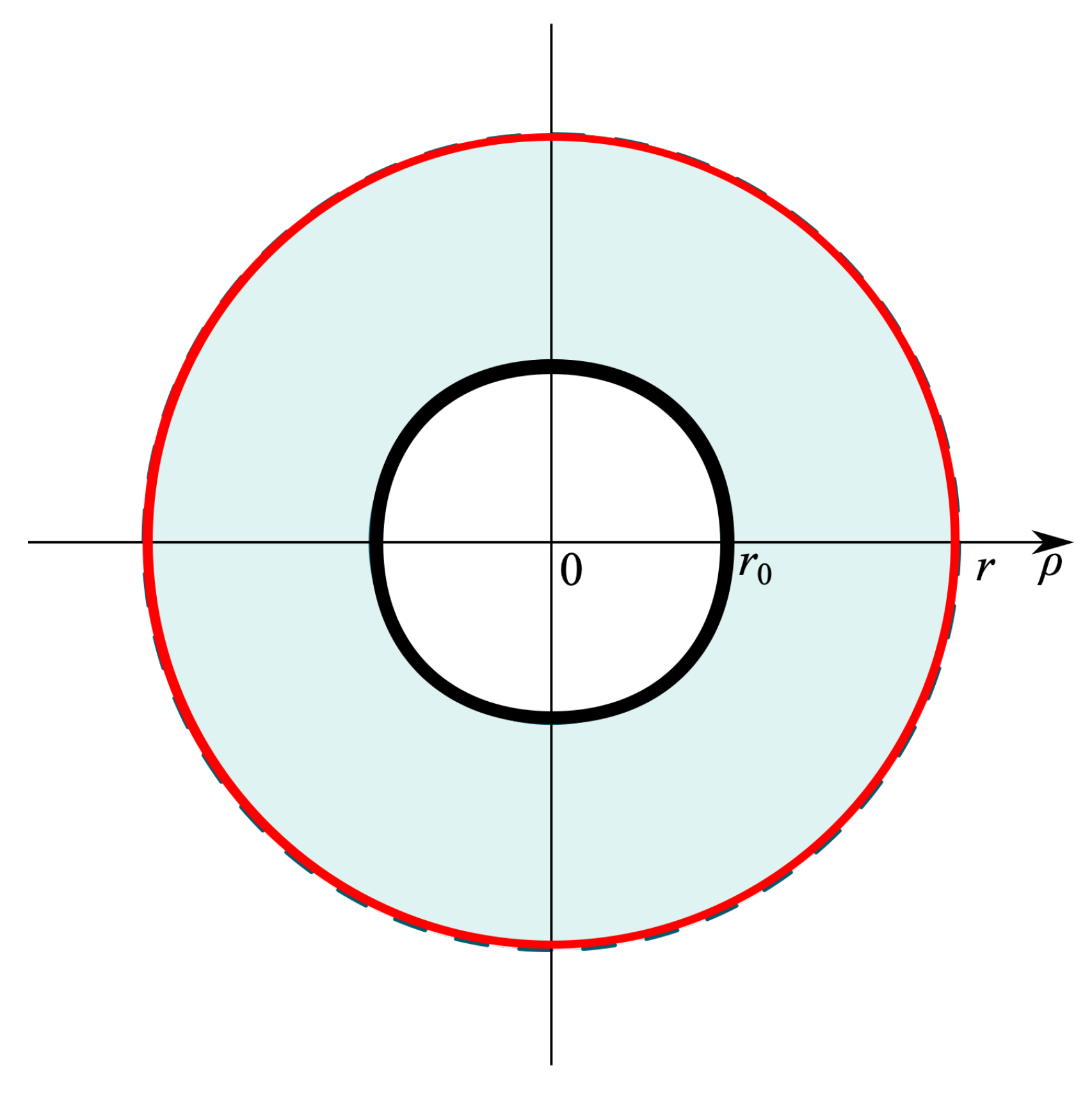
The cross section of the Goubau line consists of two concentric circles with radii
and
r (see
Figure 1):
is the radius of the internal (perfectly conducting) cylinder, and
is the thickness of the external cylindrical shell.
We assume that the fields depend harmonically on time as , where is the circular frequency.
The determination of TE-polarized waves reduces to finding nontrivial running-wave solutions of the homogeneous system of Maxwell equations depending on the coordinate
z along which the structure is regular in the form
,
with boundary conditions for a tangential electric field component on a perfectly conducting screen
and the transmission conditions for the tangential electric and magnetic field components on the permittivity discontinuity surface (
)
where
and
and
.
We will not fix the radiation condition at infinity because we want to consider the problem for arbitrary .
We assume that the relative permittivity in the entire space has the form
We also assume that
is a continuous function on the segment
, i.e.,
.
The problem of normal waves is an eigenvalue problem for the Maxwell equations with spectral parameter , which is the propagation constant of waveguiding structure.
The normal wave field in the waveguide can be represented using one scalar function
Thus, the problem is reduced to finding the tangential component of the electric field
u. Throughout the text below,
stands for differentiation with respect to
.
Definition 1. The propagating wave is characterized by the real parameter γ.
Definition 2. The evanescent wave is characterized by the pure imaginary parameter γ.
Definition 3. The complex wave is characterized by the complex parameter γ such that .
Definition 4. The surface wave satisfies the condition , .
Definition 5. The leaky wave satisfies the condition , .
Remark 1. The Propagation constant γ characterises the behavior of a wave (propagating, evanescent, or complex) in the z direction. The classification of waves as surface or leaky depends on the behavior in the ρ-direction.
We have the following eigenvalue problem for the tangential electric field component
u: find
such that there exist nontrivial solutions of the differential equation
satisfying the boundary conditions
and the transmission conditions
where
Thus the resulting field
will satisfy all conditions (
1)–(
3).
For
, we have
; then, from (
4), we obtain the equation
In accordance with the condition at infinity (see Definitions 4 and 5), we choose a solution to the last equation for surface waves in the form
and for leaky waves
where
and
,
and
are the constants, and
and
are the modified Bessel functions (Macdonald and Infeld functions) [
23].
For
, we have
; thus, from (
4), we obtain the equation
where
Definition 6. is called a propagation constant of the problem if there exists a nontrivial solution u to Equation (10) for , satisfying, for , solutions (8) for surface waves and (9) for leaky waves, respectively, the boundary condition (5), and the transmission conditions (6). 3. Numerical Method
Let us consider the Cauchy problem for Equation (
10) with the initial conditions
where
A is a known constant.
We assume that the Cauchy problem (
10), (
12) is globally and uniquely solvable on the segment
for given values
,
r, and its solution continuously depends on the parameter
. Using the transmission condition on the boundary
(
6), one has the dispersion equation for surface waves
and the dispersion equation for leaky waves
where quantities
and
are obtained from the solution to the Cauchy problem (
10), (
12).
Let
where
. Then, equating to zero the real and imaginary parts of
, one obtains a system of real equations for determining the real and imaginary parts of the complex parameter
:
We will numerically solve a system of Equation (
15) to determine the pair
. The solution to each equation of the system (
15) is a curve in the plane
. Then, we determine points of intersections of the curves; these points are approximate eigenvalues of the problem. Let us introduce a grid
with a step
in
and a step
in
, where
,
,
,
are real fixed constants. We use grid points for the shooting method.
Solving the Cauchy problem (
10), (
12) for each grid point, one obtains
and
,
,
. Since the solution
is continuously dependent on the parameters
and
, it follows that there exists a point
in the plane
where
, such that
The less
and
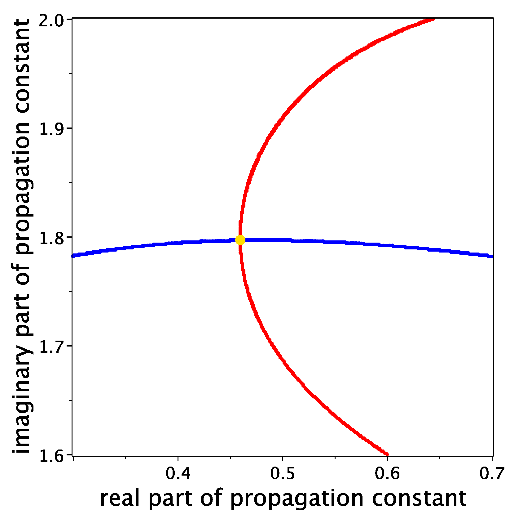
, the more exact a solution. Continuing in the same way, one finds a set of pairs
that are a curve in the plane
(the blue curve in
Figure 2).
Applying the same approach to the second equation of (
15), one obtains another curve in the plane
(the red curve in
Figure 2). This curve is an approximate solution to the equation
. It is clear that the intersection points of the curves (the yellow point in
Figure 2) are approximate solutions of the problem. By decreasing the steps
and
, we can obtain arbitrarily accurate solutions.
4. Numerical Results
In
Figure 3,
Figure 4,
Figure 5,
Figure 6,
Figure 7,
Figure 8,
Figure 9 and
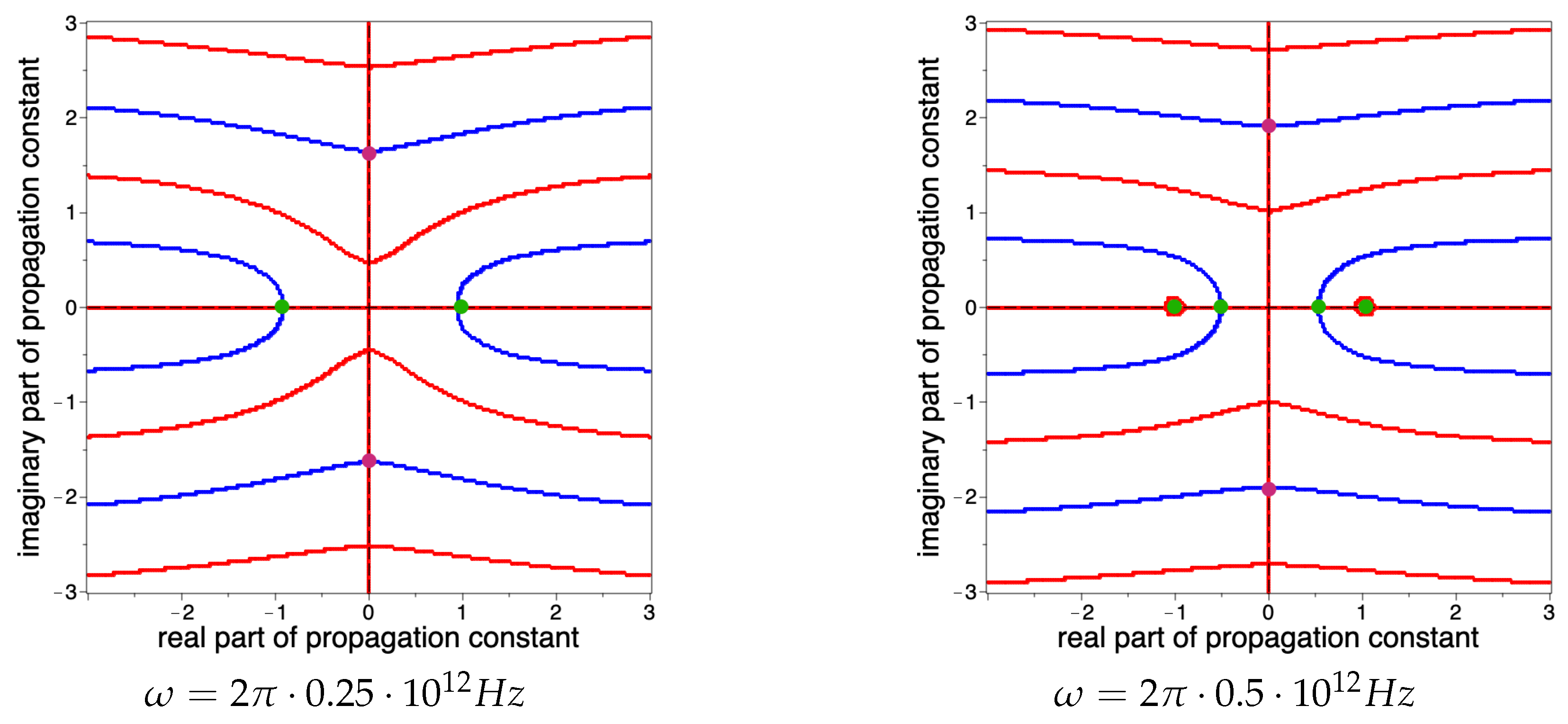
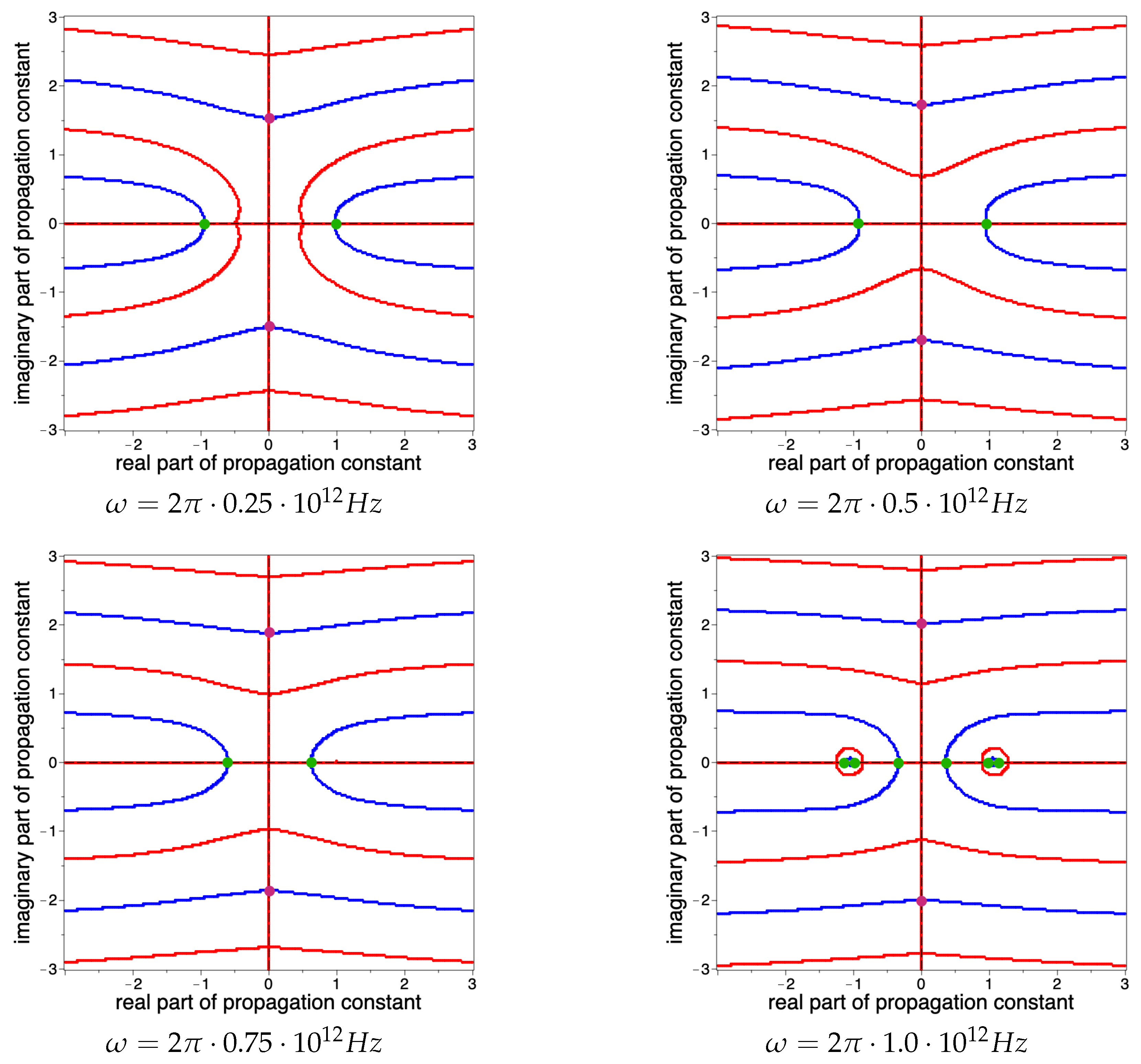
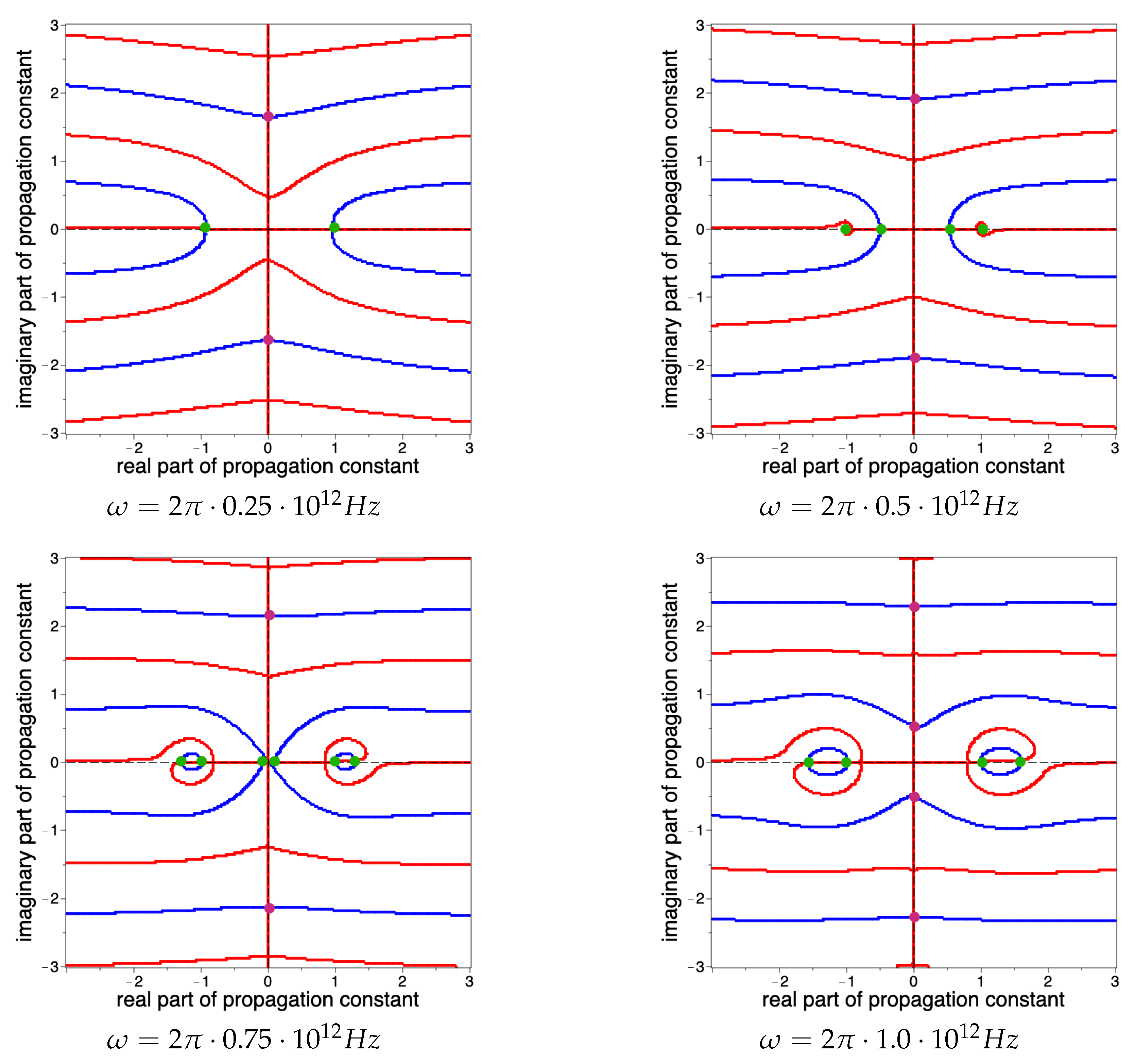
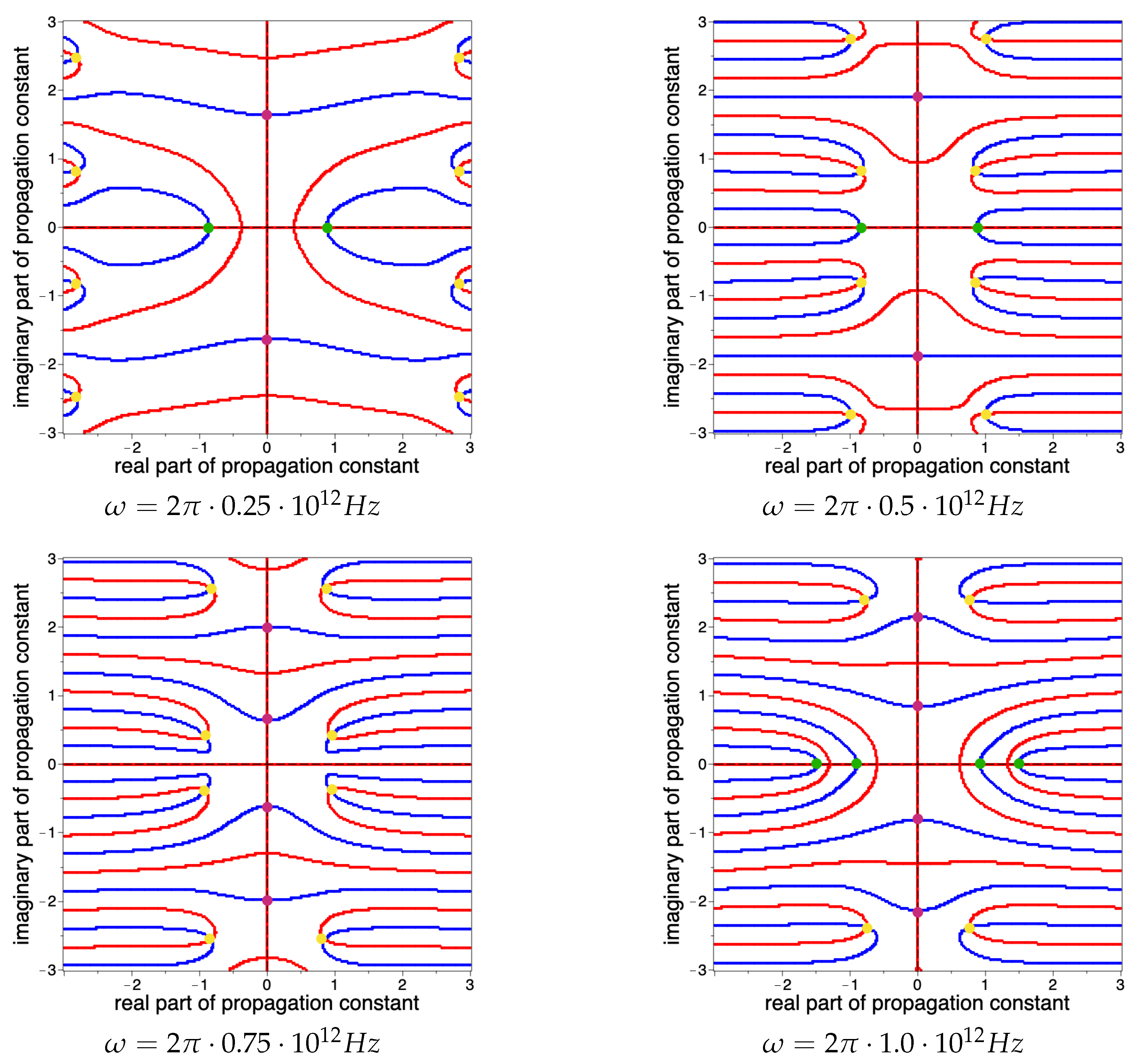
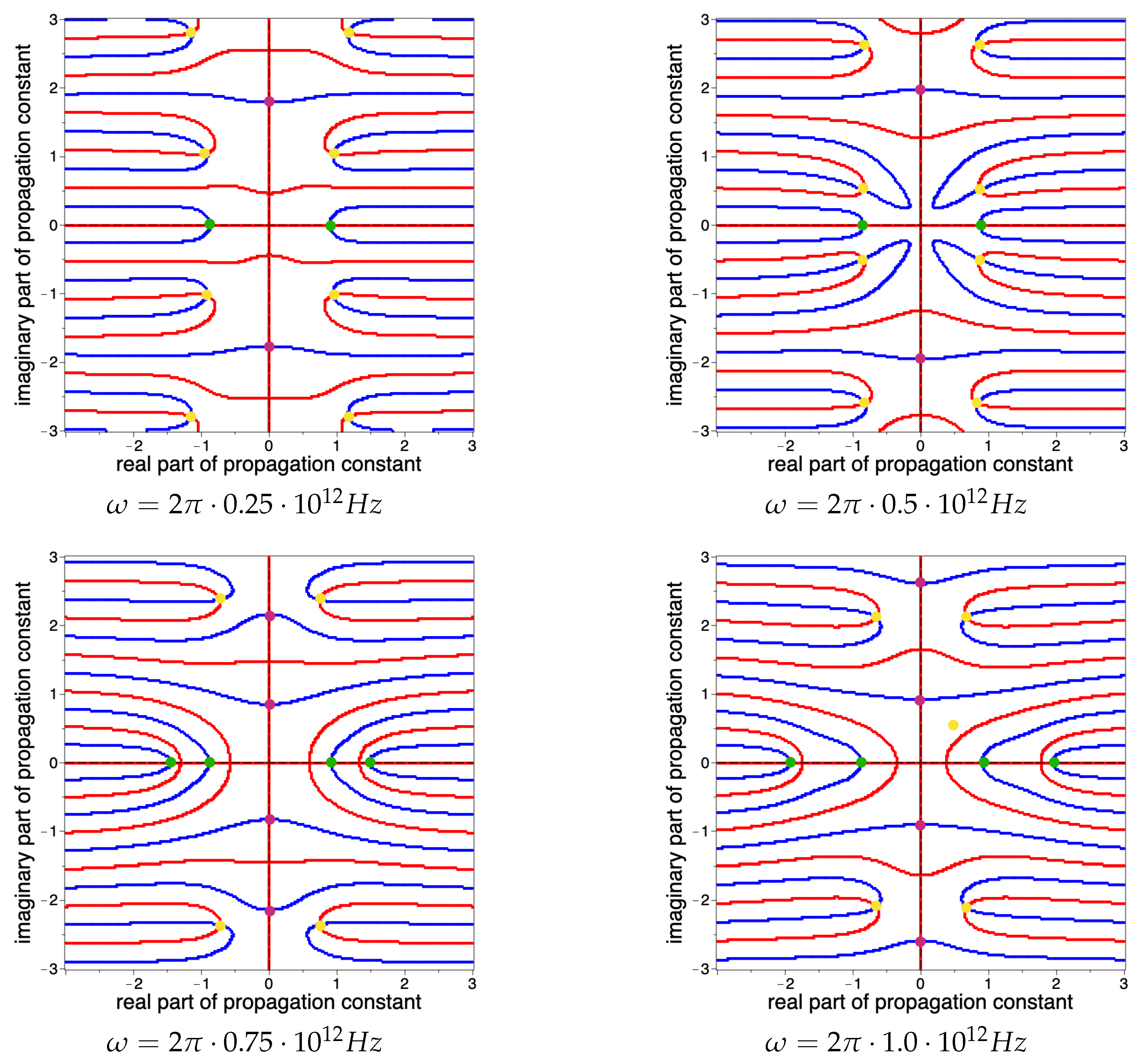
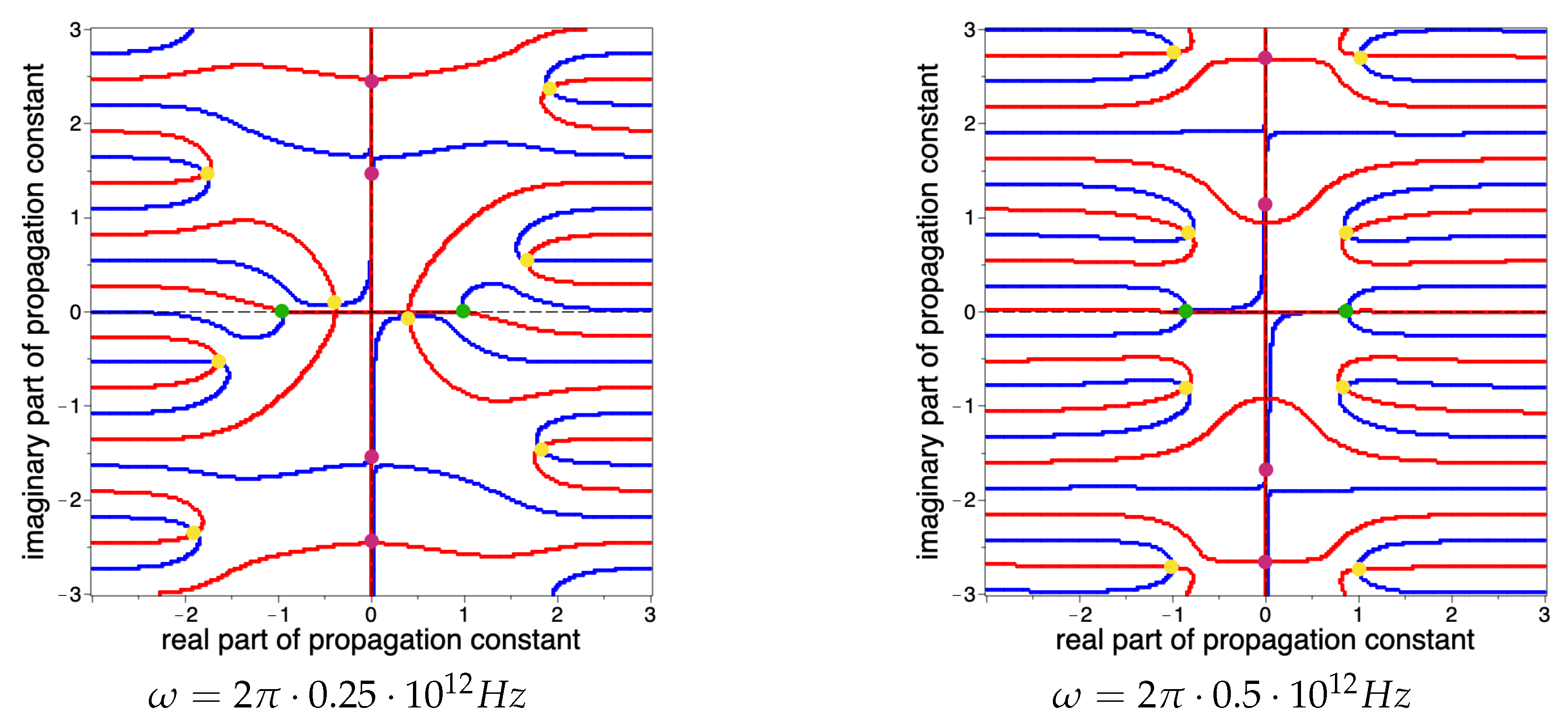
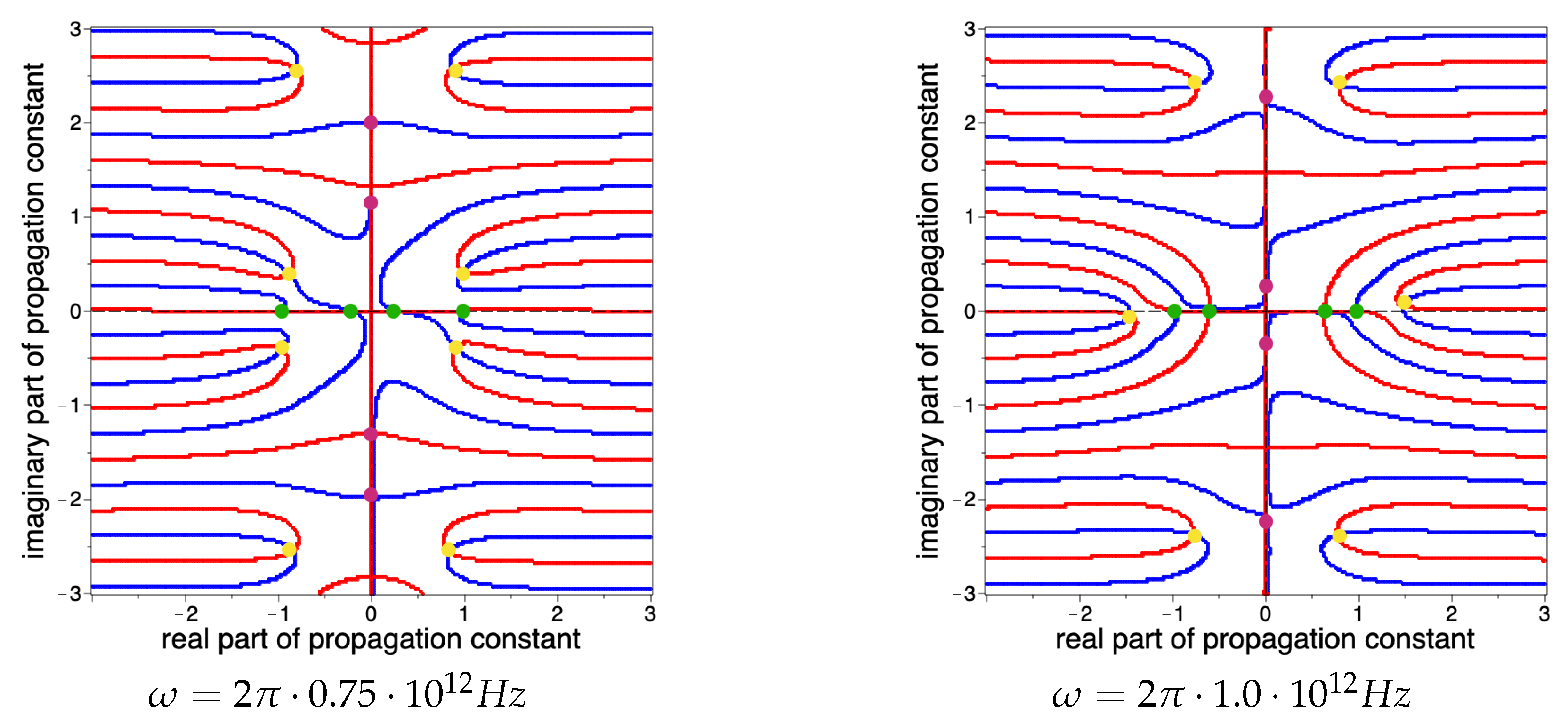
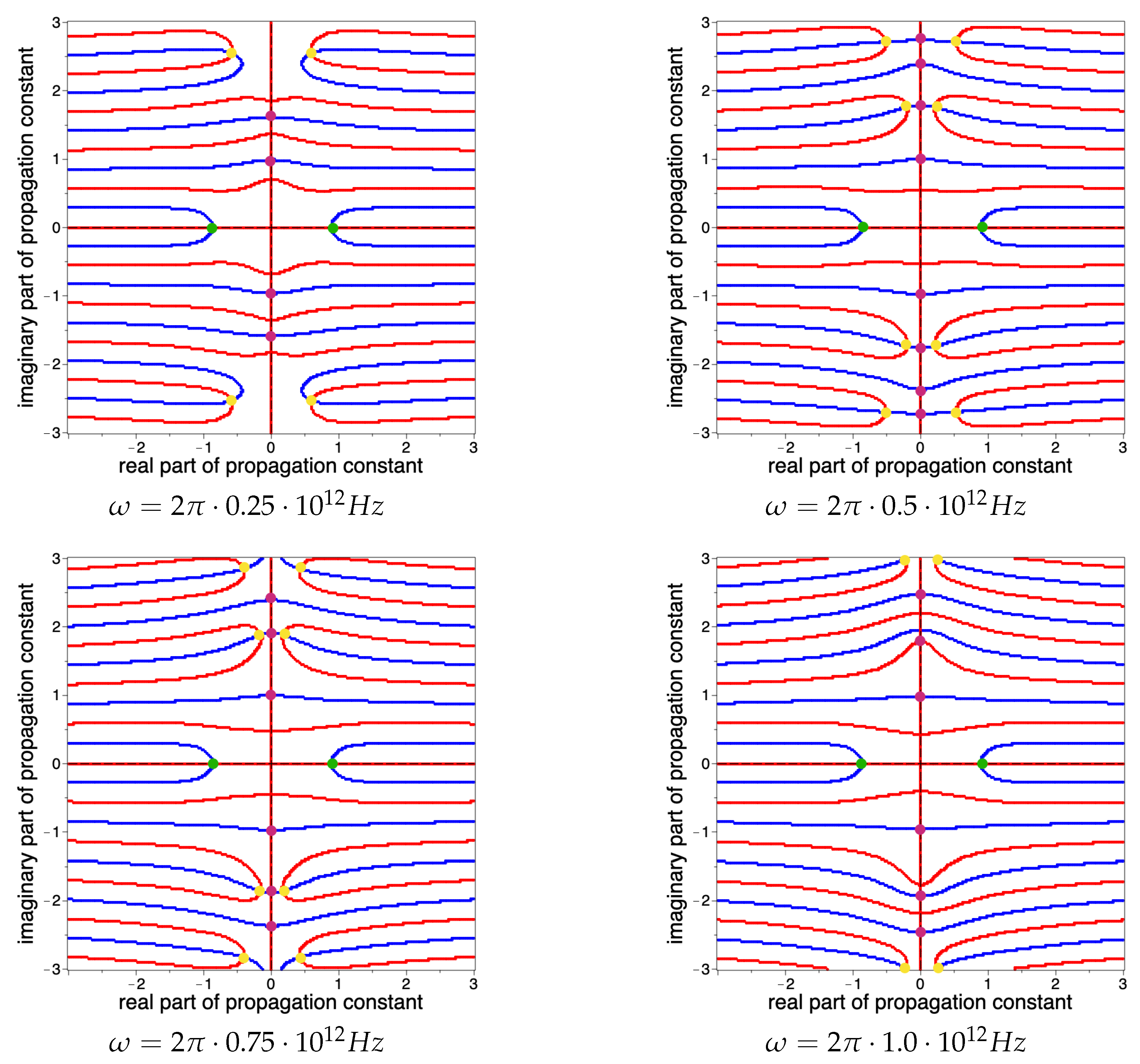
Figure 10, the results of calculating the propagation constants for the problem of the propagation of TE-polarized waves in a Goubau line filled with a dielectric, inhomogeneous dielectric, dielectric with losses, and metamaterial are presented. We have carried out numerical experiments for four frequency values. Propagating, evanescent, complex surface TE waves, and propagating, evanescent, and complex leaky TE waves are found.
The following values of parameters are used for calculations: S · m2· V−2, S · m2 · V−2, , , , V · m−1, m, m, , , , , , .
In
Figure 3,
Figure 4,
Figure 5 and
Figure 6, the solutions to the problem of surface TE waves in a Goubau line are presented. There are no complex surface TE waves (yellow points). In
Figure 3 and
Figure 6, we have carried out numerical experiments for a dielectric with constant permittivity and a dielectric with losses. In these cases, propagating surface TE waves (green points) do not exist at all frequencies. If the waveguide is filled with an inhomogeneous dielectric (as in
Figure 4), then with increasing frequency, the number of propagating surface TE waves increases; in addition, values of real propagating constants increase in the modulus. In the case of a metamaterial (see
Figure 6), with increasing frequency, the absolute values of the propagation constants corresponding to the evanescent surface TE waves decrease, and the absolute values of the propagation constants corresponding to the propagating surface TE waves increase.
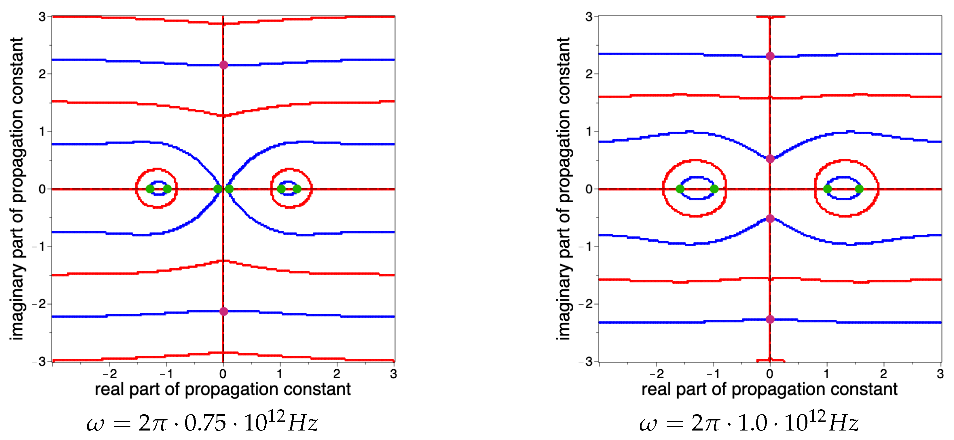
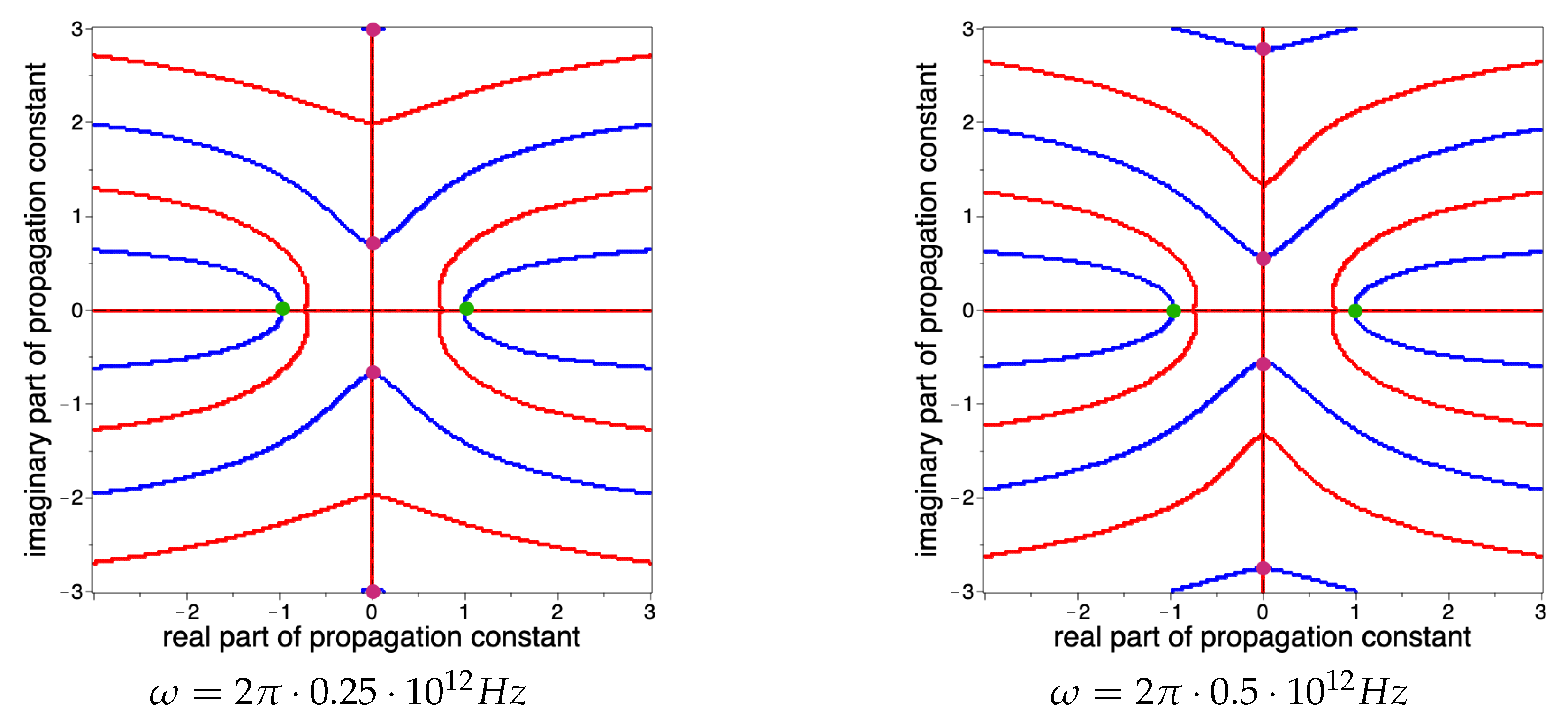
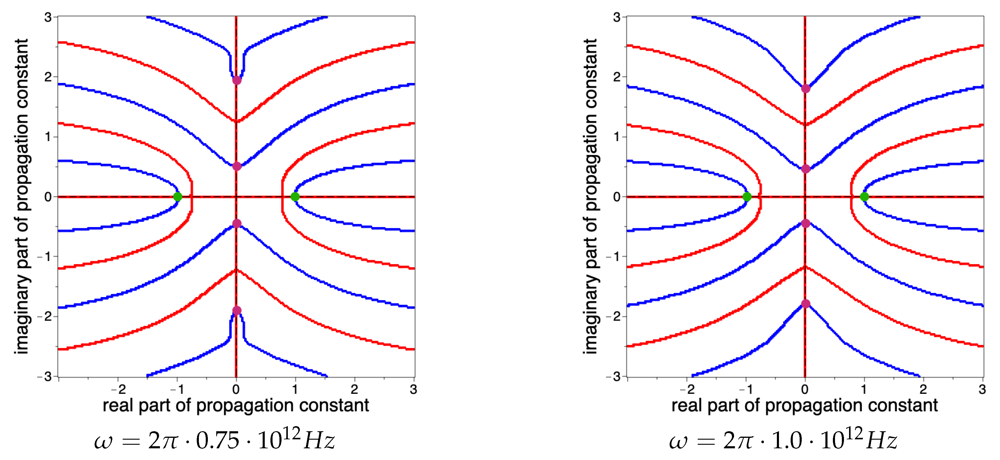
In
Figure 7,
Figure 8,
Figure 9 and
Figure 10, solutions to the problem of leaky TE waves in a Goubau line are shown. In the case of a homogeneous dielectric with constant permittivity, all types of leaky TE waves exist at all chosen frequencies (see
Figure 7). It can be seen, that with increasing frequency, the absolute values of the real propagation constants increase, the absolute values of the complex propagation constants decrease, and the number of the imaginary propagation constants increases. This trend continues in the case of homogeneous dielectric shown in
Figure 8 and in the case of dielectric with losses shown in
Figure 9. In the case of a metamaterial (see
Figure 10), propagating leaky TE waves (green points) do not exist at all frequencies. In the case with increasing frequency, the absolute values of the imaginary part of the propagation constants corresponding to the complex surface TE waves (yellow points) increase, and the absolute values of the real part of the propagation constants tend to zero.
5. Conclusions
We have developed a numerical method of analysis of the surface TE wave propagation in an inhomogeneous metal–dielectric waveguide structure coated with graphene. The physical problem is reduced to a transmission eigenvalue problem for Maxwell’s equations. Using the solutions to an auxiliary Cauchy problem with initial conditions on the boundary and transmission conditions on the boundary , it is possible to obtain the dispersion equations for surface and leaky waves. The numerical determination of approximate solutions is performed using a version of the shooting method developed specifically for this class of problems.
It can be seen from the numerical results that propagating surface waves and propagating leaky waves exist only at certain frequencies. In addition, complex surface waves were not found.
6. Discussion
In this paper, the problem of propagation of an electromagnetic TE wave in an inhomogeneous Goubau line with a graphene layer was studied. More precisely, a circular concentric dielectric layer is covered with an infinitely thin layer of graphene. Unlike most similar works, graphene’s nonlinearity is taken into account here, which appears in the terahertz and infrared frequency ranges. In this case, the nonlinearity is described using the Kerr-type law, that is, cubic nonlinearity is considered. Since the graphene layer has a thickness of the order of one atom, only tangential components of the electric field are taken into account in the nonlinearity. In addition, we assume that the nonlinearity is determined only by the amplitudes of the propagating waves and does not depend on the longitudinal coordinate.
We consider both homogeneous and inhomogeneous Goubau lines. Both surface and leaky waves are studied. In all cases, we obtain an implicit dispersion equation by applying a numerical method. With the help of the dispersion equation, the propagation constants corresponding to the eigenwave of the waveguide are determined. Note that the proposed method makes it possible to find not only real but also complex constants of the propagation of normal waves in the Goubau line.
It makes sense to take into account nonlinear effects in graphene when nonlinearity has a significant impact on the propagation of electromagnetic waves, that is, if the radiation is strong enough.
In [
24], the similar nonlinear eigenvalue problem of electromagnetic wave propagation in a plane dielectric layer covered with graphene was considered. In that paper, the dispersion equation was obtained explicitly. Eigenwaves, as well as propagating constants of surface waves, were calculated. In this paper, we consider not only surface waves but also leaky and complex waves.
Note that we did not obtain an explicit dispersion equation. Our approach is very different. First, we reduce the boundary eigenvalue problem to a Cauchy problem using initial conditions. Then, we solve the Cauchy problem numerically via an appropriate code. Thus, we obtain dispersion equations at the external boundary. The dispersion equation is solved with respect to a spectral parameter, i.e., the propagating constant.
Usually, along with TE-polarized waves, TM-polarized waves in the waveguide structure are also considered. In this article, we have focused on the study of only TE-polarized waves, but TM waves can also be studied using the proposed method. But when studying TM waves, it is already necessary to change the formulation of the problem, so it is natural to consider this case separately. The case of hybrid waves is interesting when both electric and magnetic longitudinal components of an electromagnetic wave take place. In this case, the proposed research method is also applicable, but the system of differential equations becomes much more complicated.
In addition to the waveguide structure discussed in this article, it is interesting to study more complex configurations consisting of several dielectric concentric layers with graphene coatings on each of them. It is not difficult to see that the method will again be applicable to finding the propagation constants of surface, complex, and leaky waves. Such structures can be very useful in practice. It should also be noted that the problem investigated in the article is new from a mathematical point of view since nonlinear coupling conditions are very exotic in mathematical physics and, as far as the authors know, have not been considered before. Therefore, the development of new numerical methods for solving nonlinear eigenvalue problems of this type is an urgent problem in mathematical physics.


