A Laser Triangulation Displacement Sensor Based on a Cylindrical Annular Reflector

Abstract

The ellipticity of the spot caused by laser jitter has a significant effect on the measurement accuracy of the traditional laser triangulation method. In order to overcome the influence of laser characteristics on measurement and improve the accuracy of displacement measurement, this paper proposes a measurement model for a laser displacement sensor based on a cylindrical annular reflector. A physical prototype is designed through parameter optimization using NSGA-II, and a two-step detection algorithm is proposed for the imaging ring of the prototype. The algorithm performs contour thinning after rough positioning of the imaging annular ring, and then performs precise detection. Through physical experiments, it is verified that the repeatability error of this method can reach below 0.02%, and the accuracy is significantly improved compared to traditional laser triangulation displacement sensors. Meanwhile, the measurement results of displacement show linearity. The optical path design of this sensor is simpler than the previously proposed rotational symmetrical laser triangulation displacement sensor, which has good application prospects.

1. Introduction

With the advancement of science and technology, modern industrial manufacturing has imposed more precise requirements. Precision displacement measurement is widely used in practical production and processing [1]. The laser triangulation method is extensively employed in high-precision displacement measurement [2] and pose detection fields [3] due to its simple measurement principle, good measurement stability, high resolution of results, and non-contact operation [4]. As a monocular visual detection technology [5], traditional laser triangulation sensing measurement employs scattered light from the surface of detected objects in a single direction to create a measurement spot. The displacement of the spot’s center indicates the change in displacement of the measured object. However, variations in light source characteristics such as directional drift and laser jitter [6] lead to a non-ideal Gaussian distribution of the measurement spot, resulting in spot deviation phenomena [7], which can lead to the difficulties of spot positioning and affect the measurement results. Moreover, the traditional laser triangulation method’s optical path structure obstructs effective measurement of step surfaces by blocking the measuring light.

To address these challenges, researchers have focused on enhancing the sensor’s performance by increasing the amount of scattered light collected from the measured surface, aiming to utilize the error averaging effect to suppress errors caused by laser jitter and drift while overcoming occlusion issues in measurement. Several improved models have been proposed, such as the symmetric triangular measurement model with two optical paths [8], the model of discrete rotating multi-point symmetric trigonometric optical paths [9] and a few models that use optical imaging mirrors for rotational symmetric laser triangulation. Inspired by this idea, Peter Ott [10,11] proposed the prototype model named RSTS using two reflector surface and optimized the parameters of the optical system and aspheric optical mirrors. The RSTS model achieves 4–6-fold higher accuracy compared to traditional laser triangulation sensors. Building upon Peter’s research, Wang Lei [12,13] conducted error analysis of this model and made error compensation, with a focus on the laser speckle phenomenon of the images. Meanwhile, an intelligent signal processing system is proposed for the annular spot signal obtained under this model by Wang X.J. [14,15]. To reduce the volume and weight of optical systems, Eckstein J [16,17] separately designed few rotational symmetric optical layouts using 1 to 4 refracting surfaces, and one kind of layout with two circular confocal lenses was finally put forward called RSTS-PRO. The minimum resolution of this sensor can be 0.3 μm, but this structure has high requirements for the design of refractive surfaces. Zhang H proposed a rotational symmetric laser triangulation sensor based on object space mirror [18]. A conical reflector was added to the object side, which can measure the light and image it on the image plane after passing through a regular lens. A mathematical model was established to analyze the displacement of the light spot in this system [19] and its impact on the radius of imaged ring caused by spot deviation. However, these mentioned sensors primarily focused on addressing occlusion issues of the measurement light when measuring step surfaces, without placing high demands on measurement accuracy. Furthermore, these sensors lacked repeatability measurement experiments and the associated repeatability standard deviation. Moreover, the design parameters of optical lens and mirror in the aforementioned laser triangulation displacement sensor were relatively stringent, requiring high machining accuracy and resulting in high processing difficulty and cost. Therefore, widespread adoption of these designs is less feasible.

This paper proposes a novel rotational symmetric laser triangulation displacement senser utilizing annular reflectors as a crucial component. The cylindrical annular reflector enables reflection of the measurement light in all directions scattered from the measured object onto the camera lens for imaging on a CCD film. The radius of the imaging ring spot exhibits a linear relationship with the movement of the measured object, thereby indicating changes in the displacement of the measured object. This method effectively mitigates measurement errors caused by the laser jitter effectively and is also suitable for measuring the step surfaces. To ensure single-point repeatability in the sensor, an image processing algorithm employing a two-step detection approach, combining coarse and fine detection, is proposed. Comparatively, this algorithm yields significantly lower repeatability of results, achieving accuracy below 0.02%.

This sensor demonstrates exceptional measurement linearity and repeatability. In addition, the cylindrical annular reflector is easier to be manufactured than those sophisticated optical reflectors and aspheric optical mirrors. As a result, it holds promising application prospects and can be widely adopted in the market.

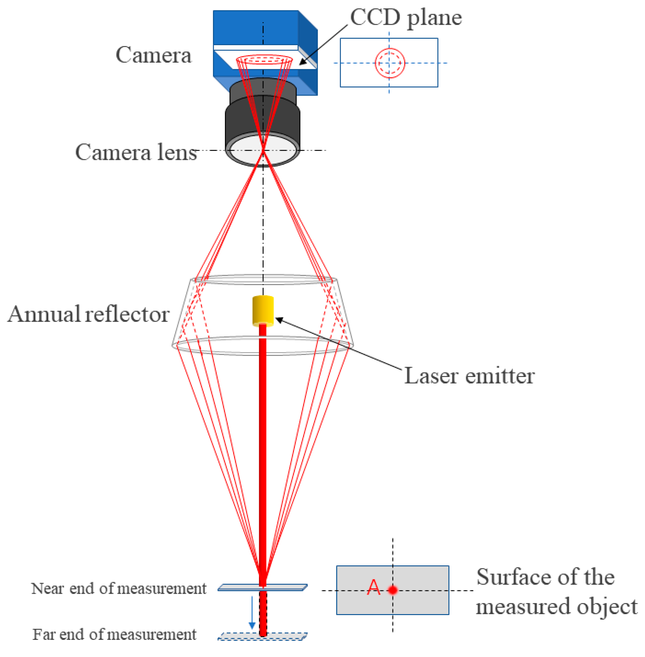
2. The Measurement Model of a Laser Triangulation Displacement Sensor Based on a Cylindrical Annular Reflector

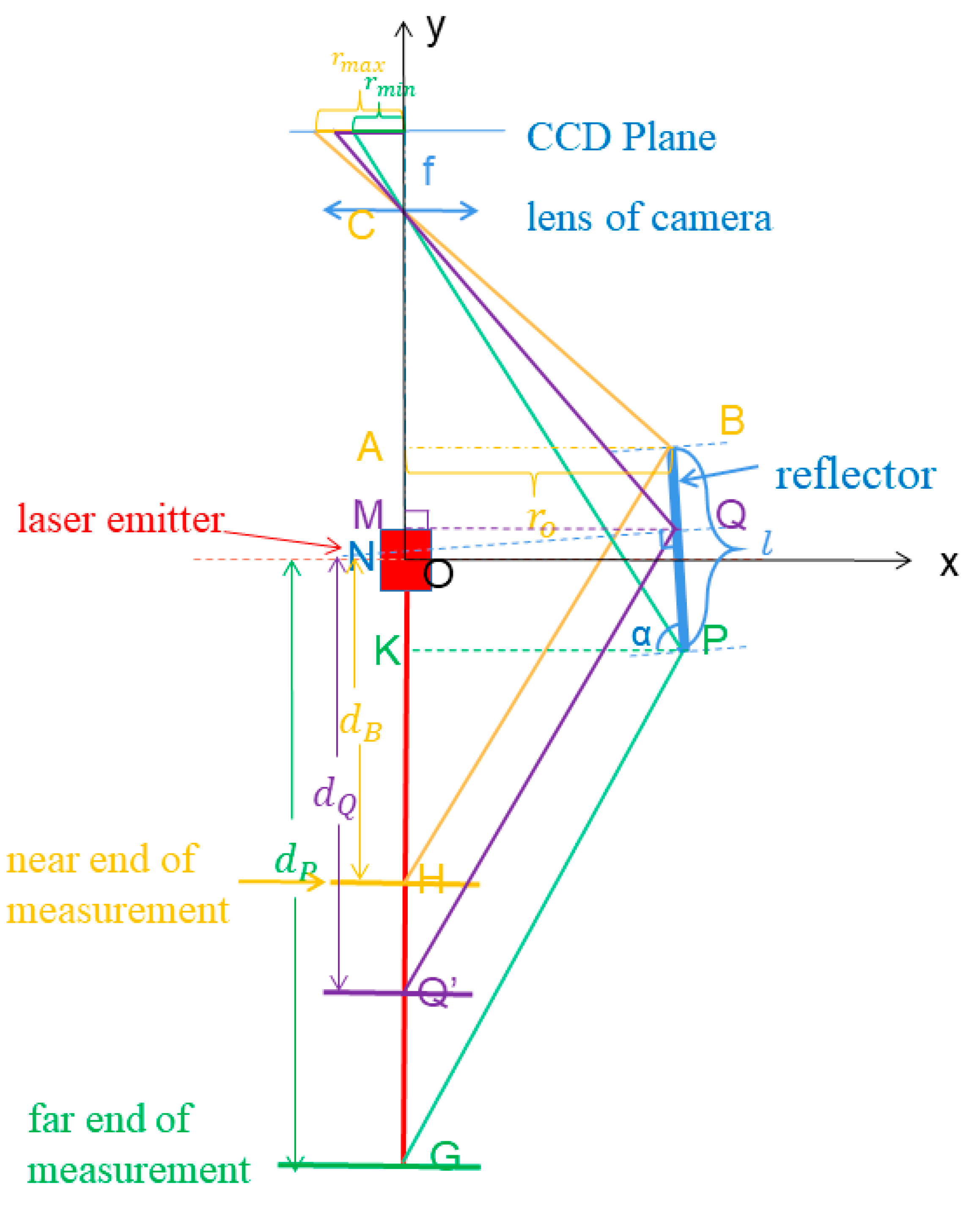
2.1. The Measurement Principle and the Mathematical Model

The Figure 1 illustrates the measurement principle of the laser triangulation displacement sensor based on a cylindrical annular reflector. In this setup, a laser beam is emitted onto the surface of the measured object, generating a measurement spot A that scatters in all directions within space. Utilizing a metal annular reflector with an inner surface reflectivity exceeding 92%, the scattered light from all directions is directed towards the camera lens, forming the measurement imaging ring on the CCD plane. The measurement optical path, formed through anisotropic scattered light, is symmetrically distributed around the laser’s output optical axis, and each measurement optical path is a deformation of a traditional laser triangulation measurement optical path, which meets the Scheimpflug condition. As the measured target moves forward and backward along the optical axis perpendicular to the laser beam, the measurement spot A also moves accordingly, causing the diameter of the circular ring spot to change. Specifically, the closer the object is, the larger the imaging ring diameter, while the farther the object is, the smaller the diameter of the imaging ring.

The size of the annular reflector plays a crucial role in determining the displacement range that the sensor can measure. There are three variables associated with the annular reflector’s size: the center radius of gyration ($r_o$), the length (l), and the angle between the reflection surface on the inner wall of the reflector and the horizontal plane (α). When the angle (α) is equal to 90°, the reflector can be a cylindrical annular reflector. These three variables establish mathematical relationships with the far and near ends of measurement. The Figure 2 illustrates one possible light path for measurement.

The focal length of the camera is $f$. Additionally, it is necessary to ensure that the scattered light from the near and far ends of the measurement is reflected by the reflector and passes through the optical center C of the lens before forming a clear image on the image plane. The upper and lower ends of the circular reflector are denoted as point B and P, respectively, and the inner diameter of the reflector at point B is $r_o$. The laser emitter is positioned at the center of rotation of the circular reflector. Let Q be an arbitrary point along the line segment BP, and the angle between BP and the horizontal plane is denoted as α. Point H and G correspond to the near and far ends of the measurement, respectively. The camera’s shortest working distance is denoted as |CA|, assumed to be $d_o$, while the length of segment |BQ| is denoted as q.

$$\begin{array}{l}\tan \theta =\frac{r_{\max }}{f}=\frac{AB}{AC}=\frac{r_o}{d_o}\end{array}$$

(1)

The radius of the imaging ring formed by point H is $r_{\max }=f\cdot \frac{r_o}{d_o}$.

The geometric relationships among the points are as follows:

$$\{\begin{array}{l}KC=KA+AC=l\cdot \sin \alpha +d_o\\ PK=AB+BP\cdot \cos \alpha =r_o+l\cdot \cos \alpha \\ \tan \angle PCK=\frac{PK}{KC}=\frac{r_o+l\cdot \cos \alpha }{l\cdot \sin \alpha +d_o}=\frac{r_{\min }}{f}\end{array}$$

(2)

Then, the radius of the imaging ring formed by the far ends of the measurement G is:

$$r_{\min }=f\cdot \frac{r_o+l\cdot \cos \alpha }{l\cdot \sin \alpha +d_o}$$

(3)

As for the an arbitrary point on the reflector (Q), its coordinates can be expressed by

$$\left[\begin{array}{l}{Q}_x\\ Q_y\end{array}\right]=\left[\begin{array}{l}{r}_o+q\cdot \cos \alpha \\ \frac{l}{2}\cdot \sin \alpha -q\cdot \sin \alpha \end{array}\right],\begin{array}{cc}& \end{array}0\le q\le l$$

(4)

$$\tan \angle QCO=\frac{Q_x}{Q^{\prime }C}=\frac{r_o+q\cdot \cos \alpha }{d_o+q\cdot \sin \alpha }$$

(5)

$$r_Q=f\cdot \tan \angle QCO=f\cdot \frac{r_o+q\cdot \cos \alpha }{d_o+q\cdot \sin \alpha }$$

(6)

Among these aforementioned formulas, point B receives scattered light from the near end of the measurement, while point P receives scattered light from the far end. By applying the law of reflection $i=r$, it is possible to determine the distances between point BP and the origin of coordinates O. Let assume

$$\angle QCO=\gamma =\arctan \frac{r_Q}{f}$$

(7)

Then

$$\angle NQ{Q}^{\prime }=\angle CQN=\angle CQM+\angle MQN=({90}^{\circ }-\angle QCO)+({90}^{\circ }-\alpha )={180}^{\circ }-(\alpha +\gamma )$$

(8)

$$\angle MQ{Q}^{\prime }=\angle MQN+\angle NQ{Q}^{\prime }=({90}^{\circ }-\alpha )+[{180}^{\circ }-(\alpha +\gamma )]={270}^{\circ }-(2\alpha +\gamma )$$

(9)

$$\tan \angle MQ{Q}^{\prime }=\frac{M{Q}^{\prime }}{QM}$$

(10)

$$M{Q}^{\prime }=(r_o+q\cdot \cos \alpha )\cdot \cot (2\alpha +\gamma )$$

(11)

$$d_{Q^{\prime }}=O{Q}^{\prime }=\frac{(r_o+q\cdot \cos \alpha )}{\tan (2\alpha +\gamma )}+(q-\frac{l}{2})\cdot \sin \alpha ,\begin{array}{cc}& \end{array}\gamma =\arctan (\frac{r_Q}{f})\begin{array}{cc}\mathrm{and}& \end{array}\alpha >{90}^{\circ }-\frac{\gamma }{2}$$

(12)

The variable $d_{Q^{\prime }}$ represents the measured point that corresponds to an arbitrary point Q on the inner side of the annular reflector. The maximum value of $r_Q$ is determined by the short edge of image plane ($l_d$). Specifically, the maximum value of $r_Q$ can be equal to half of $l_d$, and their relationship can be expressed as ${\left|r_Q\right|}_{max}=\frac{l_d}{2}$

Additionally, $r_Q$ can be calculated according to

$$r_Q=f\cdot \tan \left(\arctan \frac{r_o+q\cos \alpha }{d_{Q^{\prime }}-(q-\frac{l}{2})\sin \alpha }-2\alpha \right)$$

(13)

When q = 0 or q = l, we can derive the formulas of the near or far ends of measurement, which can be expressed as $d_B$ and $d_P$, and these formulas can be expressed as:

$$\begin{array}{l}(0,d_B)=(0,\frac{r_o}{\tan (2\alpha +\arctan \frac{r_{\max }}{f})}-\frac{l}{2}\cdot \sin \alpha )\end{array}$$

(14)

$$(0,d_P)=\frac{r_o+l\cdot \cos \alpha }{\tan (2\alpha +\arctan \frac{r_{\min }}{f})}+\frac{l}{2}\cdot \sin \alpha$$

(15)

Thus, the range of displacement measurement is

$$|d_p-d_B|=\frac{(r_o+l\cdot \cos \alpha )}{\tan (2\alpha +\arctan \frac{r_{\min }}{f})}-\frac{r_o}{\tan (2\alpha +\arctan \frac{r_{\max }}{f})}+l\cdot \sin \alpha$$

(16)

In this formula, $r_{\min }$ is the radius of the imaging ring formed by point P, which can also be expressed as $r_P$, while $r_{\max }$ is the one formed by point B, which can also be expressed as $r_B$. It can be seen that the range of displacement measurement by this method is determined by the size of the annular reflector and the focal length of the lens. When the range of displacement measurement is projected, the subsequent step is to determine the size of the annular reflector ($l,r_o,\alpha$), and this work is variables optimization that will be discussed later in the paper.

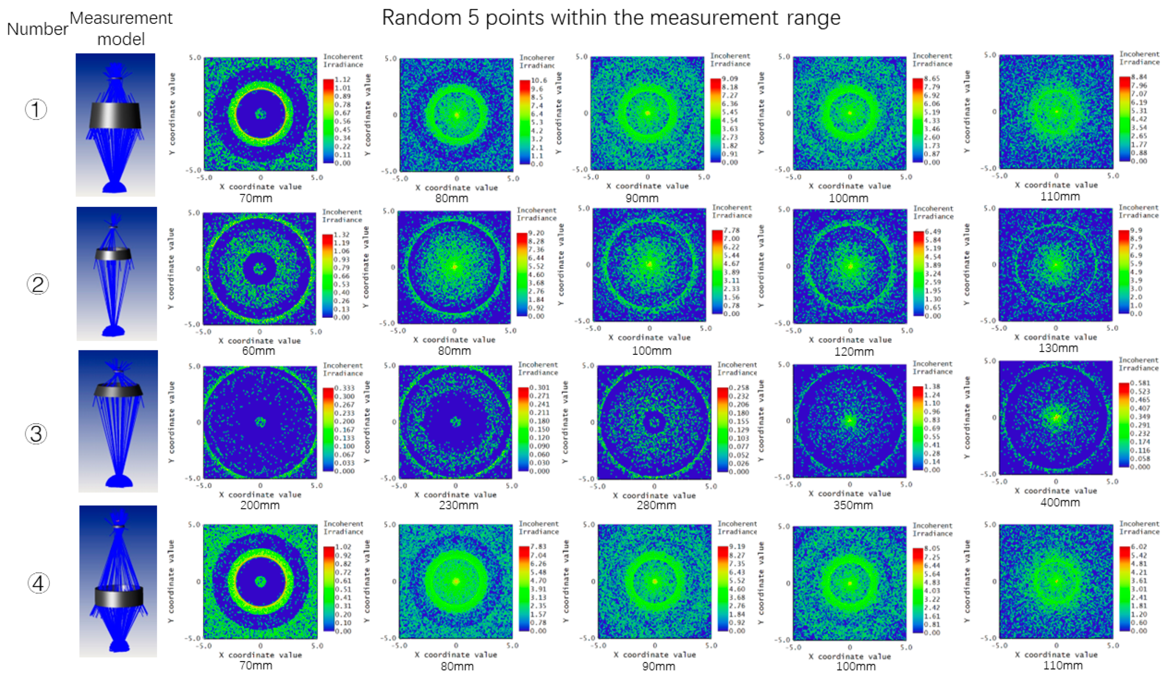
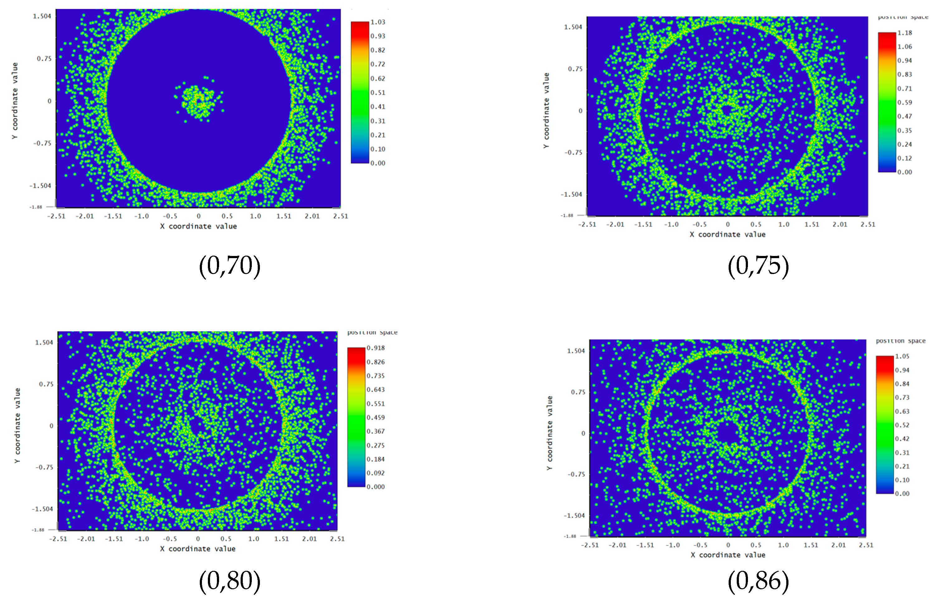
2.2. Optical Simulation

The mathematical model established above is founded on the principles of geometrical optics. In order to ascertain the feasibility of the measurement principle, it is imperative to conduct a simulation of this measurement model using Zemax software (Zemax OpticStudio 18.9). Randomly selected circular reflectors of various sizes are utilized to examine the consistency of the imaging ring radius in relation to the movement of the object being measured within the Zemax simulation. The size and position parameters of these reflectors are displayed in the

Table 1. The variables of randomly chosen reflectors.

Number	The Inner Diameter of Reflector (${\mathit{r}}_{\mathit{o}}$)	The Length of the Reflector (l)	The Angle of Inner Mirror Wall (α)	The Focal Lens of Camera’s Lens (f)	The Distance between the Lens Center and O
①	30 mm	40 mm	84°	5 mm	60 mm
②	30 mm	20 mm	80°	5 mm	40 mm
③	40 mm	20 mm	70°	5 mm	40 mm
④	40 mm	20 mm	90°	5 mm	90 mm

. Moreover, when the size of the reflector is altered, it is necessary to adjust the distance between the center of the camera lens and the origin point of the measurement system (denoted as O) to achieve clear imaging.

The non-sequential mode of Zemax is commonly employed in the design of lighting systems and performs stray light analysis on the imaging system, as well as for conducting stray light analysis on imaging systems. Additionally, a detective viewer is the most important analysis tool in this mode, which can show the results of the lighting trace. In this mode, light rays can be traced based on the principles of physical optics to determine whether they will arrive at some surfaces or objects. Additionally, a single light ray can also undergo reflection, and refraction scattering to split into multiple subrays that can also be traced simultaneously, which explains why there exists some scatter points on the imaging plane of the detective viewer. The following results of simulation in Figure 3 using four different reflectors, respectively, show the consistent variation in the change in the imaging ring’s diameter as the measured object moves.

It is evident that the diameter of the imaging ring exhibits a decreasing trend as the measured object moves from the near end to the far end within the measurement range. When $\alpha ={90}^{\circ }$, the formula for calculating $r_Q$ can be simplified as

$$r_Q=f\cdot \frac{r_o}{d_{Q^{\prime }}-q+\frac{l}{2}}$$

(17)

If the numerical values of $r_o$, $l$, and $f$ are determined, the relationship between $r_Q$ and $d_{Q^{\prime }}$ can be approximated as an inverse proportional function. Furthermore, if the parameters of the reflector’s size are chosen properly, the relationship between $r_Q$ and $d_{Q^{\prime }}$ can be liner.

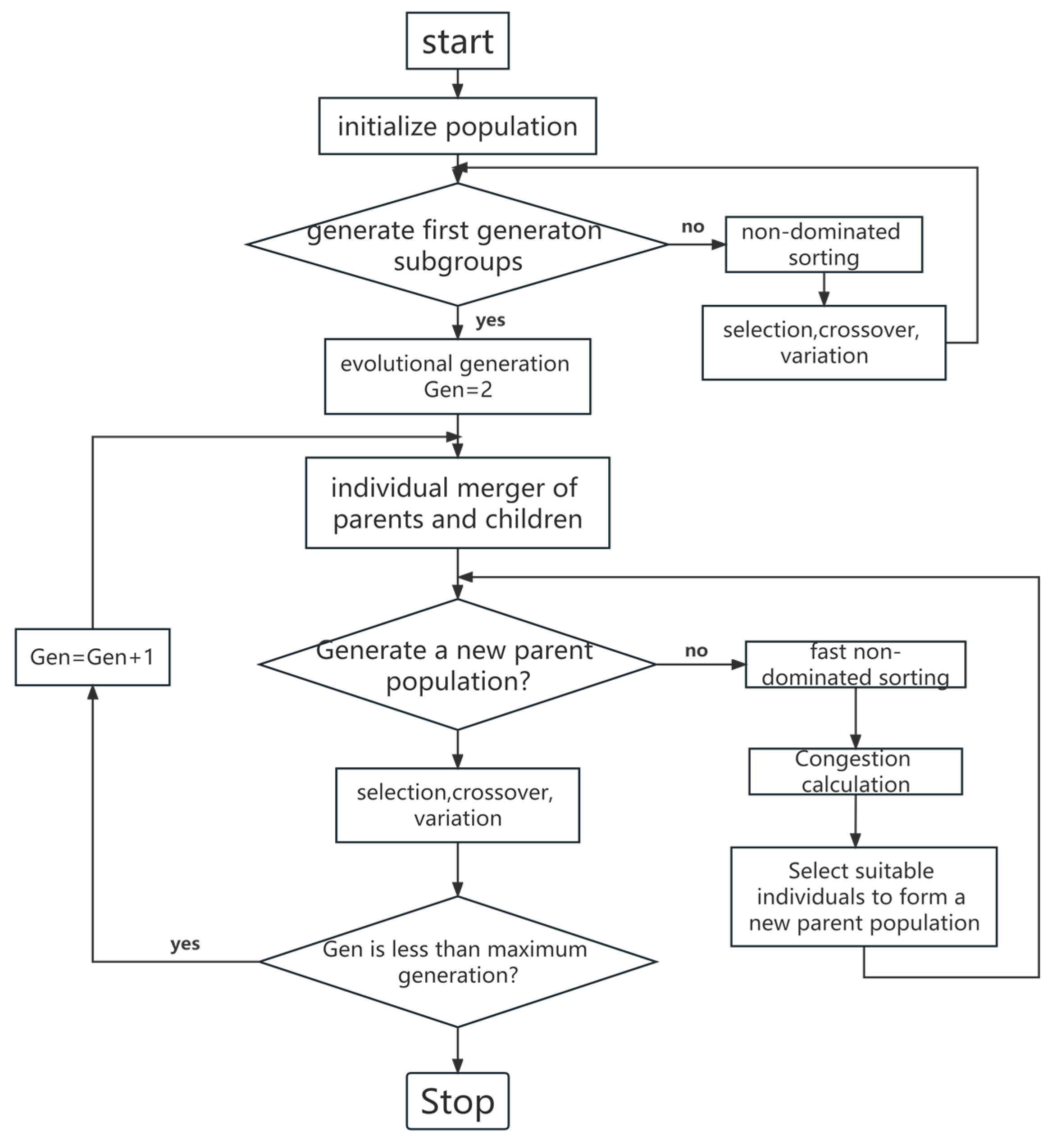
2.3. Optimization of Optical Path Parameters Depending on Measurement Sensitivity

The sensitivity of the sensor is a crucial index to evaluate its measurement accuracy. It refers to the relationship between the corresponding change in output quantity and the change in input quantity when the sensor operates in a normal and stable measurement environment. In general, sensors with higher sensitivity exhibit greater responsiveness to variations in input signals, enabling more precise measurements. According to the Formula (11), the radius of the imaging ring is closely related with the parameters of the reflector’s size ($l,r,\alpha$). Thus, optimization of the parameters of the reflector’s size is not only crucial for establishing an effective measurement system, but also for maximizing the sensor’s sensitivity, ultimately maximizing the target function K.

$$K=\frac{|r_{\max }-r_{\min }|}{|d_P-d_B|}$$

(18)

The influence of reflector size on measurement sensitivity is investigated using the control variates method. In the condition that the distance between camera and reflector is certain. When the reflector’s $r_o$ and $l$ is determined, the sensitivity K will increase by the increase in the reflector’s inner angle α. However, if the numerical values of $r_o$ and $l$ are the same, the measurement may be invalid as the near ends of the measurement are enclosed within the reflector cavity. Hence, the inner diameter of the reflector must exceed the length of the reflector. Moreover, when $l$ is maintained as a constant, the sensitivity K will be higher with the increase in $r_o$, while maintaining the same value of $r_o$, K will be lower as the increase in $l$. The three curves in Figure 4 illustrate these trends respectively.

The Genetic Algorithm (GA), inspired by Darwin’s Evolutionary Model, simulates the target question as a biological evolution process. Initially, the GA assumes the initial population as the set of hypothetical solutions to the problem. It then performs selection, crossover and mutation operations on individuals sequentially, while calculating fitness based on the selection principle of fitness. The algorithm continues until the termination criterion is met, at which point the individual is outputted, yielding a set of local optimal solutions. Over time, these solutions evolve into individuals with higher fitness function values, ultimately reaching the optimal solution for the objective function. This algorithm is commonly employed to solve a set of parameters in multi-objective optimization problems, achieving the optimal design index under a series of related constraints. The Non-dominated Sorting Genetic Algorithm (NSGA), introduced in 1995, is a variant of the GA that uses Pareto Optimality. Before the selection operator is executed, NSGA performs a layering process based on the dominance relationship between individuals. Subsequent operations, such as selection, are then performed. However, the NSGA-II algorithm [20] incorporates an elite strategy on this basis, which involves all individuals of parents and children before conducting non-dominated sorting. NSGA-II is commonly used for solving multivariate optimization problems, and the process is as shown in following Figure 5:

Due to the complexity of the Formula (17), it is difficult to solve the numerical value according to its monotonicity. Therefore, to obtain the suitable numerical values of the reflector’s $l,r_{\mathrm{o}},\alpha$ that decide measurement sensitivity K, it is helpful to use the NSGA-II algorithm combined with boundary conditions to obtain the set of optimal solutions of the reflector’s size, and then take integer results [21,22,23].

Here are the boundary conditions of these targets:

• Meet the target displacement measurement range—$|d_P-d_B|$ ≥ target displacement measurement range.
• The difference between the radius of the imaging rings formed by the near and far ends of measurement needs to be less than the half of the imaging plane’s short edge ($l_d$).
• Imaging angle γ is less than the camera’s minimum field of view angle.
• The near end of the measurement cannot be inside the cavity of the reflector in order to measure successfully, $|d_B|\ge \frac{l}{2}\cdot \cos \alpha .$

Through the iterative calculation of the NAGA-II algorithm, a solution set related to the three target values can be obtained, and then the parameters in the solution set are actually brought into the measurement model for calculation and simulation verification one by one to determine the unique solution.

3. Preparation of the Experiment and Design of Image Processing

3.1. The Model of Pixel-Measurement Depth

Combined with the research objectives of this paper, the parameters can be chosen based on the analysis of how the reflector’s size influences the measurement sensitivity and the algorithm of optimizing numerical values of the reflector’s size. The table below represents the parameter values, with the CMOS resolution set at 2592 × 1944 and a minimum pixel size of 2.2 μm.

The relationship equation between the depth of the measured object point Q′ and the radius of the imaging ring is as follows using these data

$$d_{Q^{\prime }}=\frac{(52+q)}{\tan (\frac{r_Q}{5})}+(q-5.5),0\le q\le 11$$

(19)

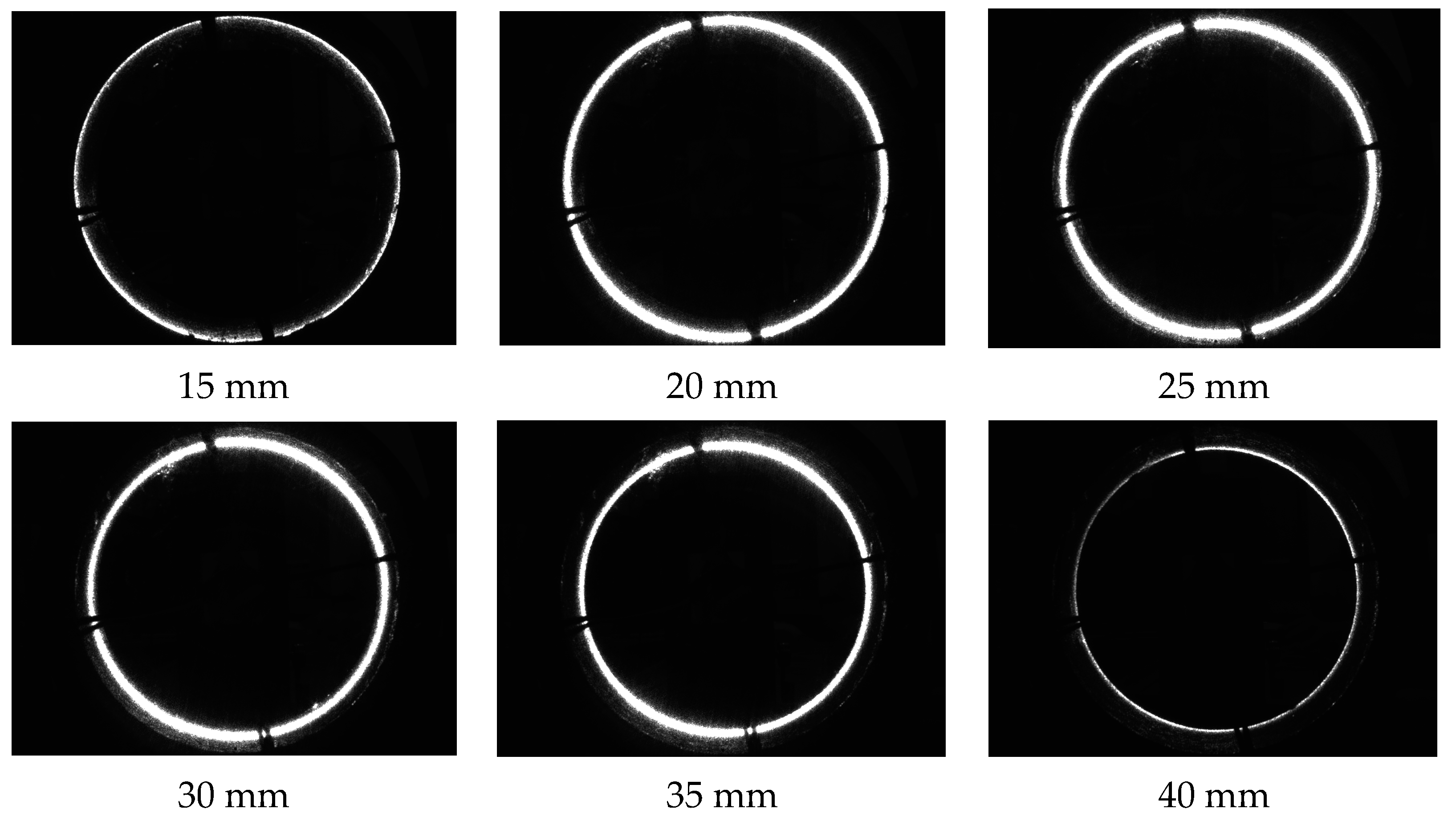
3.2. Optical Path and Imaging Characteristics

To determine whether the measure system can work using the aforementioned parameters, an optical simulation should be conducted before the experiment. In Zemax OpticStudio, a Gaussian light source with a wavelength of 650 nm is selected as the laser light source. The light source includes 500 array rays and 5 × 10⁵ analysis rays. The measured object is modeled as a Lambert surface, capable of ideal diffuse reflection (with a Lambert scattering coefficient of 1). The optical lens has a focal length and diameter of 5 mm. The detective viewer in Zemax serves as the imaging plane, set at a resolution of 2592 × 1944. A cylindrical annular reflector with an inner diameter of 52 mm, length of 11 mm, and an inclination angle of 90° between the inner wall and the horizontal plane is designed in Solidworks and then imported into Zemax. The inner wall of the reflector is constructed using MIRROR material. By inputting these system parameters into Zemax, a simulation optical path is established. The resulting simulation system, depicted in the Figure 6a, demonstrates different colored lines representing light following distinct paths. The laser beam interacts with the surface of the measured object, generating scattered light rays in all directions of space. Then, scattered rays enter the inner wall of the reflector and undergo reflection. A portion of the light is then captured on the detector viewer through the optical lens, resulting in the formation of the imaging ring on detective viewer.

Figure 6b displays the imaging on the imaging plane of detective viewer (in pseudo color) and depicts the light intensity distribution within the image. It can be seen that a circular ring spot is formed, which corresponds to the circular spot associated with the Q′ point in the pixel depth model. Additionally, scattered light from the surface of the measured object generates some scattering spots in the image. However, these spots can be filtered out without impacting the detection of the imaging ring spot. The imaging ring spot corresponds with the near end of the measurement, with a root mean square (RMS) spot radius of 1.59763180 mm and a maximum incoherent irradiance of 2.2530 W/cm².

As the measured object moves from the near end to the far end within the measurement range, the radius of the imaging ring undergoes a transition from large to small. The series of figures presented in Figure 7 show the imaging on the detective viewer at various positions of the measured object, specifically at coordinates (0,70), (0,75), (0,80) and (0,86). These figures serve to validate the correlation between the radius of the imaging ring and the distance of the measured object from the origin point, as denoted by Formula (16).

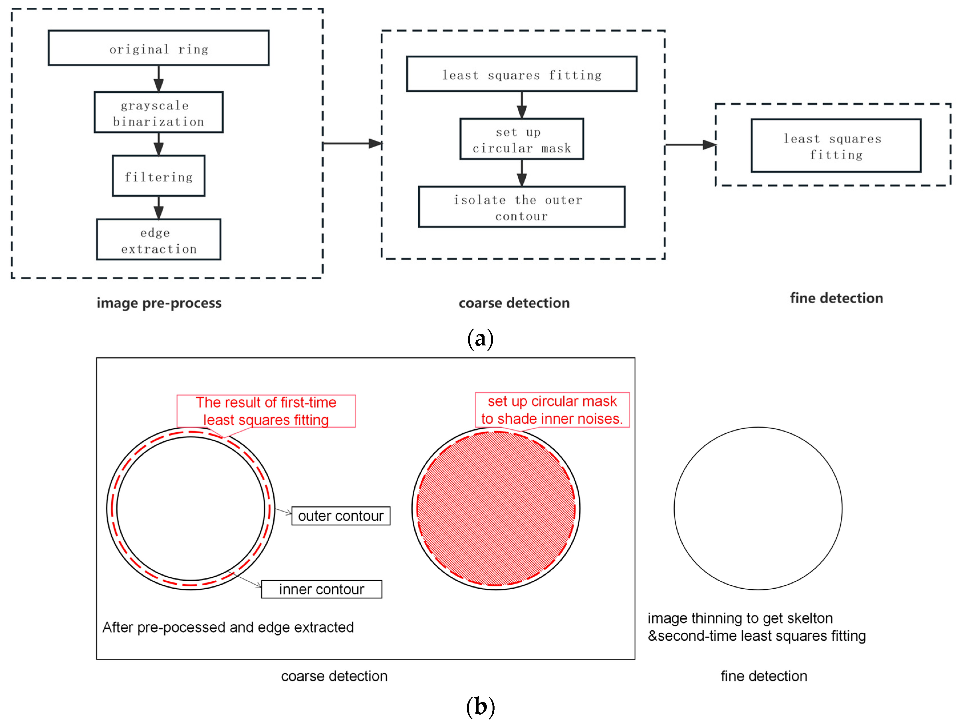
3.3. Algorithm of Image Processing

The algorithm flow for extracting the radius of the imaging ring spot obtained from this experiment is shown as in Figure 8a. This algorithm incorporates two rounds of coarse and fine detection to enhance result accuracy, which can reach the sub-pixel-level precision. After undergoing pre-processing steps such as grayscale binarization, filtering and edge extraction using a canny operator, the image is subjected to coarse detection through least squares fitting of a circle. This step provides an estimation of the imaging ring’s general position, including the coarse radius and center coordinates. Subsequently, a circular mask is created based on the numerical value of the coarse radius to eliminate interference within the ring, isolating the outer contour of the ring. The outer contour is then subjected to image thinning to generate its skeleton, which mitigates the potential errors caused by stray pixels. Finally, the processed outer contour is again subjected to least squares fitting to obtain precise measurements of the radius and center coordinates of the ring. And this process is illustrated in Figure 8b using a simplified schematic diagram.

The image thinning process for the outer contour is a mathematical morphology operation [24]. This algorithm shrinks objects to lines by removing pixels from their boundaries. The specific algorithm is as follows: 1. In the first subiteration, the pixel p is deleted only when all conditions G1, G2, and G3 are met. 2. In the second subiteration, pixel p is deleted only if all conditions, G1, G2, and G3, are met.

$$\mathrm{Condition}1:X_H(p)=1$$

$$\mathrm{where}{X}_H(p)={\displaystyle \sum }_{i=1}^4{b}_i$$

$$b_i=\left\{\begin{array}{l}1,if{x}_{2i-1}=0and(x_{2i}=1or{x}_{2i+1}=1)\\ 0,otherwise\end{array}\right\}$$

(20)

x₁, x₂,…, x₈ are the values of the eight adjacent points of p, numbered counterclockwise starting from the adjacent points on the east side.

$$\mathrm{Condition}2:2\le \min \{n1(p),n2(p)\}\le 3$$

$$\mathrm{Where}\begin{array}{l}n1(p)={\displaystyle {\displaystyle \sum }_{k=1}^4}{x}_{2k-1}\vee x_{2k}\\ n2(p)={\displaystyle {\displaystyle \sum }_{k=1}^4}{x}_{2k}\vee x_{2k+1}\end{array}$$

(21)

$$\mathrm{Condition}3:(x_2\vee x_3\vee \overline{x_8})\wedge x_1=0$$

(22)

$$\mathrm{Condition}4:(x_6\vee x_7\vee \overline{x_4})\wedge x_5=0$$

(23)

These two subiterations together form one iteration of the simplification algorithm. When an infinite number of iterations (n = Inf) are specified, the iteration will continue until the image no longer changes. This algorithm can refine the circle within the ROI into a line, and then we perform least squares circle fitting on it, shortening the iteration points for circle fitting while improving detection accuracy.

4. Experiment

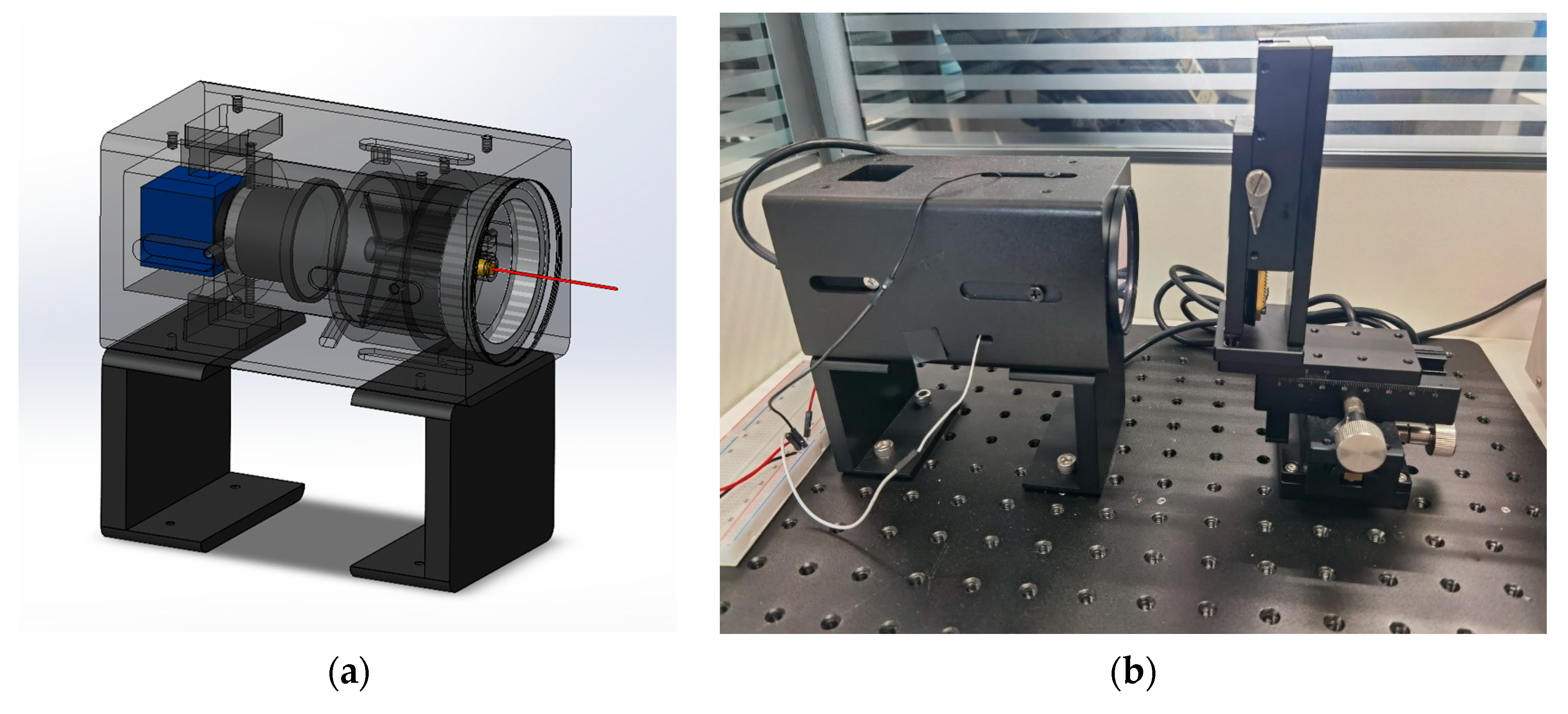
4.1. Setting of the Experiment Platform and Prototype

The validity of the measurement methodology and system is verified through a mathematical model and Zemax simulation. In order to conduct experimental testing, a physical optical path model is established by optimizing the variables involved. During this experiment phase, the imaging lens chosen is the Computar H0514-MP2 (Japan), which possesses a focal length of 5 mm. Additionally, the Daheng-Imavision MER-500-7UM camera is utilized, equipped with a 1/2.5-inch CMOS sensor chip for image capture. The cylindrical annular reflector is made of metal aluminum, with an inner wall reflectivity of over 94%, details of its shape parameters can be found in

Table 2. The values of parameters chosen.

Parameters	Value	Parameters	Value
Reflector’s inner diameter ${\mathit{r}}_{\mathit{o}}$/(mm)	52	Coordinates of near end of measurement	(0, 64)
Reflector’s length l/(mm)	11	Coordinates of far end of measurement	(0, 86)
The angle between reflector’s inner wall and horizonal plane  $\alpha$/(°)	90	Imaging ring’s maximum radius/(mm)	1.8705035971
Focal length of camera f/(mm)	5	Imaging ring’s minimum radius/(mm)	1.6149068323
The distance between camera’s center and laser emitter/(mm)	75	Measurement sensitivity K	0.01161803476

. To serve as the output laser generator, a 650 nm–5 mw laser module with a working voltage range of 3.5–5 v is selected and positioned at the center of the cylindrical annular reflector. The measured object, capable of Lambert scattering on its surface, consists of an alumina ceramics layer affixed to an XYZ 3-axis guided fine-tuning rail, enabling vertical movement along the path of the laser. Each component is mounted on the optical support to form the complete system, as depicted in Figure 9.

The validation device is used for experiments and a large number of experimental images are collected. Among these images, the regularity of the radius of the imaging ring is consistent to the results of methodology and simulation. The radius of the imaging ring will gradually decrease as the measured object moves from the near end of the measurement to the far end of the measurement. There are some experiment images shown in Figure 10.

Despite the hardware design constraints, such as the presence of small gaps in the ring, the observation of changes in the size of the imaging ring remains uninhibited. Moreover, due to the unknown optical center position of the lens, there may be some discrepancies in the relative positions between various components in actual experiments compared to simulation experiments. Additionally, the edge of the spot may be somewhat rough due to the scattering light because of the lack of optical filter in this system. However, according to the verification experiment, it is possible to identify the optimized positions of each component to design an integrated experimental prototype that can stabilize their positions, thereby enhancing measurement accuracy.

The sketch of prototype is presented in the Figure 11. To ensure alignment, the prototype utilizes the rotatability of body holes to ensure that the centers of the installed components are situated along the same horizontal and straight line. It also employs the positioning surface within the holes to maintain the relative positions between the components. To secure the reflector and laser emitter, a rotating mirror frame is designed, which can be placed within the prototype’s cavity. The lens and camera can also be securely fixed inside the cavity. Furthermore, screw holes are provided at the laser output end to facilitate the installation of optical filters. A filter with a bandwidth of 650 ± 15 nm is selected to eliminate stray light from the environment and minimize the impact of ambient light on the experimental results.

The prototype is securely mounted on the optical breadboard, while the alumina ceramics is affixed to the three-axis precision sliding table. Repetitive experiments are performed by manipulating the movement of the measured object along the direction of the laser output using the x-axis sliding table. This enables displacement changes in the measured object, as illustrated in the figure above.

4.2. Single-Point Repeatability Measurement Experiment

Repeatability is an important indicator for measuring the static properties of a sensor, which refers to the degree to which the output characteristics of the sensor are inconsistent when multiple measurements are made in the same direction within the entire measurement range. The repeatability index can be calculated using standard deviation.

$${\delta }_R=\pm \frac{(2\sim 3){\sigma }_{\max }}{Y_{FS}}\times 100\%$$

(24)

where $(2\sim 3)$ represents the confidence interval and ${\sigma }_{\max }$ is the maximum standard deviation of each point. The standard deviation of each point can be obtained using the Bessel formula.

$$\sigma =\sqrt{\frac{{\displaystyle \sum _{i=1}^n{(y_i-\overline{y})}^2}}{n-1}}$$

(25)

Additionally, n means the number of measurements.

The measurement range of the prototype is the front end face, spanning from 10 mm to 29 mm. At each location, a set of 20 image frames is captured at 1 mm intervals to serve as the data. The experimental data are recorded by repeating the process 4–6 times, starting from the near end and moving towards the far end using the x-axis guide rail. The images presented in Figure 12 are a selection of imaging ring samples.

Afterwards, image processing is conducted on each figure to fit a circular ring and determine its radius. The average value of the 20 figures is considered as the result for a specific position, along with the calculation of the uncertainty associated with the spot radius. A selection of these results is displayed in the Figure 13.

The figures show that there is a linear relationship between the radius of the imaging ring and the displacement of the measured object. The two-step detection algorithm of imaging processing proposed in 3.3 achieves a repeatability of below 0.02% for the results. In particular, when compared to the results obtained using least squares fitting once, the repeatability is significantly improved, which confirms that the algorithm proposed in this paper is effective and can achieve good results.

5. Discussion

In juxtaposition with earlier iconic studies, there has been a marked improvement in measurement repeatability. Taking Gao’s measurement model [25] as an example, they delineated a measurement range of 16 mm, and impressively managed to achieve an uncertainty (standard deviation) of less than 1 um. Furthermore, the repeatability they reported was below 0.01875%. Intriguingly, the measurement model elucidated in this study stands out as being more streamlined and pragmatic to operationalize, yet without compromising on the commendable level of measurement accuracy. On the other hand, Zhang’s exploration [19] ventured into using two measurement systems, each tailored for displacement ranges of 4.7 mm and 5.1 mm, respectively. The recorded standard deviations for his two systems were less than 0.018 and 0.015 pixels, respectively, leading to the associated uncertainties of less than 1.7 μm and 1.6 μm. As a direct upshot, the repeatability anchored by his findings hovered below 0.1085% and 0.0941%. Evidently, and quite noteworthy, is the fact that the repeatability stemming from our results decidedly eclipses that of Zhang’s findings.

6. Conclusions

In this paper, a scheme of an ultra-precision laser displacement sensor is proposed. Employing a metal cylindrical annular mirror, this sensor notably mitigates the impact of laser direction jitter on measurement outcomes. The measurement accuracy of the sensor is thoroughly investigated through the establishment of mathematical measurement models, verification of measurement principles by simulation experiments, and repeated physical experiments. Subsequent to parameter optimization, a prototype encompassing a measurement range of 20 mm is meticulously designed.

Distinctly, when compared to prior rotationally symmetric laser displacement sensors, the sensor structure in this paper boasts a more streamlined architecture. This is because the annular reflector employed is not only elementary in its design but also facile to manufacture, positioning it as an appealing candidate for broad-scale deployment. In terms of image processing, the two-step detection algorithm proposed in this paper effectively overcomes the influence of speckle and noise by coarsely and finely detecting the imaging ring, resulting in sub-pixel-level detection results. In comparison to the traditional method that solely relies on least squares fitting, this algorithm remarkably reduces the repeatability error of the results. It maintains the repeatability error below 0.02% at all positions within the measurement range, thereby greatly improving measurement accuracy. Furthermore, it is necessary to conduct further research on the displacement measurement accuracy performance of the sensor for different surfaces in order to enhance its applicability.

In conclusion, the experiments conducted in this study primarily investigate the potential linear relationship between the imaging of the sensor and the displacement of the measured object, while we further evaluate the repeatability of the sensor’s functionality, aiming to gauge its prowess in ascertaining displacement with unwavering stability, reliability, and accuracy. In our subsequent work, a detailed analysis of the sources of error for this sensor beckons, focusing specifically on the impact of component misalignment on measurements. Accordingly, we aspire to propose methods for error compensation.

References

1. Wang, Y. Laser precision ranging technology. Spacecr. Recovery Remote Sens. 2021, 42, 22–33. (In Chinese) [Google Scholar]
2. Zhuojiang, N.; Wei, T.; Hui, Z. Development of a small-size laser triangulation displacement sensor and temperature drift compensation method. Meas. Sci. Technol. 2021, 32, 095107. [Google Scholar]
3. Xin, M.; Li, B.; Li, L.; Lan, M.; Wei, X. Measurement techniques for complex surface based on a non-contact measuring machine. Int. J. Adv. Manuf. Technol. 2022, 121, 6991–7003. [Google Scholar] [CrossRef]
4. Kienle, P.; Batarilo, L.; Akgül, M.; Köhler, M.H.; Wang, K.; Jakobi, M.; Koch, A.W. Optical setup for error compensation in a laser triangulation system. Sensors 2020, 20, 4949. [Google Scholar] [CrossRef] [PubMed]
5. Cai, Z.; Jin, C.; Xu, J.; Yang, T. Measurement of potato volume with laser triangulation and three-dimensional reconstruction. IEEE Access 2020, 8, 176565–176574. [Google Scholar] [CrossRef]
6. Huang, H.; Ni, J.; Wang, H.; Zhang, J.; Gao, R.; Guan, L.; Wang, G. A novel power stability drive system of semiconductor Laser Diode for high-precision measurement. Meas. Control 2019, 52, 462–472. [Google Scholar]
7. Dong, Z.X.; Guo, R.J.; Sun, M.N.; Xu, W. Study on dip error compensation model of laser displacement sensor and its application in measurement of spiral curved surface profile. Opt. Eng. 2022, 61, 054105. [Google Scholar]
8. Jiang, L. Laser Triangulation Displacement Measurement System with Dual-Lens Symmetric Compensation. Master’s Thesis, Zhejiang University, Hangzhou, China, 2017. (In Chinese). [Google Scholar]
9. Zhang, X.; Fei, K. Discrete rotationally symmetric triangulation method and its application. J. Optoelectron. Laser 2015, 26, 1526–1535. [Google Scholar] [CrossRef]
10. Ott, P. Optical design of rotationally symmetric triangulation sensors with low-cost detectors based on reflective optics. SPIE Opt. Metrol. 2003, 5144, 350–359. [Google Scholar]
11. Ott, P.; Gao, J.; Eckstein, J.; Wang, X. A rotationally symmetric triangulation sensor with low-cost reflective optic. In Proceedings of the 2005 IEEE International Conference on Information Acquisition, Hong Kong, China, 27 June–3 July 2005; p. 5. [Google Scholar]
12. Wang, L.; Wang, X.J.; Gao, J.; Johannes, E.; Ott, P. Laser speckle simulation in rotational symmetric triangulation sensor. J. Image Graph. 2008, 13, 2414–2419. [Google Scholar]
13. Wang, L. High-Resolution 3D Information Acquisition Technology Based on Rotationally Symmetric Triangulation Vision Sensor. Ph.D. Thesis, Hefei University of Technology, Hefei, China, 2007. (In Chinese). [Google Scholar]
14. Wang, X.J. Research on Intelligent Signal Processing System for Rotationally Symmetric Triangulation Sensor. Ph.D. Thesis, Hefei University of Technology, Hefei, China, 2007. (In Chinese). [Google Scholar]
15. Wang, X.J.; Gao, J.; Wang, L.; Zhang, X.D.; Eckstein, J.; Ott, P. A robust processing method for rotationally symmetric triangulation sensor. J. Instrum. Meas. 2007, 2, 203–211. [Google Scholar] [CrossRef]
16. Eckstein, J. Optical and Mechanical Design Methods of Rotationally Symmetric Triangulation Sensor in Integrated Vision Systems. Ph.D. Thesis, Hefei University of Technology, Hefei, China, 2009. (In Chinese). [Google Scholar]
17. Eckstein, J.; Jun, G.; Ott, P. Rotationally symmetric triangulation sensor with integrated vision system. Int. J. Optomechatronics 2009, 3, 133–148. [Google Scholar] [CrossRef]
18. Zhang, H.; Zhang, Y.; Tao, W.; Zhao, H. Rotational symmetric triangulation sensor based on an object space mirror. Opt. Eng. 2011, 50, 124401. [Google Scholar]
19. Zhang, H.B.; Tao, W.; Yang, J.F.; Zhao, H. Spot displacement in rotationally symmetric triangulation sensor. J. Shanghai Jiao Tong Univ. 2012, 46, 717–721, 728. [Google Scholar]
20. Deb, K.; Agrawal, S.; Pratab, A.; Meyarivan, T. A fast elitist non-dominated sorting genetic algorithm for multi-objective optimization: NSGA-II. In Proceedings of the Parallel Problem Solving from Nature VI Conference, Paris, France, 18–20 September 2000; pp. 849–858. [Google Scholar]
21. Zhu, H.X.; Li, W.W.; Li, T.Y.; Liu, F.C.; Zhang, C.H. Interval-adaptive Genetic Algorithm for Optimization of Unconstrained Nonlinear Programming Problems. Math. Pract. Underst. 2019, 49, 110–116. [Google Scholar]
22. Zhu, H.X.; Wang, F.L.; Zhang, Y.; Zhang, F. Improved Genetic Algorithm for Optimization of Nonlinear Programming Problems. Math. Pract. Underst. 2013, 43, 117–125. [Google Scholar]
23. Wang, Y. Solving Constrained Nonlinear Programming Problems with Genetic Algorithms in MATLAB. J. Harbin Bus. Univ. (Nat. Sci. Ed.) 2006, 22, 116–117, 122. [Google Scholar] [CrossRef]
24. Lam, L.; Lee, S.W.; Suen, C.Y. Thinning Methodologies-A Comprehensive Survey. IEEE Trans. Pattern Anal. Mach. Intell. 1992, 14, 879. [Google Scholar]
25. Gao, J.; Wang, X.; Eckstein, J.; Ott, P. High precision ring location for a new rotationally symmetric triangulation sensor. Int. J. Inf. Acquis. 2005, 2, 279–289. [Google Scholar]
Figure 1. The measurement principle.
Photonics 10 01139 g001
Figure 2. A measurement light path.
Photonics 10 01139 g002
Figure 3. The consistent variation in the imaging ring’s diameter.
Photonics 10 01139 g003
Figure 4. The influence of reflector size on measurement sensitivity.
Photonics 10 01139 g004
Figure 5. The process of the NSGA-II algorithm.
Photonics 10 01139 g005
Figure 6. (a) The measurement system; (b) the imaging ring on detective viewer.
Photonics 10 01139 g006
Figure 7. The imaging on different coordinates.
Photonics 10 01139 g007
Figure 8. (a) The process of two-step detection algorithm. (b) A simplified schematic diagram to aid in understanding the algorithm.
Photonics 10 01139 g008
Figure 9. The system of verification experiment.
Photonics 10 01139 g009
Figure 10. Part of the imaging rings on CCD plane, respectively shot at distances of 15 mm, 20 mm, 25 mm, 30 mm, 35 mm and 40 mm from the end face of the reflector closest to the measured object.
Photonics 10 01139 g010
Figure 11. (a) The sketch of prototype. (b) The physical experimental prototype.
Photonics 10 01139 g011
Figure 12. A selection of imaging rings. The corresponding measurement range is from 10 mm to 29 mm, with each image representing a specific position.
Photonics 10 01139 g012
Figure 13. (a) The radius of the imaging rings. (b) The repeatability of the radius.
Photonics 10 01139 g013