Optimal Orientation Angle Configuration of Polarizers Exists in a 3 × 3 Mueller Matrix Polarimeter

Abstract

A 3 × 3 Mueller matrix polarimeter, as one of the primary polarization measurement tools, has attracted intensive interest in various fields of polarization optics. In this paper, from a novel viewpoint with more mathematical analysis of the basic configuration and the working performance of a 3 × 3 Mueller matrix polarimeter, we systematically study the relationship between Mueller matrix measurement errors with the configuration and characteristics of polarizers in the polarimeter. We figure out that, mathematically, there is an optimal orientation angle configuration (0°, 60°, and 120°) of polarizers, which inherently ensures a minimal relative measurement error in general. Moreover, we interpret the internal source of such a robust error resistance under this optimized configuration mathematically for the first time. Simulation and practical experiments show the effectiveness of our mathematical analyses, and compared to the frequently used orientation angle configuration, the average relative error is reduced by up to 32% under such an optimized configuration.

1. Introduction

As a key dimension of optical information, polarization has received extensive attention. Optical measurement techniques based on polarization detection mainly focus on interactions between objects and polarized light. Because of the sensitivity of polarization states to morphological characteristics and physical and chemical properties of an object, polarimetry is applied as a precision measurement technology in various fields, such as cancer detection [1,2,3], characterization of biological tissue [4,5,6,7], defect inspection [8,9], etc.

In general, a polarization state can be represented by a Stokes vector in mathematics, which is a four-dimensional real vector. Linear transformation of polarization states caused by an object is described by a Mueller matrix (MM), which is a real matrix with a size of 4 × 4. There is a lot of useful information that could be extracted from the MM. For example, one can characterize the diattenuation, depolarization, and retardance of an object via Mueller matrix polar decomposition [10,11]. On the other hand, 3 × 3 MM as a submatrix of 4 × 4 MM has attracted intensive interest recently. Compared to 4 × 4 MM, 3 × 3 MM only characterizes the linear polarization characteristics of an object, which can be measured by a relatively simplified MM polarimeter that only has a pair of rotatable polarizers without waveplate. Therefore, 3 × 3 MM polarimetry is usually applied in scenarios where the complexity of optical setup is limited, such as endoscopy [12,13].

As the cornerstone of MM polarimetry, the MM polarimeter has become an essential instrument to measure the MMs of samples. In general, a 3 × 3 MM polarimeter is simple and consists of a pair of rotatable polarizers. Therefore, the orientation angle and the extinction ratio of polarizers are two important parameters that could be optimized for minimizing the measurement errors of a polarimeter as much as possible. Although optimal designs of 4 × 4 polarimeters have been widely discussed by previous works [14,15,16], similar designs of 3 × 3 polarimeters are rarely discussed. In the past few years, there has been solid work [17] that discussed the calibration of a 3 × 3 polarimeter, where the method used to choose an optimal combination of calibration samples is similar to the method for finding the optimal parameters of polarimeters. In this paper, the fundamental principle of a canonical 3 × 3 MM polarimeter, the measurement errors, and the dependence of which on the configurations of polarizers are discussed. Based on rigorous mathematical analysis of the polarimeter, it is found that there always exists an optimal orientation angle configuration (0°, 60° and 120°) of polarizers in the 3 × 3 MM polarimeter, which inherently ensures obtaining a robust error resistance.

In order to verify the optimality of the suggested angle configuration and the validity of the mathematical analyses, some simulations and practical experiments are conducted. The simulations show that the mathematical analyses are rigorous, reasonable, and effective, and the polarimeter with the optimal orientation angle configuration has robust error resistance for three kinds of common errors. The result of the practical experiment is in accord with the results of the simulations. The average relative error of the polarimeter is reduced by up to 32% when such an optimal orientation angle configuration is adopted.

Moreover, we also discussed an optimization of the orientation angle configuration of a frequently used oversampling 3 × 3 MM polarimeter, and the performance of the canonical polarimeter is compared to the oversampling polarimeter. It is found that although the error resistances of both polarimeters are identical in theory, the practical performance of the oversampling 3 × 3 MM polarimeter is a little bit better than the canonical polarimeter.

Other chapters of this paper are organized according to the following structure. Section 2 introduces the 3 × 3 MM of polarizers and the general mathematical model of a 3 × 3 MM polarimeter. Section 3 discusses the optimization of the polarimeter, where the optimal orientation angle configuration is suggested. Section 4 discusses the validation of the optimality of the configuration and the validity of the mathematical analyses. The effectiveness of the error analysis, the optimal orientation angle configuration of the oversampling 3 × 3 MM polarimeter, and the performance comparison between the four-states-polarimeter and the three-states-polarimeter are also discussed in Section 5. The conclusion of the paper is given in Section 6.

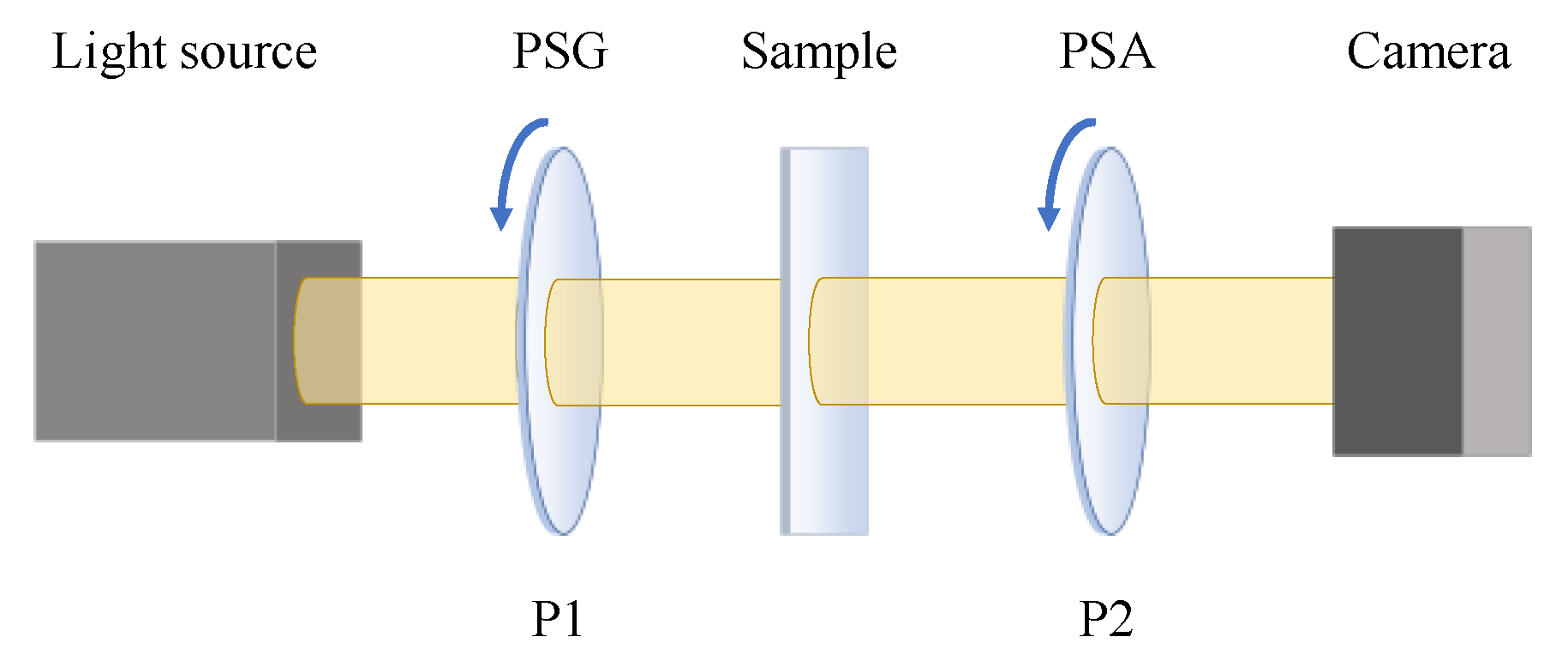
2. Principle of a 3 × 3 MM Polarimeter

2.1. The 3 × 3. MMs of Polarizers

Polarizers are the most important elements in the 3 × 3 MM polarimetry. In this subsection, 3 × 3 MMs of polarizers are briefly introduced for future discussions. As examples of diattenuators [10], 3 × 3 MMs of polarizers, denoted by M_D, can be expressed in blocks by

$$M_{\mathrm{D}}=m_{00}\left[\begin{array}{cc}1& D^{\mathrm{T}}\\ D& m_{\mathrm{D}}\end{array}\right],$$

(1)

where m₀₀ is the average intensity coefficient of M_D; D is the diattenuation vector, which is a 2 × 1 real vector and satisfies |D| ≤ 1; T denotes the transpose operation; m_D is a 2 × 2 real matrix that can be obtained by

$$m_{\mathrm{D}}=\sqrt{1-D^2}{I}_{2\times 2}+\left(1-\sqrt{1-D^2}\right)\widehat{D}{\widehat{D}}^{\mathrm{T}},$$

(2)

in which I_{2 × 2} is a 2 × 2 unit matrix; D is the diattenuation that satisfies D = |D|; $\widehat{D}$ is the normalized diattenuation vector that can be obtained by $\widehat{D}$ = D/|D|. It can be deduced from Equations (1) and (2) that M_D can be fully characterized by D and m₀₀.

If D can be parameterized by D = D[cosθ sinθ]^T, 0 ≤ θ < π, the diattenuator characterized by M_D will be a linear diattenuator (or linear polarizer) with orientation angle θ. Further, if D = 1, the linear polarizer is an ideal one, which can fully extinct a beam of linearly polarized light with a polarization angle of θ ± (π/2).

The diattenuation of a polarizer can be calculated from its polarization extinction ratio ER in the following form:

$$D=\frac{\mathrm{ER}-1}{\mathrm{ER}+1}$$

(3)

As a special case, D = 1 when ER = ∞. Moreover, it can be seen in Equation (3) that D is increasing with the increase of ER when 1 ≤ ER ≤ ∞, i.e., the higher the diattenuation, the higher the extinction ratio.

2.2. Principle of 3 × 3 MM Polarimeter

A canonical 3 × 3 MM imaging polarimeter is shown in Figure 1 schematically. A fully unpolarized light as the light source of the system is modulated by a linear polarizer (P1) and then illuminates a sample. The transmitted light of the sample is modulated by another linear polarizer (P2). A camera following P2 is used to measure the intensity of the transmitted light of P2. Without loss of generality, assuming 3 × 3 MMs of P1 and P2 and the sample to be M_PSG, M_PSA, and M, respectively, then the three-dimensional Stokes vector of light transmitted through P2, denoted by s_out, can be expressed by Equation (4):

$$s_{\mathrm{out}}=M_{\mathrm{PSA}}M{M}_{\mathrm{PSG}}{s}_{\mathrm{in}},$$

(4)

where s_in is the three-dimensional Stokes vector of the light source. In a canonical 3 × 3 MM imaging polarimeter system shown in Figure 1, the light source is unpolarized; thus, s_in = [I_in 0 0]^T with I_in is the intensity of light. Note that the MMs of P1 and P2, i.e., M_PSG and M_PSA, are two known parameters, which have been described in Section 2.1. Moreover, I_in can also be assumed to be known in this work, meaning that unknown parameters in Equation (4) are only s_out and M.

As usual, P1 and P2 are known as a polarization state generator (PSG) and a polarization state analyzer (PSA), respectively. The PSG is used to generate different polarized light to illuminate the sample, while the PSA is used to analyze the polarization state of the transmitted light of the sample. For more detail, assuming that the three-dimensional Stokes vector of the transmitted light of the sample is s = MM_PSGs_in, then Equation (4) can be rewritten as

$$s_{\mathrm{out}}=M_{\mathrm{PSA}}s.$$

(5)

The first Stokes parameter of s_out, denoted as I_out, is the intensity of the transmitted light of P2 and can be measured directly by a camera. Assuming the orientation angles of the PSA and the PSG are θ_PSA and θ_PSG, respectively, it is obvious that M_PSA is relevant to θ_PSA, s is relevant to θ_PSG, and I_out is relevant to both angles. According to Equations (1) and (5), I_out satisfies the equation

$$m_{00}\left[\begin{array}{cc}1\hfill & D_{\mathrm{PSA}}^{\mathrm{T}}\left({\theta }_{\mathrm{PSA}}\right)\hfill \end{array}\right]s\left({\theta }_{\mathrm{PSG}}\right)=I_{\mathrm{out}}\left({\theta }_{\mathrm{PSA}},{\theta }_{\mathrm{PSG}}\right),$$

(6)

where D_PSA(θ_PSA) = D_PSA[cosθ_PSA sinθ_PSA]^T is the diattenuation vector of PSA and D_PSA is the corresponding diattenuation. Moreover, s and I_out in Equation (6) are the functions of θ_PSG and (θ_PSA, θ_PSG), respectively. If PSA (i.e., P2) was rotated three times and I_out was captured by the camera for each time, then linear equations about s can be built as

$$\begin{array}{l}{m}_{00}\left[\begin{array}{cc}1\hfill & D_{\mathrm{PSA}}^{\mathrm{T}}\left({\theta }_{\mathrm{PSA}}^{\left(1\right)}\right)\hfill \\ 1\hfill & D_{\mathrm{PSA}}^{\mathrm{T}}\left({\theta }_{\mathrm{PSA}}^{\left(2\right)}\right)\hfill \\ 1\hfill & D_{\mathrm{PSA}}^{\mathrm{T}}\left({\theta }_{\mathrm{PSA}}^{\left(3\right)}\right)\hfill \end{array}\right]s\left({\theta }_{\mathrm{PSG}}\right)=\left[\begin{array}{c}{I}_{\mathrm{out}}\left({\theta }_{\mathrm{PSA}}^{\left(1\right)},{\theta }_{\mathrm{PSG}}\right)\\ I_{\mathrm{out}}\left({\theta }_{\mathrm{PSA}}^{\left(2\right)},{\theta }_{\mathrm{PSG}}\right)\\ I_{\mathrm{out}}\left({\theta }_{\mathrm{PSA}}^{\left(3\right)},{\theta }_{\mathrm{PSG}}\right)\end{array}\right],\\ \mathrm{or} \mathrm{equivalently} A_{\mathrm{PSA}}s=I_{\mathrm{out}},\end{array}$$

(7)

where ${\theta }_{\mathrm{PSA}}^{\left(1\right)}$, ${\theta }_{\mathrm{PSA}}^{\left(2\right)}$ and ${\theta }_{\mathrm{PSA}}^{\left(3\right)}$ are the orientation angles of PSA for each rotation. If they were chosen to be appropriate angles, the coefficient matrix A_PSA can be invertible, meaning that s(${\theta }_{\mathrm{PSG}}$) can be solved from Equation (7). In a word, the Stokes vector of the light modulated by the sample can be measured by rotating the PSA and measuring the intensity of the transmitted light.

Further, if the PSG (i.e., P1) was rotated three times and each time the s(θ_PSG) was measured accordingly by rotating PSA as mentioned above, based on s = MM_PSGs_in and the expression of M_PSG, a matrix equation about the 3 × 3 MM of the sample, i.e., M, can be built as

$$\begin{array}{l}M\left(I_{\mathrm{in}}{m}_{00}\left[\begin{array}{ccc}1& 1& 1\\ D_{\mathrm{PSG}}\left({\theta }_{\mathrm{PSG}}^{\left(1\right)}\right)& D_{\mathrm{PSG}}\left({\theta }_{\mathrm{PSG}}^{\left(2\right)}\right)& D_{\mathrm{PSG}}\left({\theta }_{\mathrm{PSG}}^{\left(3\right)}\right)\end{array}\right]\right)=\left[\begin{array}{ccc}s\left({\theta }_{\mathrm{PSG}}^{\left(1\right)}\right)& s\left({\theta }_{\mathrm{PSG}}^{\left(2\right)}\right)& s\left({\theta }_{\mathrm{PSG}}^{\left(3\right)}\right)\end{array}\right],\\ \mathrm{or} \mathrm{equivalently} M{A}_{\mathrm{PSG}}=S,\end{array}$$

(8)

where D_PSG(θ_PSG) = D_PSG[cosθ_PSG sinθ_PSG]^T is the diattenuation vector of PSG and D_PSG is the corresponding diattenuation; ${\theta }_{\mathrm{PSG}}^{\left(1\right)}$, ${\theta }_{\mathrm{PSG}}^{\left(2\right)}$ and ${\theta }_{\mathrm{PSG}}^{\left(3\right)}$ are orientation angles of PSG for each rotation. If the three orientation angles of the PSG were appropriate, making A_PSG invertible, M can then be solved from Equation (8). In fact, according to Equation (7), the constant matrix S in Equation (8) can be obtained by

$$\begin{array}{l}{m}_{00}\left[\begin{array}{cc}1\hfill & D_{\mathrm{PSA}}^{\mathrm{T}}\left({\theta }_{\mathrm{PSA}}^{\left(1\right)}\right)\hfill \\ 1\hfill & D_{\mathrm{PSA}}^{\mathrm{T}}\left({\theta }_{\mathrm{PSA}}^{\left(2\right)}\right)\hfill \\ 1\hfill & D_{\mathrm{PSA}}^{\mathrm{T}}\left({\theta }_{\mathrm{PSA}}^{\left(3\right)}\right)\hfill \end{array}\right]S=\left[\begin{array}{ccc}\begin{array}{c}{I}_{\mathrm{out}}\left({\theta }_{\mathrm{PSA}}^{\left(1\right)},{\theta }_{\mathrm{PSG}}^{\left(1\right)}\right)\\ I_{\mathrm{out}}\left({\theta }_{\mathrm{PSA}}^{\left(2\right)},{\theta }_{\mathrm{PSG}}^{\left(1\right)}\right)\\ I_{\mathrm{out}}\left({\theta }_{\mathrm{PSA}}^{\left(3\right)},{\theta }_{\mathrm{PSG}}^{\left(1\right)}\right)\end{array}& \begin{array}{c}{I}_{\mathrm{out}}\left({\theta }_{\mathrm{PSA}}^{\left(1\right)},{\theta }_{\mathrm{PSG}}^{\left(2\right)}\right)\\ I_{\mathrm{out}}\left({\theta }_{\mathrm{PSA}}^{\left(2\right)},{\theta }_{\mathrm{PSG}}^{\left(2\right)}\right)\\ I_{\mathrm{out}}\left({\theta }_{\mathrm{PSA}}^{\left(3\right)},{\theta }_{\mathrm{PSG}}^{\left(2\right)}\right)\end{array}& \begin{array}{c}{I}_{\mathrm{out}}\left({\theta }_{\mathrm{PSA}}^{\left(1\right)},{\theta }_{\mathrm{PSG}}^{\left(3\right)}\right)\\ I_{\mathrm{out}}\left({\theta }_{\mathrm{PSA}}^{\left(2\right)},{\theta }_{\mathrm{PSG}}^{\left(3\right)}\right)\\ I_{\mathrm{out}}\left({\theta }_{\mathrm{PSA}}^{\left(3\right)},{\theta }_{\mathrm{PSG}}^{\left(3\right)}\right)\end{array}\end{array}\right],\\ \mathrm{or} \mathrm{equivalently} A_{\mathrm{PSA}}S=I.\end{array}$$

(9)

Then, according to Equations (8) and (9), the intensity matrix I can be expressed as

$$I=A_{\mathrm{PSA}}M{A}_{\mathrm{PSG}}$$

(10)

It should be noted that Equations (7) and (8) imply the two polarizers, i.e., the PSA and PSG, having the same m₀₀, meaning that we do not distinguish m₀₀ of both. This is owing to the fact that the physical properties of the two polarizers in the polarimeter tend to be the same in general, and the value of m₀₀ is not important for a relative MM polarimeter that is used to measure the normalized MM of the sample instead of the precise value of the MM. The relative MM polarimeter is the most used type of polarimeter.

According to the analyses mentioned above, in principle, the measurement of the MM of the sample can be divided into two parts; part one includes rotating the PSA, measuring the intensity, and solving Equation (7); part two includes rotating the PSG, repeating part one and solving Equation (8). Although, in practical applications, it may seem that the MM of the sample is obtained in other ways, not directly by Equations (7) and (8). For example, Ref. [12] calculates the MM by a formula that is deduced from the physical interpretation of the Stokes parameters instead of solving the equations. However, the formula they used can also be deduced from Equations (7) and (8) when ${\theta }_{\mathrm{PSG}}^{\left(1\right)}$, ${\theta }_{\mathrm{PSG}}^{\left(2\right)}$, ${\theta }_{\mathrm{PSG}}^{\left(3\right)}$ are chosen to be 0°, 45°, 90° and ${\theta }_{\mathrm{PSA}}^{\left(1\right)}$, ${\theta }_{\mathrm{PSA}}^{\left(2\right)}$, ${\theta }_{\mathrm{PSA}}^{\left(3\right)}$ to be 0°, 90°, 135°, respectively. In fact, the measurement principle discussed above has generality, which provides a general mathematical model for a 3 × 3 MM polarimeter. All the following discussions will be based on the above principle.

Because there are nine unknown elements in M, one needs to measure the intensity nine times, at least under different orientation angles of the PSA and the PSG. However, a measurement method that has been reported [13] needs to measure the intensity sixteen times for different PSG and PSA states in total to calculate the 3 × 3 MM of the sample. These methods add extra equations to Equations (7) and (8) by rotating the PSG and PSA and measuring the intensity more times. The number of equations is larger than the number of known parameters, which means the equations may be over-determined if there is noise in the measurement. In this case, one needs to use the pseudoinverse matrix to obtain M, which will be discussed in Section 5.3. On the other hand, for 4 × 4 MM polarimetry, naturally, there is a need to measure the intensity at least sixteen times since there are sixteen unknown elements in 4 × 4 MMs. There are other works [18,19] that need more times (more than sixteen times) of rotations and intensity measurements to calculate a 4 × 4 MM. These methods, essentially, build over-determined equations via multiple intensity measurements of different polarization states and usually use some numerical methods (least square method or Fourier analysis) to obtain approximate solutions to the equations. The ideas of these 4 × 4 methods also can be applied on the 3 × 3 MM polarimetry. All the polarimeters that include extra rotations and intensity measurements are referred to as oversampling polarimeters. However, the oversampling polarimeters are not within the scope of this article (except for an oversampling polarimeter discussed in Section 5.3). Fewer times of rotation and intensity measurement are conducive to reducing the cost of data processing and approving the measurement speed and timeliness.

3. Error Analysis of the MM Polarimeter

3.1. Measurement Errors in MM Polarimeter

There are three kinds of sources of errors that should be considered in the polarimeter, i.e., the instrumental errors of the PSG, the PSA, and the camera. Mathematically, although the instrumental errors of the PSG and the PSA are reflected in the errors of M_PSG and M_PSA, respectively, both of them, together with the inherent error of the camera, will be embodied in the error of the detected I simultaneously. As a result, such three kinds of errors will influence the measured MM of the sample.

It should be emphasized that all three kinds of errors will be converted to intensity errors finally. In this case, the solution of Equation (9), i.e., S, also has errors, which thus leads to the errors in M based on Equation (8). In this paper, the matrix error is defined by using the 2-norm or the Frobenius norm (F-norm). As for M, the error of which can be defined as

$$\mathrm{error}={‖M-\widehat{M}‖}_{*},$$

(11)

where $\widehat{M}$ and M are the measurement value and the ground truth of MM of the sample; operator ‖·‖_* stands for the 2-norm or the F-norm of the matrix. The reason for using the 2-norm or F-norm to define the matrix error is that the norms have some good properties for analysis and are compatible with the 2-norm of the vector, which is usually used to define the difference between two vectors (the difference is called the Euclid distance). The other reason for adopting these two norms is its invariance of orthogonal transformations: for any square matrix X and orthogonal matrix Q with the same size, the following equation always holds:

$${‖X‖}_{*}={‖QX{Q}^{\mathrm{T}}‖}_{*}$$

(12)

That means the error defined by the 2-norm or F-norm is invariant when the reference coordinate system is rotated. This is because the rotation transformations are kinds of orthogonal transformations.

It should be noted that, in many applications [12,13,20], the PSG and PSA were treated as ideal linear polarizers, meaning that we are assuming D_PSG = D_PSA = 1. However, there is a work [21] suggesting a calibration method for MM polarimeters based on precise diattenuation of polarizers, in which polarizers are treated as general nonideal linear polarizers. Without loss of generality, the PSG and PSA will be treated as nonideal polarizers in the following analyses, in which the ideal polarizers are treated as a special case.

3.2. Error Analysis of the System Composed of the PSA and the Camera

According to Section 2.2, the measurement of 3 × 3 MM can be divided into two parts. The first part aims to measure the three-dimensional Stokes vectors of the transmitted lights of the sample, i.e., the S, under three given states of PSG. Mathematically, this part is expressed by Equation (9), which, in this case, is only related to the system composed of the PSA and the camera. In fact, this system can be regarded as an independent linear Stokes polarimeter. This subsection analyzes the errors of the system composed of the PSA and the camera by analyzing the stability of Equation (9), where the impacts of the PSG are excluded.

If there are instrumental errors in the PSA, according to the discussion in Section 3.1, the intensity matrix I will involve some errors that will lead to errors in the solution of Equation (9). In this case, obviously, the error of the solution is relevant to the value of the coefficient matrix of Equation (9), i.e., A_PSA. That means there may exist an optimal orientation angle configuration of the PSA to minimize the potential error of the solution, which can be obtained from the perturbation analysis for Equation (9). The main principle of perturbation analysis is introducing perturbations into equations and analyzing the corresponding error of the solution. In the case of Equation (9), only the perturbation of constant matrix I needs to be introduced if the calculation error can be ignored. Assuming the perturbative matrix of I is ΔI, and the corresponding error of the solution S is ΔS, then the equation containing errors can be expressed as

$$A_{\mathrm{PSA}}\left(S+\Delta S\right)=(I+\Delta I),$$

(13)

where S is the precise solution of Equation (9) and satisfies A_PSA S = I. As we mentioned before, S is a matrix composed of three Stokes vectors of the transmitted lights of the sample under different states of PSG. The perturbation of I, i.e., ΔI, can be regarded as the intensity error caused by errors of the PSA and the camera. The perturbation of S, i.e., ΔS, is the error of S caused by ΔI.

In fact, we can assume that I + ΔI is the measured value of I, which satisfies

$$(I+\Delta I)=\left(A_{\mathrm{PSA}}+\Delta A_{\mathrm{PSA}}\right)S+\Delta I_{\mathrm{C}},$$

(14)

in which A_PSA + ΔA_PSA is the ground truth of A_PSA; ΔI_C is the intensity perturbation caused by the instrumental error of the camera. In fact, ΔA_PSA can be regarded as a perturbative matrix caused by the instrumental error of the PSA. In order to avoid ambiguity, it should be emphasized that there is not any perturbation added to the coefficient matrix of Equation (9), which can be seen in Equation (13). The ΔA_PSA is the difference between A_PSA and its ground truth A_PSA + ΔA_PSA; the latter is correlated to the realistic physical state of PSA. The difference ΔA_PSA is one of the reasons causing intensity error ΔI. The perturbation of the coefficient matrix in Equation (9) should be introduced only when the coefficient matrix used to solve the equations in practice may be different from its assumption (the difference is caused by calculating error in this case, but the calculating error has been ignored in this paper).

By analyzing Equations (13) and (14), an inequality can be deduced, which can be expressed as

$$\frac{{‖\Delta S‖}_{*}}{{‖S‖}_{*}}\le {\mathrm{cond}}_{*}\left(A_{\mathrm{PSA}}\right)\left(\frac{{‖\Delta A_{\mathrm{PSA}}‖}_{*}}{{‖A_{\mathrm{PSA}}‖}_{*}}+\frac{{‖\Delta I_{\mathrm{C}}‖}_{*}}{{‖I‖}_{*}}\right),$$

(15)

where cond_*(A_PSA) is the condition number of A_PSA, which is defined based on the 2-norm or the F-norm and satisfies

$${\mathrm{cond}}_{*}\left(A_{\mathrm{PSA}}\right)={‖A_{\mathrm{PSA}}‖}_{*}{‖A_{\mathrm{PSA}}^{-1}‖}_{*}$$

(16)

In Equation (15), the ratio ‖ΔA_PSA‖_*/‖A_PSA‖_* can be treated as the relative error of A_PSA. The ratios ‖ΔI_C‖_*/‖I‖_* and ‖ΔS‖_*/‖S‖_* can be interpreted in the same way. Equation (15) gives the upper boundary of the relative error of the solution of Equation (9) under a given amount of the relative instrumental errors of the PSA and the camera. It is obvious that if the relative instrumental errors of the PSA and the camera were given, the upper boundary of the relative error of the solution S is only relative to A_PSA.

At the end of this subsection, it should be noted that values of ΔA_PSA and ΔI_C are arbitrary in Equation (15), meaning that our analysis is applicable for any error sources of the PSA and the camera. For example, for PSA, both the mechanical rotation error and the depolarization error are applicable despite the fact that the latter will lead to the MM of the PSA being depolarized.

3.3. Error Analysis of the PSG

The MM of the sample can be solved from Equation (8) if the constant matrix S in Equation (8) had been solved from Equation (9). Assuming S is a known parameter, then the solution of Equation (8) is only dependent on A_PSG. Similar to the method that the error analysis of the system composed of the PSA and the camera is based on the perturbation analysis of Equation (9), the error analysis of the PSG can be fulfilled based on the perturbation analysis of Equation (8).

As we mentioned before, if there exists an error in the solution of Equation (9), i.e., S + ΔS, the MM of the sample solved from Equation (8) is also in error. Assuming that the error of the MM of the sample is ΔM, then Equation (8) in error can be expressed as

$$\left(M+\Delta M\right)A_{\mathrm{PSG}}=(S+\Delta S).$$

(17)

In this case, ΔS can be divided into two parts: the first part is the solution error of Equation (9), and the second part is the error caused by the instrumental error of the PSG. Therefore, S + ΔS can be expressed as

$$(S+\Delta S)={\rm M}\left(A_{\mathrm{PSG}}+\Delta A_{\mathrm{PSG}}\right)+\Delta S_{\mathrm{C}},$$

(18)

in which A_PSG + ΔA_PSG is the ground truth of A_PSG; ΔS_C is the solution error of Equation (9).

Similar to the analysis of the system composed of the PSA and the camera, an inequality can be deduced from Equations (17) and (18):

$$\frac{{‖\Delta M‖}_{*}}{{‖M‖}_{*}}\le {\mathrm{cond}}_{*}\left(A_{\mathrm{PSG}}\right)\left(\frac{{‖\Delta A_{\mathrm{PSG}}‖}_{*}}{{‖A_{\mathrm{PSG}}‖}_{*}}+\frac{{‖\Delta S_{\mathrm{C}}‖}_{*}}{{‖S‖}_{*}}\right).$$

(19)

Equation (19) gives the upper boundary of the relative error of the solution of Equation (8) under a given amount of the relative instrumental errors of PSG and the relative solution error of Equation (9).

3.4. Error Estimation of the MM Polarimeter

Having known that both the error of the PSG and the error of the system composed of PSA and camera will affect the final solution of M, i.e., the MM of the sample, it is necessary to discuss how these errors propagate to the MM of the sample.

By analyzing Equation (10), one can obtain the following inequality:

$$\begin{array}{c}\frac{{‖\Delta M‖}_{*}}{{‖M‖}_{*}}\le {\mathrm{cond}}_{*}\left(A_{\mathrm{PSA}}\right)\frac{{‖\Delta A_{\mathrm{PSA}}‖}_{*}}{{‖A_{\mathrm{PSA}}‖}_{*}}+{\mathrm{cond}}_{*}\left(A_{\mathrm{PSG}}\right)\frac{{‖\Delta A_{\mathrm{PSG}}‖}_{*}}{{‖A_{\mathrm{PSG}}‖}_{*}}\\ {+\mathrm{cond}}_{*}\left(A_{\mathrm{PSA}}\right){\mathrm{cond}}_{*}\left(A_{\mathrm{PSG}}\right)\left(\frac{{‖\Delta A_{\mathrm{PSA}}‖}_{*}}{{‖A_{\mathrm{PSA}}‖}_{*}}\frac{{‖\Delta A_{\mathrm{PSG}}‖}_{*}}{{‖A_{\mathrm{PSG}}‖}_{*}}+\frac{{‖\Delta I_{\mathrm{C}}‖}_{*}}{{‖I‖}_{*}}\right).\end{array}$$

(20)

A proof of Equation (20) is given in the Appendix A. Similar to Equations (15) and (19), Equation (20) gives an upper limitation of the relative MM error (RMME, i.e., ‖ΔM‖_*/‖M‖_*) under given error matrices, i.e., ΔA_PSA, ΔA_PSG, and ΔI_C. The three error matrices can be regarded as the mathematical expressions of the three error resources introduced in Section 3.1. Therefore, Equation (20) gives an error estimation to evaluate the range of RMME of the 3 × 3 MM polarimeter.

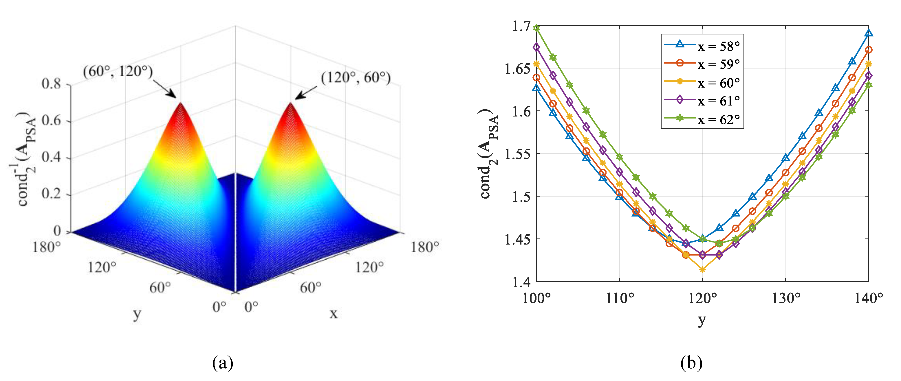
4. Optimal Design of Polarizers in MM Polarimeter

As mentioned above, it is easy to see from Equation (20) that one possible way to reduce the RMME of the 3 × 3 MM polarimeter is to minimize cond_*(A_PSA) and cond_*(A_PSG) as much as possible. Therefore, Equation (20), as the error estimation of the MM polarimeter, actually gives us a way to make an optimal design of it. A similar method is also applied in a relevant work [17] that discussed the calibration of the 3 × 3 MM polarimeter. In [17], the minimization of the condition number is used to find an optimal combination of calibration samples, where the combination of calibration samples with a minimal condition number corresponds to the minimal calibration errors. Therefore, the method has been proven effective.

Let us consider the minimization of the condition number of A_PSA. As mentioned in Section 3.1, we will only consider matrix errors defined on the 2-norm and the F-norm. The condition number of A_PSA defined on the 2-norm, denoted by cond₂(A_PSA), can be calculated from the following equation:

$${\mathrm{cond}}_2\left(A_{\mathrm{PSA}}\right)=\frac{{\sigma }_{\max }}{{\sigma }_{\min }},$$

(21)

where σ_max and σ_min are the maximal and the minimal singular values of A_PSA, respectively. Singular values of A_PSA are square roots of eigenvalues of a positive-definite matrix that is A_PSA$A_{\mathrm{PSA}}^{\mathrm{T}}$, which satisfies

$$A_{\mathrm{PSA}}{A}_{\mathrm{PSA}}^{\mathrm{T}}=m_{00}^2\left[\begin{array}{lll}{D}_{\mathrm{PSA}}^2+1\hfill & D_{\mathrm{PSA}}^2\cos \left(2x\right)+1\hfill & D_{\mathrm{PSA}}^2\cos \left(2y\right)+1\hfill \\ D_{\mathrm{PSA}}^2\cos \left(2x\right)+1\hfill & D_{\mathrm{PSA}}^2+1\hfill & D_{\mathrm{PSA}}^2\cos \left[2\left(y-x\right)\right]+1\hfill \\ D_{\mathrm{PSA}}^2\cos \left(2y\right)+1\hfill & D_{\mathrm{PSA}}^2\cos \left[2\left(y-x\right)\right]+1\hfill & D_{\mathrm{PSA}}^2+1\hfill \end{array}\right]$$

(22)

where x = ${\theta }_{\mathrm{PSA}}^{\left(2\right)}$ − ${\theta }_{\mathrm{PSA}}^{\left(1\right)}$ and y = ${\theta }_{\mathrm{PSA}}^{\left(3\right)}$ − ${\theta }_{\mathrm{PSA}}^{\left(1\right)}$. Equation (22) shows that cond₂(A_PSG) is relevant to x and y, i.e., the angle differences of ${\theta }_{\mathrm{PSA}}^{\left(2\right)}$ and ${\theta }_{\mathrm{PSA}}^{\left(3\right)}$ with respect to ${\theta }_{\mathrm{PSA}}^{\left(1\right)}$, instead of the three angles themselves. In fact, this property is caused by the invariance of orthogonal transformations of the 2-norm, which has been discussed in Section 3.1 as shown in Equation (12). Moreover, a well-known fact is that the condition number of a matrix is invariant while the matrix times a scalar coefficient. Therefore, m₀₀ can not affect cond₂(A_PSA), meaning that cond₂(A_PSA) is only relevant to x, y, and D_PSA.

Figure 2a shows a mesh surface plot of a two-dimensional distribution of ${\mathrm{cond}}_2^{-1}$(A_PSA) under D_PSA = 1 and different values of x and y in degree. Values of ${\mathrm{cond}}_2^{-1}$(A_PSA) that correspond to x = 0, y = 0, and x = y were not calculated and shown since A_PSA is singular in these cases. Moreover, Figure 2b shows one-dimensional distributions of cond₂(A_PSA) from x = 58° to x = 62° under D_{PSA =} 1 and different y from 100° to 140°. According to the results shown in Figure 2, cond₂(A_PSA) is minimized at (x, y) = (60°, 120°) under D_PSA = 1. It is worth noting that values of cond₂(A_PSA) at (x, y) are always equal to values at (y, x); therefore, cond₂(A_PSA) is also minimized at (x, y) = (120°, 60°) under D_PSA = 1. In fact, (x, y) and (y, x) are physically equivalent, which corresponds to the same orientation angles configuration of the PSA.

The results shown in Figure 2 are achieved by numerical calculations, which only give distributions of cond₂(A_PSA) under D_PSA = 1. For further exploring the effects of D_PSA on cond₂(A_PSA), we used a symbolic computation system to solve the minimum point of cond₂(A_PSA). The result of the symbolic computation shows two important properties of cond₂(A_PSA):

• Partial derivatives of cond₂(A_PSA) with respect to x and y at (x, y) = (60°, 120°) are always zeros for arbitrary D_PSA ≠ 0.
• Values of cond₂(A_PSA) at (x, y) = (60°, 120°) equal to $\sqrt{2}/\left|D_{\mathrm{PSA}}\right|$.

The two properties imply that, under a physical constrain of 0 ≤ D_PSA ≤ 1, a minimum point of cond₂(A_PSA) occurs at (x, y, D_PSA) = (60°, 120°, 1), which corresponds to a minimum value of 2^1/2.

On the other hand, the condition number of A_PSA defined on the F-norm, denoted by cond_F(A_PSA), satisfies

$$\begin{array}{l}{\mathrm{cond}}_{\mathrm{F}}\left(A_{\mathrm{PSA}}\right)=\frac{\sqrt{6}\sqrt{\left(D_{\mathrm{PSA}}^4+D_{\mathrm{PSA}}^2\right)\left(3-P_{2x,2y}\right)+4\left(D_{\mathrm{PSA}}^2+1\right)\left(3-P_{x,y}\right)}}{2\left|D_{\mathrm{PSA}}{Q}_{x,y}\right|},\\ \mathrm{where}\\ P_{x,y}=\cos \left(2x\right)+\cos \left(2y\right)+\cos \left[2\left(y-x\right)\right],\\ Q_{x,y}=\sin \left(2y\right)-\sin \left(2x\right)-\sin \left[2\left(y-x\right)\right].\end{array}$$

(23)

Similar to cond₂(A_PSA), cond_F(A_PSA) is also a function of x = ${\theta }_{\mathrm{PSA}}^{\left(2\right)}$ − ${\theta }_{\mathrm{PSA}}^{\left(1\right)}$, y = ${\theta }_{\mathrm{PSA}}^{\left(3\right)}$ − ${\theta }_{\mathrm{PSA}}^{\left(1\right)}$ and D_PSA, owing to the fact that the F-norm also has the invariance of orthogonal transformations. According to Equation (23), for arbitrary D_PSA ≠ 0, minimum points of cond_F(A_PSA) with respect to (x, y) are always at (x, y) = (60°, 120°). The corresponding minimum values of cond_F(A_PSA), denoted by min[cond_F(A_PSA), D_PSA], can be expressed as

$$\min \left[{\mathrm{cond}}_{\mathrm{F}}\left(A_{\mathrm{PSA}}\right),D_{\mathrm{PSA}}\right]=\frac{\sqrt{\left(D_{\mathrm{PSA}}^2+1\right)\left(D_{\mathrm{PSA}}^2+4\right)}}{\left|D_{\mathrm{PSA}}\right|}.$$

(24)

According to Equation (24), cond_F(A_PSA) at (x, y) = (60°, 120°) is monotonically decreasing with the increase of D_PSA from 0 to 1, meaning that a minimum point of cond_F(A_PSA) under the physical limitation of 0 ≤ D_PSA ≤ 1 occurs at (x, y, D_PSA) = (60°, 120°, 1), which corresponds to a minimum cond_F(A_PSA) of 10^1/2. This result about cond_F(A_PSA) is similar to the case of cond₂(A_PSA).

The above discussion is about cond_*(A_PSA). On the other hand, the analysis of cond_*(A_PSG) is similar to that of cond_*(A_PSA). Therefore, we directly give conclusions here: cond_*(A_PSG) is a function of x = ${\theta }_{\mathrm{PSG}}^{\left(2\right)}$ − ${\theta }_{\mathrm{PSG}}^{\left(1\right)}$, y = ${\theta }_{\mathrm{PSG}}^{\left(3\right)}$ − ${\theta }_{\mathrm{PSG}}^{\left(1\right)}$ and D_PSG; the minimum points of cond₂(A_PSG) and cond_F(A_PSG) are both occurring at (x, y, D_PSG) = (60°, 120°, 1), and the corresponding minimum values are 2^1/2 and 10^1/2, respectively.

According to the discussions above, an optimal criterion for the designation of polarizers in the 3 × 3 MM polarimeter is that

• The orientation angle configurations of the PSA and the PSG, i.e., (${\theta }_{\mathrm{PSA}}^{\left(1\right)}$, ${\theta }_{\mathrm{PSA}}^{\left(2\right)}$, ${\theta }_{\mathrm{PSA}}^{\left(3\right)}$) and (${\theta }_{\mathrm{PSG}}^{\left(1\right)}$, ${\theta }_{\mathrm{PSG}}^{\left(2\right)}$, ${\theta }_{\mathrm{PSG}}^{\left(3\right)}$), need to both satisfy the form of (c°, c° + 60°, c° + 120°), where c is an arbitrary real constant.
• Extinction ratios of the PSA and the PSG need to be as large as possible.

The criterion can minimize cond_*(A_PSA) and cond_*(A_PSG) at the same time, meaning that the MM polarimeter will have an optimal error resistance when such a criterion is fulfilled.

At the end of this section, we calculate cond_*(A_PSA) and cond_*(A_PSG) under some other orientation angle configurations and extinction ratios for reference, which are shown in

Table 1. Values of cond_*(A_PSA) and cond_*(A_PSG) under different orientation angle configurations and extinction ratios of the PSA and the PSG.

(x, y)	Extinction Ratio	cond2(APSA) and cond2(APSG)	condF(APSA) and condF(APSG)
(60°, 120°)	∞	1.4142	3.1623
(60°, 120°)	100:1	1.4428	3.1818
(60°, 120°)	10:1	1.7285	3.4124
(45°, 90°)	∞	2.4142	3.8730
(45°, 90°)	100:1	2.4489	3.8969
(45°, 90°)	10:1	2.8162	4.1794

, where x = ${\theta }_{\mathrm{PSA}}^{\left(2\right)}$ − ${\theta }_{\mathrm{PSA}}^{\left(1\right)}$ = ${\theta }_{\mathrm{PSG}}^{\left(2\right)}$ − ${\theta }_{\mathrm{PSG}}^{\left(1\right)}$, y = ${\theta }_{\mathrm{PSA}}^{\left(3\right)}$ − ${\theta }_{\mathrm{PSA}}^{\left(1\right)}$ = ${\theta }_{\mathrm{PSG}}^{\left(3\right)}$ − ${\theta }_{\mathrm{PSG}}^{\left(1\right)}$. In Table 1, the cases of (x, y) = (45°, 90°) are corresponding to orientation angle configurations of (c°, c° + 45°, c° + 90°), which are frequently used configurations [12,20].

5. Discussion

5.1. Effectiveness of the Error Analysis: A Simulation

The optimal criterion of the designation of polarizers in the 3 × 3 MM polarimeter is based on the error estimation given by Equation (20) in Section 3.4. To validate the optimality of this criterion, one needs to validate the effectiveness of the error estimation.

Equation (20) gives an upper boundary of the RMME under given amounts of the relative errors of PSG, PSA, and camera. It should be emphasized that the higher upper boundary of the RMME deduced from the perturbation analysis does not necessarily correspond to the higher RMME. Therefore, to validate the effectiveness of the error estimation, we need to confirm whether the lower upper boundary of RMME is really corresponding to the lower RMME statistically.

An intuitive method to verify the effectiveness of the error estimation is to calculate the precise RMME and its upper boundary under given relative errors of PSG, PSA, and the camera. By comparing the precise RMME to its upper boundary predicted via Equation (20), the effectiveness of the perturbation analysis can be verified: if the precise error is positively correlated with its upper limitation, then the error estimation will be effective. Considering the errors of PSG, PSA, and camera cannot be controlled precisely in practice, a numerical simulation will be conducted as an alternative.

In the simulation, we calculated the RMMEs and their upper boundaries under given samples, instrumental errors, and different orientation angle configurations to verify the effectiveness of the error estimation. The experimental samples are air and a quarter-wave plate (QWP) with an orientation angle of 45°, which are frequently used calibration samples in the calibration of the MM polarimeter [17,22]. The orientation angle configurations of the PSA and the PSG, i.e., ${\theta }_{\mathrm{PSA}}^{\left(1\right)}$, ${\theta }_{\mathrm{PSA}}^{\left(2\right)}$, ${\theta }_{\mathrm{PSA}}^{\left(3\right)}$ and ${\theta }_{\mathrm{PSG}}^{\left(1\right)}$, ${\theta }_{\mathrm{PSG}}^{\left(2\right)}$, ${\theta }_{\mathrm{PSG}}^{\left(3\right)}$, are set to θ₁, θ₂, θ₃, where θ₁ = 0° and the range of θ₂ and θ₃ are [20°, 160°]. The cases of |θ₂ – θ₃| ≤ 3° are not calculated since, in these cases, A_PSA and A_PSG are singular or nearly singular, meaning that the solutions of equations are unstable. The polarizers in the MM polarimeter are regarded as ideal polarizers, meaning that both D_PSA and D_PSG are equal to 1. For simplicity, the intensity of the light source (i.e., I_in) and the average intensity coefficient of polarizers (i.e., m₀₀) are set to 1 and 1/2, respectively. Instrumental errors are added into the orientation angles (i.e., ${\theta }_{\mathrm{PSG}}^{\left(1\right)}$, ${\theta }_{\mathrm{PSG}}^{\left(2\right)}$, ${\theta }_{\mathrm{PSG}}^{\left(3\right)}$ and ${\theta }_{\mathrm{PSA}}^{\left(1\right)}$, ${\theta }_{\mathrm{PSA}}^{\left(2\right)}$, ${\theta }_{\mathrm{PSA}}^{\left(3\right)}$), the diattenuations (i.e., D_PSA and D_PSG) and the intensities measured by the camera (i.e., I_out(${\theta }_{\mathrm{PSG}}^{\left(i\right)}$, ${\theta }_{\mathrm{PSA}}^{\left(j\right)}$)), respectively. In this case, an RMME is a relative matrix error between the MM solved from equations with errors and the MM matrix of the sample. The orientation angle errors are independent and satisfy a uniform distribution on [−3°, 3°]. The diattenuation errors are independent and satisfy a uniform distribution on [−2/101, 0] (corresponding to the extinction ratio range from 100:1 to ∞). The intensity errors are also independent and satisfy Gaussian distributions with a mean of 0 and a variance of 0.002. In the simulation, the RMMEs and their upper boundaries are calculated 5000 times under different random additional instrumental errors and averaged for each orientation angle configuration and each sample. It should be noted that the statistical distributions of the errors have been considered when choosing the above parameters to simulate the practical condition. In fact, for a high-precision MM imaging system, the angle error of a polarizer driven by an electrical motor is no more than 1°; the extinction ratio of a polarizer is usually larger than 100:1; the Gaussian distribution of the intensity error is chosen to simulate a Gaussian noise, and a variance of 0.002 can balance the impact of the above three errors.

The two-dimensional distributions of average RMMEs and corresponding average upper boundaries with respect to different orientation angle configurations and different samples are shown in Figure 3. The distributions of average RMMEs and corresponding average upper boundaries based on the 2-norm for air and the QWP are shown in Figure 3a and 3c, respectively. The distributions of RMMEs and corresponding average upper boundaries based on the F-norm for air and the QWP are shown in Figure 3b and 3d, respectively. It can be seen in Figure 3 that the average RMME distribution is similar to the corresponding average upper boundary distributions, meaning that the higher upper boundary of RMME predicted by Equation (20) does correspond to the larger RMME statistically. That means the error estimation is effective. In addition, the minimal average RMME is located near (θ₁, θ₂, θ₃) = (0°, 60°, 120°) and (θ₁, θ₂, θ₃) = (0°, 120°, 60°) for both norms and samples, where the two configurations satisfy the optimal criterion. Therefore, based on the simulation result, a conclusion can be made that Equation (20) can be used as an effective estimation of the RMME of the MM polarimeter, and the optimal criterion derived from the estimation is effective, which inherently ensures a minimal RMME. Moreover, it can be seen in Figure 3 that the RMME distributions for the MMs of air and QWP are similar, meaning that the conclusion has a certain universality.

In detail, for comparison, Figure 4 shows the histograms of 2-norm-defined and the F-norm-defined average RMMEs for the MM of air and the corresponding average upper boundaries of four orientation angle configurations, i.e., the optimal one (0°, 60°, 120°), frequently used ones which include (0°, 45°, 90°) and (0°, 45°, 135°), and (0°, 30°, 90°). Figure 4a shows the histogram with error bars of RMMEs. Figure 4b shows the histogram of the upper boundaries of the RMMEs. It can be seen in Figure 4 that the higher relative error emerged with a higher upper boundary deduced from Equation (20), which again implies that the error estimation is effective. According to error bars shown in Figure 4a, the degree of dispersion of RMME is large when its average upper boundary is large, meaning that the MM polarimeter satisfying the optimal criterion has optimal stability. Moreover, according to Figure 4, the degree of dispersion of relative error is large when the average upper boundary of relative error is large, meaning that the measurement result under the optimal configuration, which corresponds to the minimal average upper boundary of relative error, has excellent numerical stability. On the other hand, the 2-norm-defined average RMMEs on (0°, 60°, 120°) is about 0.2613, and the cases on (0°, 45°, 90°) and (0°, 45°, 135°) are about 0.3821 and 0.3818, respectively. Therefore, under the optimal configuration, the average RMME was reduced by 32% compared to the frequently used configuration. Moreover, for F-norm, the F-norm-defined average RMMEs on (0°, 60°, 120°) is about 0.1729, and the cases on (0°, 45°, 90°) and (0°, 45°, 135°) are about 0.2392 and 0.2393, respectively, meaning that there exists a reduction of 28%.

In the end, it also can be seen in Figure 4 that the 2-norm-defined average RMMEs are higher than the F-norm-defined ones, but the 2-norm-defined upper boundaries are lower than the F-norm-defined ones. That means the error estimation based on the 2-norm is more accurate than the F-norm-based one.

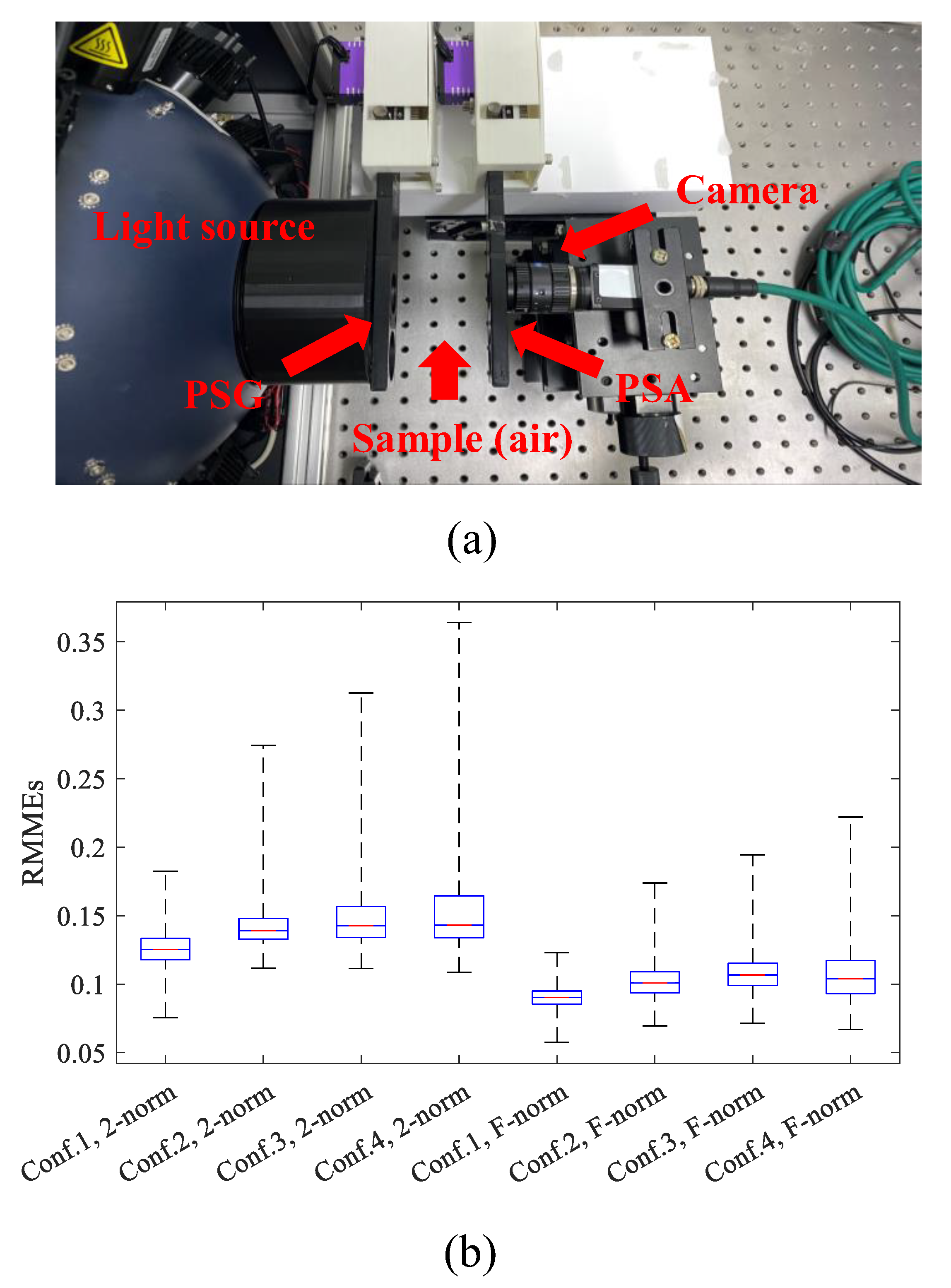
5.2. Effectiveness of the Optimal Criterion: A Practical Experiment

The optimal criterion proposed in Section 4 points out that the optimal orientation angle configuration of polarizers is (c°, c° + 60°, c° + 120°). As a supplement to the simulation experiment, we conducted a simple experiment to verify the effectiveness of the optimal criterion.

In the experiment, images of MMs of air are measured by our 3 × 3 MM imaging system under different orientation angle configurations. We can verify the effectiveness of the optimal criterion via a direct comparison of RMMEs under different configurations. The experiment setup is shown in Figure 5a. The basic architecture of the 3 × 3 MM imaging system is the same as the MM polarimeter shown in Figure 1, where the polarizers are driven by electrical motors, and the light source is an integrating sphere. The system is set to be uncalibrated, of which polarizers in the system are regarded as ideal polarizers in calculations. The orientation angle configurations are set to the optimal one (0°, 60°, 120°), the frequently used ones including (0°, 45°, 90°) and (0°, 45°, 135°), and the random one (0°, 30°, 90°). The resolution of the camera is 2048 × 3072, and the size of the region of interest is 501 × 501, so there are 251,001 MMs in one MM image for comparison. For each orientation angle configuration, we capture one MM image and calculate the RMME for each MM of the image.

Figure 5b shows a boxplot of 2-norm-defined and the F-norm-defined RMMEs for the MMs of air under the four orientation angle configurations, where Conf. 1, Conf. 2, Conf. 3 and Conf. 4 are (0°, 60°, 120°), (0°, 45°, 90°), (0°, 45°, 135°) and (0°, 30°, 90°), respectively. It can be seen in Figure 5b that the RMMEs of the optimal configuration are smaller than the others in terms of the minimum value, the 25th percentile, the 50th percentile, the 75th percentile, and the maximum value. Again, the experimental result is in accord with the theoretical analysis and simulation.

5.3. Three States vs. Four States

As we mentioned before, there are 3 × 3 MM polarimeters that need to measure the intensity of the transmitted light of the sample sixteen times (different combinations of four states of the PSA and the PSG, respectively) to determine the MM of the sample. This subsection will discuss the optimal orientation angle configuration of the MM polarimeter with PSA and PSG with four states (i.e., the four-states-polarimeter, FSP) briefly and compare the performance of the FSP to the polarimeter with PSA and PSG with three states (i.e., the three-states-polarimeter, TSP).

The mathematical model of the FSP can be expressed as

$$A_{\mathrm{PSA}}^{(4\times 3)}{\rm M}{A}_{\mathrm{PSG}}^{(3\times 4)}=I^{(4\times 4)},$$

(25)

where M is the 3 × 3 MM of the sample; $A_{\mathrm{PSA}}^{\left(4\times 3\right)}$, $A_{\mathrm{PSG}}^{\left(3\times 4\right)}$, I^{(4 × 4)} are matrices with size of 4 × 3, 3 × 4, 4 × 4, respectively. The matrices of $A_{\mathrm{PSA}}^{\left(4\times 3\right)}$ and $A_{\mathrm{PSG}}^{\left(3\times 4\right)}$ satisfy

$$\begin{array}{cc}{A}_{\mathrm{PSA}}^{(4\times 3)}=m_{00}\left[\begin{array}{cc}1\hfill & D_{\mathrm{PSA}}^{\mathrm{T}}\left({\theta }_{\mathrm{PSA}}^{\left(1\right)}\right)\hfill \\ 1\hfill & D_{\mathrm{PSA}}^{\mathrm{T}}\left({\theta }_{\mathrm{PSA}}^{\left(2\right)}\right)\hfill \\ 1\hfill & D_{\mathrm{PSA}}^{\mathrm{T}}\left({\theta }_{\mathrm{PSA}}^{\left(3\right)}\right)\hfill \\ 1\hfill & D_{\mathrm{PSA}}^{\mathrm{T}}\left({\theta }_{\mathrm{PSA}}^{\left(4\right)}\right)\hfill \end{array}\right],& A_{\mathrm{PSG}}^{(3\times 4)}=I_{\mathrm{in}}{m}_{00}{\left[\begin{array}{cc}1\hfill & D_{\mathrm{PSG}}^{\mathrm{T}}\left({\theta }_{\mathrm{PSG}}^{\left(1\right)}\right)\hfill \\ 1\hfill & D_{\mathrm{PSG}}^{\mathrm{T}}\left({\theta }_{\mathrm{PSG}}^{\left(2\right)}\right)\hfill \\ 1\hfill & D_{\mathrm{PSG}}^{\mathrm{T}}\left({\theta }_{\mathrm{PSG}}^{\left(3\right)}\right)\hfill \\ 1\hfill & D_{\mathrm{PSG}}^{\mathrm{T}}\left({\theta }_{\mathrm{PSG}}^{\left(4\right)}\right)\hfill \end{array}\right]}^{\mathrm{T}}\end{array},$$

(26)

and I^{(4 × 4)} satisfies

$$I^{(4\times 4)}=\left[\begin{array}{cccc}{I}_{\mathrm{out}}\left({\theta }_{\mathrm{PSA}}^{\left(1\right)},{\theta }_{\mathrm{PSG}}^{\left(1\right)}\right)& I_{\mathrm{out}}\left({\theta }_{\mathrm{PSA}}^{\left(1\right)},{\theta }_{\mathrm{PSG}}^{\left(2\right)}\right)& I_{\mathrm{out}}\left({\theta }_{\mathrm{PSA}}^{\left(1\right)},{\theta }_{\mathrm{PSG}}^{\left(3\right)}\right)& I_{\mathrm{out}}\left({\theta }_{\mathrm{PSA}}^{\left(1\right)},{\theta }_{\mathrm{PSG}}^{\left(4\right)}\right)\\ I_{\mathrm{out}}\left({\theta }_{\mathrm{PSA}}^{\left(2\right)},{\theta }_{\mathrm{PSG}}^{\left(1\right)}\right)& I_{\mathrm{out}}\left({\theta }_{\mathrm{PSA}}^{\left(2\right)},{\theta }_{\mathrm{PSG}}^{\left(2\right)}\right)& I_{\mathrm{out}}\left({\theta }_{\mathrm{PSA}}^{\left(2\right)},{\theta }_{\mathrm{PSG}}^{\left(3\right)}\right)& I_{\mathrm{out}}\left({\theta }_{\mathrm{PSA}}^{\left(2\right)},{\theta }_{\mathrm{PSG}}^{\left(4\right)}\right)\\ I_{\mathrm{out}}\left({\theta }_{\mathrm{PSA}}^{\left(3\right)},{\theta }_{\mathrm{PSG}}^{\left(1\right)}\right)& I_{\mathrm{out}}\left({\theta }_{\mathrm{PSA}}^{\left(3\right)},{\theta }_{\mathrm{PSG}}^{\left(2\right)}\right)& I_{\mathrm{out}}\left({\theta }_{\mathrm{PSA}}^{\left(3\right)},{\theta }_{\mathrm{PSG}}^{\left(3\right)}\right)& I_{\mathrm{out}}\left({\theta }_{\mathrm{PSA}}^{\left(3\right)},{\theta }_{\mathrm{PSG}}^{\left(4\right)}\right)\\ I_{\mathrm{out}}\left({\theta }_{\mathrm{PSA}}^{\left(4\right)},{\theta }_{\mathrm{PSG}}^{\left(1\right)}\right)& I_{\mathrm{out}}\left({\theta }_{\mathrm{PSA}}^{\left(4\right)},{\theta }_{\mathrm{PSG}}^{\left(2\right)}\right)& I_{\mathrm{out}}\left({\theta }_{\mathrm{PSA}}^{\left(4\right)},{\theta }_{\mathrm{PSG}}^{\left(3\right)}\right)& I_{\mathrm{out}}\left({\theta }_{\mathrm{PSA}}^{\left(4\right)},{\theta }_{\mathrm{PSG}}^{\left(4\right)}\right)\end{array}\right],$$

(27)

where m₀₀ is the average intensity coefficient of the PSA and the PSG; I_in is the intensity of the light source; ${\theta }_{\mathrm{PSA}}^{\left(1\right)}$, ${\theta }_{\mathrm{PSA}}^{\left(2\right)}$, ${\theta }_{\mathrm{PSA}}^{\left(3\right)}$, ${\theta }_{\mathrm{PSA}}^{\left(4\right)}$ and ${\theta }_{\mathrm{PSG}}^{\left(1\right)}$, ${\theta }_{\mathrm{PSG}}^{\left(2\right)}$, ${\theta }_{\mathrm{PSG}}^{\left(3\right)}$, ${\theta }_{\mathrm{PSG}}^{\left(4\right)}$ are four orientation angles of the PSA and the PSG, respectively; D_PSA(θ_PSA) and D_PSG(θ_PSG) are diattenuation vectors of the PSA and the PSG with orientation angle of θ_PSA and θ_PSG, respectively; I_out (${\theta }_{\mathrm{PSA}}^{\left(i\right)}$_, ${\theta }_{\mathrm{PSG}}^{\left(j\right)}$) is the intensity of the transmitted light of the sample under the PSA angle of ${\theta }_{\mathrm{PSA}}^{\left(i\right)}$ and the PSG angle of ${\theta }_{\mathrm{PSG}}^{\left(j\right)}$.

According to Equation (25), the measured MM of the sample, denoted by $\widehat{M}$, can be expressed as

$$\widehat{M}={\left[A_{\mathrm{PSA}}^{(4\times 3)}\right]}^{+}{I}^{(4\times 4)}{\left[A_{\mathrm{PSG}}^{(3\times 4)}\right]}^{+},$$

(28)

where [${\mathbf{A}}_{\mathrm{PSA}}^{\left(4\times 3\right)}$]⁺ and [${\mathbf{A}}_{\mathrm{PSG}}^{\left(3\times 4\right)}$]⁺ are Moore-Penrose generalized inverse matrices of ${\mathbf{A}}_{\mathrm{PSA}}^{\left(4\times 3\right)}$ and ${\mathbf{A}}_{\mathrm{PSG}}^{\left(3\times 4\right)}$, respectively. If there is not any instrumental error, and ${\mathbf{A}}_{\mathrm{PSA}}^{\left(4\times 3\right)}$ and ${\mathbf{A}}_{\mathrm{PSG}}^{\left(3\times 4\right)}$ are full column rank and full row rank, respectively, then $\widehat{M}$ will equal to M. Conversely, if there are instrumental errors so that Equation (25) is over-determined, $\widehat{M}$ is a least squares solution with minimum norm.

There is a work [23] points out that 2-norm-defined condition numbers of ${\mathbf{A}}_{\mathrm{PSA}}^{\left(4\times 3\right)}$ and ${\mathbf{A}}_{\mathrm{PSG}}^{\left(4\times 3\right)}$ are minimized by an orientation angle configuration that is (0°, 45°, 90°, 135°). Moreover, according to our analysis, the F-norm-defined condition numbers of ${\mathbf{A}}_{\mathrm{PSA}}^{\left(4\times 3\right)}$ and ${\mathbf{A}}_{\mathrm{PSG}}^{\left(4\times 3\right)}$ are also minimized by such an orientation angle configuration. A coincidence is that the minimized condition numbers of ${\mathbf{A}}_{\mathrm{PSA}}^{\left(4\times 3\right)}$ and ${\mathbf{A}}_{\mathrm{PSG}}^{\left(4\times 3\right)}$ are fully the same as the minimized condition numbers of A_PSA and A_PSG. That implies error resistances of the FSP and the TSP are the same under the frame of the perturbation analysis [23].

To compare the performances of the TSP and the FSP, we conducted a supplemental simulation. The simulation is similar to one introduced in Section 5.1, where instrumental errors were added into the orientation angle, the diattenuations and the intensities measured by the camera for both the schemes, and RMMEs defined by the 2-norm and the F-norm are calculated. Angle errors and intensity errors were added to the four angles and the sixteen intensities for the FSP. The statistical distributions of random errors in the FSP and the TSP are the same. In the simulation, the FSP and the TSP are optimized, where the diattenuation of the PSAs and the PSGs equal one, and orientation angle configurations are optimal.

A boxplot of RMMEs of 5000 times of simulation is shown in Figure 6, where the maximum values of RMMEs of different polarimeters and different norms are outliers, which are marked by “+”. It can be seen from Figure 6 that, for both the 2-norm and the F-norm, the RMME of FSP is always lower than that of TSP in terms of the minimum value, the 25th percentile, the 50th percentile, the 75th percentile, the upper adjacent value, and even the abnormal maximum value. Therefore, the error resistance of FSP is better than that of TSP significantly. This conclusion is reasonable since the TSP needs more time for measurement. In fact, in 4 × 4 MM polarimetry, an effective way to improve the accuracy of measurement is to increase the number of measurements, such as dual-rotating retarder MM polarimeter [16,19]. However, the cost of time and the accuracy need to be balanced. Therefore, how to reach a high accuracy as much as possible at the minimum times of measurements is still a valuable problem.

6. Conclusions

In this paper, based on the rigorous mathematical analysis, an optimal criterion of the designation of polarizers in a canonical 3 × 3 Mueller matrix polarimeter is given. The mathematical analysis reveals the fact that the polarimeter with the optimal orientation angle configurations (0°, 60°, and 120°) of polarizers has a robust optimal error resistance, which inherently ensures a minimal relative measurement error statistically. Moreover, to ensure the effectiveness of the mathematical analysis, a simulation is conducted. The simulation experiment shows that the mathematical analysis is effective, and the average relative error reaches a minimal value under the optimal orientation angle configuration. In contrast to the frequently used orientation angle configuration, the RMME reduced by up to 32% under the condition of our simulation experiment when the optimal design criterion was adopted.

References

1. Wang, Y.; Wang, J.; Meng, J. Detection of non-small cell lung cancer cells based on microfluidic polarization microscopic image analysis. Electrophoresis 2019, 40, 1202–1211. [Google Scholar] [CrossRef] [PubMed]
2. Liu, W.; Xiong, J.; Liu, J. Polarization multi-parametric imaging method for the inspection of cervix cell. Opt. Commun. 2021, 488, 126846. [Google Scholar] [CrossRef]
3. He, C.; Chang, J.; Salter, P.S. Revealing complex optical phenomena through vectorial metrics. Adv. Photonics 2022, 4, 026001. [Google Scholar] [CrossRef]
4. Dong, Y.; Wan, J.; Si, L. Deriving polarimetry feature parameters to characterize microstructural features in histological sections of breast tissues. IEEE Trans. Bio. Med. Eng. 2020, 68, 881–892. [Google Scholar] [CrossRef]
5. Ahmad, I.; Khaliq, A.; Iqbal, M. Mueller matrix polarimetry for characterization of skin tissue samples: A review. Photodiagnosis Photodyn. Ther. 2020, 30, 101708. [Google Scholar] [CrossRef]
6. Ghosh, N.; Vitkin, I.A. Tissue polarimetry: Concepts, challenges, applications, and outlook. J. Biomed. Opt. 2011, 16, 110801. [Google Scholar] [CrossRef]
7. Li, Y.; Zhang, S.; Wu, L. Polarization microwave-induced thermoacoustic imaging for quantitative characterization of deep biological tissue microstructures. Photonics Res. 2022, 10, 1297–1306. [Google Scholar] [CrossRef]
8. Barnes, B.M.; Goasmat, F.; Sohn, M.Y. Enhancing 9 nm node dense patterned defect optical inspection using polarization, angle, and focus. Proc. SPIE 2013, 8681, 134–141. [Google Scholar]
9. Kazama, A.; Oshige, T. A defect inspection technique using polarized images for steel strip surface. Proc. SPIE 2008, 7072, 153–161. [Google Scholar]
10. Lu, S.Y.; Chipman, R.A. Interpretation of Mueller matrices based on polar decomposition. JOSA A 1996, 13, 1106–1113. [Google Scholar] [CrossRef]
11. Swami, M.K.; Manhas, S.; Buddhiwant, P. Polar decomposition of 3 × 3 Mueller matrix: A tool for quantitative tissue polarimetry. Opt. Express 2006, 14, 9324–9337. [Google Scholar] [CrossRef] [PubMed]
12. Qi, J.; Ye, M.; Singh, M. Narrow band 3×3 Mueller polarimetric endoscopy. Biomed. Opt. Express 2013, 4, 2433–2449. [Google Scholar] [CrossRef] [PubMed]
13. Fu, Y.; Huang, Z.; He, H. Flexible 3 × 3 Mueller matrix endoscope prototype for cancer detection. IEEE Trans. Instrum. Meas. 2018, 67, 1700–1712. [Google Scholar] [CrossRef]
14. Tyo, J.S. Design of optimal polarimeters: Maximization of signal-to-noise ratio and minimization of systematic error. Appl. Opt. 2002, 41, 619–630. [Google Scholar] [CrossRef]
15. Twietmeyer, K.M. Mueller matrix retinal imager with optimized polarization conditions. Opt. Express 2008, 16, 21339–21354. [Google Scholar] [CrossRef]
16. Ambirajan, A.; Lock, D.C., Jr. Optimum angles for a Mueller matrix polarimeter. Proc. SPIE 1994, 2265, 314–326. [Google Scholar]
17. Qi, J.; Elson, D.S.; Stoyanov, D. Eigenvalue calibration method for 3 × 3 Mueller polarimeters. Opt. Lett. 2019, 44, 2362–2365. [Google Scholar] [CrossRef]
18. Ramella-Roman, J.C.; Duncan, D.D. A new approach to Mueller matrix reconstruction of skin cancer lesions using a dual rotating retarder polarimeter. Proc. SPIE 2006, 6080, 107–113. [Google Scholar]
19. Goldstein, D.H. Mueller matrix dual-rotating retarder polarimeter. Appl. Opt. 1992, 31, 6676–6683. [Google Scholar] [CrossRef]
20. Huang, S.X.; Wu, G.B.; Chan, K.F. Demonstration of a terahertz multi-spectral 3 × 3 Mueller matrix polarimetry system for 2D and 3D imaging. Opt. Express 2021, 29, 14853–14867. [Google Scholar] [CrossRef]
21. Del Hoyo, J.; Sanchez-Brea, L.M.; Gomez-Pedrero, J.A. High precision calibration method for a four-axis Mueller matrix polarimeter. Opt. Lasers Eng. 2020, 132, 106112. [Google Scholar] [CrossRef]
22. Bueno, J.M. Polarimetry using liquid-crystal variable retarders: Theory and calibration. J. Opt. A Pure Appl. Op. 2000, 2, 216. [Google Scholar] [CrossRef]
23. Qi, J. Development of Optical Polarisation Resolved Endoscopy. Ph.D. Thesis, Imperial College London, London, UK, 2014. [Google Scholar]
Figure 1. Diagram of a canonical 3 × 3 MM imaging polarimeter.
Photonics 10 01087 g001
Figure 2. (a) Mesh surface plot of the two-dimensional distribution of cond 2 1 (APSA) under DPSA = 1 and different (x, y); (b) one-dimensional distributions of cond2(APSA) from x = 58° to x = 62° under DPSA = 1 and different y.
Photonics 10 01087 g002
Figure 3. Two-dimensional distributions of average RMMEs and corresponding average upper boundaries with respect to different orientation angle configurations of the MM polarimeter: (a) 2-norm-defined distributions for air; (b) F-norm-defined distributions for air; (c) 2-norm-defined distributions for QWP; (d) F-norm-defined distributions for QWP.
Photonics 10 01087 g003
Figure 4. Average RMMEs and corresponding average upper boundaries of different angle configurations: (a) 2-norm-defined and F-norm-defined RMMEs; (b) 2-norm-defined and F-norm-defined upper boundaries.
Photonics 10 01087 g004
Figure 5. (a) The 3 × 3 MM imaging system; (b) Boxplot of 2-norm-defined and the F-norm-defined RMMEs for the MMs of air under four orientation angle configurations.
Photonics 10 01087 g005
Figure 6. Boxplot of 2-norm-defined and F-norm-defined RMMEs of TSP and FSP. The maximum values of RMMEs are marked by “+”.
Photonics 10 01087 g006