A New Machine Learning Algorithm to Simulate the Outlet Flow in a Reservoir, Based on a Water Balance Model

Abstract

Predicting water losses and final storage in reservoirs has become increasingly relevant in the efficient control and optimization of water provided to agriculture, livestock, industry, and domestic consumption, aiming to mitigate the risks associated with flash floods and water crises. This research aims to develop a new Machine Learning (ML) algorithm based on a water balance model to simulate the outflow in the Cuchoquesera reservoir in the Ayacucho region. The method uses TensorFlow (TF), a powerful interface for graphing and time series forecasting, for data analysis of hydrometeorological parameters (HMP), inflow (QE_obs), and outflow (QS_obs) of the reservoir. The ML water balance model is fed, trained, and calibrated with daily HMP, QE_obs, and QS_obs data from the Sunilla station. The results provide monthly forecasts of the simulated outflow (QS_sim), which are validated with QS_obs values, with significant validation indicators: NSE (0.87), NSE-Ln (0.83), Pearson (0.94), R² (0.87), RMSE (0.24), Bias (0.99), RVB (0.01), NPE (0.01), and PBIAS (0.14), with QS_obs being slightly higher than QS_sim. Therefore, it is important to highlight that water losses due to evaporation and infiltration increased significantly between 2019 and 2023.

1. Introduction

Water is an indispensable resource for life and sustainable development; its scarcity can have dramatic consequences, including the loss of human life and impacts on urban, agricultural, livestock, and industrial sectors [1]. However, only 2.5 to 3% of the Earth’s freshwater is accessible, and a little more than 1.2% is found on the surface [2]. For this reason, water infrastructure—such as reservoirs and dams—is essential for supplying water to the population, as well as providing water during extreme events such as droughts and seasonal floods [3,4,5,6].

Also, the use of reservoirs formed behind dams allows the generation of hydroelectric power, which is a renewable energy source that contributes to the reduction of carbon emissions and the mitigation of the energy deficit, although it can also have negative environmental impacts, such as disrupting aquatic–terrestrial ecosystems and creating barriers to the movements and exchange of organisms between habitats [7,8,9].

Water entering a reservoir is subject to various losses due to evaporation, infiltration, and sedimentation, making it difficult to determine the amount of water available [10]. This issue requires advanced approaches, such as the development of water balance models using ML techniques, which allow adaptation to dynamic scenarios and improve decision-making in real time [2,3,4].

On the other hand, the problem of water management becomes highly relevant in some arid regions such as Qatar, where rainfall is scarce. A combination of water balance with Monte Carlo simulations allows a significant estimate of aquifer recharge, amounting to 58.7 m³/year, which is essential for sustainable management to preserve groundwater in times of high climatic variability [11].

Another key scenario for water balance is marine–coastal ecosystems, where vertical and horizontal water exchanges can be measured. The authors of [12] conducted a study in Lake Gardno (Poland) between 2003 and 2007, and found that 10% of the water originated from the Baltic Sea, while 86% was attributed to terrestrial inputs from rivers and precipitation (Pp). These results underline the importance of quantifying external sources in water management during the development of a water balance in marine ecosystems, especially in the estimation of water losses due to saline intrusion and climate variability.

Another scenario where water balances are critical for predicting water availability is in melt-dependent zones such as glacial environments in the Cordillera Blanca, Peru. This was confirmed by [13], who performed a mass and energy balance model in the Shallap Glacier between 2006 and 2008, based on meteorological data and in situ validations with 20 stakes around melt zones. The results showed a loss of −0.32 ± 0.4 mwe (meter water equivalent) between 2006 and 2007, followed by a net gain of 0.51 ± 0.56 mwe. In areas above 5000 masl, the loss was −0.33 mwe due to snow accumulation. In contrast, in lower areas, the loss reached 1.97 ± 0.68 mwe between both years, due to the reduction of solid precipitation and the increase in temperatures. This phenomenon reduces surface albedo, accelerates melting, and displaces the snow line, which threatens the water supply of the Andean population [14].

In the Ayacucho region of Peru, the high Andean areas face significant water challenges due to the retreat of glaciers, which reduces natural water storage and triggers recurrent droughts and seasonal floods, driven by the region’s climatic diversity and the influence of El Niño–Southern Oscillation (ENSO) [15,16,17]. Similarly, the Apacheta microwatershed (headwaters of the Cachi basin and a critical groundwater recharge zone) is suffering the impacts of climate change, affecting water supply to the primary intake, where headwater tributaries are diverted. Water is then conveyed to the Cuchoquesera reservoir in the Chuschi district, Cangallo province of Ayacucho, with a storage capacity of 80 million m³, which supplies 20% of the region’s population and 60% of local farmers [18,19].

In this sense, the Cuchoquesera reservoir plays a key role in mitigating shortages and ensuring water supply for agricultural, livestock, and industrial activities [20,21]. This justifies the need to measure water availability and losses by developing a water balance model with ML techniques, such as the study by [3] at the Sikirit reservoir, Thailand. The implementation of a water balance model requires input data on precipitation (Pp), evaporation (Ev), relative humidity (RH), and ambient temperature (Tamb) recorded at the Sunilla station, and inflow (QE_obs) and outflow (QS_obs) observed or measured in the Cuchoquesera reservoir. This enables optimized water allocation while accounting for evaporation losses, infiltration, and drought stress in dry periods [22,23].

The hydrological cycle in the wetland ecosystems of the Apacheta microwatershed plays an essential role in surface, subsurface, and groundwater recharge for water supply to the Cuchoquesera reservoir [24]. This micro-watershed is not immune to the effects of climate change, as indicated by [25], who confirmed a significant increase in surface soil temperature (SST), alongside significant reductions in snowpack and vegetation cover, which directly influences evapotranspiration (ET), infiltration, and surface and subsurface runoff, ultimately altering the water yield delivered to the Cuchoquesera reservoir. These variations in the hydrological cycle require the development of a water balance model using ML techniques, adaptable to variations in precipitation (Pp), prolonged droughts, and non-stationary hydrometeorological parameters (HMP) modified by extreme events [26,27].

The main challenge of this research lies in developing an ML algorithm that overcomes the limitations of conventional methods, integrating multivariate data (Pp, Ev, RH, Tamb, QE_obs) with inherent uncertainty and practical requirements (speed, interpretability, scalability), to simulate the outflow (QS_sim) and predict its behavior more accurately [27,28,29,30]. The ML water balance model will be trained with a subset of hydrometeorological data from the Sunilla station and the Cuchoquesera reservoir, and the results will be validated with QE_obs and QS_obs data measured in the Cuchoquesera reservoir. From these results, the storage volume of the reservoir will be calculated, and monthly water losses from evaporation and infiltration will be estimated [31].

Hydrometeorological data from the Sunilla station were provided by the Operations and Maintenance Office (OPEMAN) of the Regional Government of Ayacucho (GRA), with records from 2013 to 2023, and the QE_obs data were obtained from the records of the limnimeter installed in the Cuchoquesera reservoir. The QS_obs were obtained from the records located in the control room of the dam, which feed the water balance model with TensorFlow (TF) based on ML and Long Short-Term Memory (LSTM) for analyzing fluctuations in QS_sim in the time trend series, with estimates that exceed the physical models (NSE > 0.8) in flow prediction with limited data [32,33].

In this sense, the proposal of a new ML algorithm based on the physical fundamentals of water balance to simulate the reservoir outflow is developed using a multilayer Perceptron Neural Network (MLP), with one hidden layer (1000 neurons), Sigmoid activation, and TF LSTM integration [34]. The code is built using the Python 3.10 programming language, which uses libraries integrated with artificial neural networks (ANNs) for training (2013–2021) and testing (2022–2023) on monthly partitioned data. The validation of the simulated data is performed with indicators including the Nash–Sutcliffe Efficiency (NSE) coefficient, Nash–Sutcliffe-Ln (NSE-Ln) coefficient, Pearson correlation coefficient, coefficient of determination (R²), and Root Mean Squared Error (RMSE), among others [35,36].

Considering the impact of the Cuchoquesera reservoir within the Cachi watershed, we set out to build a water balance model using a new ML algorithm to simulate the outflow of the reservoir, taking advantage of innovative LSTM techniques with TF. The success of the results achieved in this research will allow us to make a temporal projection of the behavior of QS_sim and anticipate the water losses of the reservoir. This will provide a scientific basis necessary to address potential future scenarios of water scarcity in the region influenced by the Cuchoquesera reservoir.

2. Materials and Methods

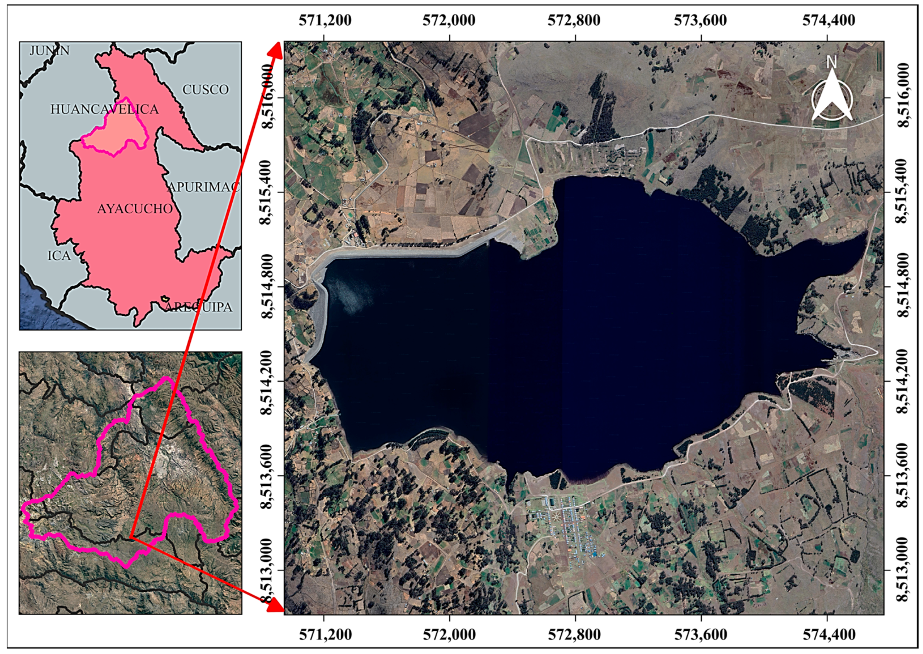
2.1. Study Area

Geographically, the Cuchoquesera dam is located in the population centers of Cuchoquesera and Pampamarca in the district of Chuschi, province of Cangallo, department of Ayacucho, within the Mantaro river basin, at an elevation of 3730 m above sea level, as shown in Figure 1. The reservoir receives water via a diversion channel from the Churiac stream and at its primary intake from the Apacheta, Choccoro, and Chicllarazo rivers. This inflow is conveyed through a return-flow channel into the Cuchoquesera reservoir and is then distributed to the towns and population of Huamanga for domestic, agricultural, livestock, and industrial uses.

The Cuchoquesera dam was completed in 2002 and became operational in the same year. Currently, the Regional Government of Ayacucho, through the Sub-management of Works and the Operations and Maintenance Office (OPEMAN, by its Spanish acronym), is in charge of the maintenance and stability of the dam. The Cuchoquesera reservoir has a storage capacity of 80 million cubic meters (MCMs). The dam is of concrete type, i.e., conventional, with a maximum height of 42.0 m and a crest length of 390.72 m [19,37].

Table 1. Characteristics of the Cuchoquesera reservoir.

Article	Description
Function	Water storage and supply managed by the Regional Government of Ayacucho, through the Sub-management of Works and the Operations and Maintenance Office (OPEMAN), for treatment and distribution of water for domestic and agricultural uses.
Altitude	3730 m above sea level
Total Capacity	80 million cubic meters
Water Use	18 million cubic meters for drinking water and 42 million cubic meters for agriculture
Dam Structure	42 m structural height and crest length of 390.72 m
Bottom outlet (main)	Capacity: 32 m3/s
Bottom outlet (auxiliary)	Capacity: 1–8.6 m3/s
Spillway capacity	Crest length: 247.70 m Discharge capacity: 9.32 m3/s

shows the characteristics of the Cuchoquesera reservoir.

2.2. Database

For the development of the water balance simulation model, it is first necessary to request access to HMP data recorded by the OPEMAN of the Regional Government of Ayacucho. The following steps should be followed:

• Compile the records from the HMP sheets of the Sunilla meteorological station, the inflow and outflow data, and the structural profile of the Cuchoquesera dam.
• Collect the historical data of the Sunilla station HMP: precipitation (Pp), evaporation (Ev), relative humidity (RH), and ambient temperature (Tamb).
• Obtain inflow (QE_obs) and outflow (QS_obs) data for the reservoir.

A minimum of eleven years of historical data is required to calibrate the Cuchoquesera reservoir water balance simulation model. The data used include Pp, Ev, RH, Tamb, QE_obs, and QS_obs.

2.3. Data Analysis

Table 2. Descriptive statistics of hydrometeorological parameters and observed flows.

Parameter	Mean	Std	Min	25%	50%	75%	Max
Pp (mm)	65.06	68.50	0.00	9.00	41.97	109.10	293.70
Ev (mm)	68.39	60.40	0.00	0.00	89.30	107.10	306.90
RH (%)	79.92	17.72	0.00	78.31	81.53	85.01	100.00
Tamb (°C)	9.24	3.72	0.00	8.38	9.80	11.10	17.36
QE_obs (m3/s)	2.30	2.71	0.01	0.29	1.00	3.57	9.89
QS_obs (m3/s)	2.40	1.65	0.01	0.69	2.67	3.96	4.93

Data provided by OPEMAN-GRA.

shows the monthly HMP data recorded at the Sunilla meteorological station and the Cuchoquesera reservoir, during the period from 2013 to 2023, which includes 132 records of Pp, Ev, RH, Tamb, QE_obs, and QS_obs, respectively. Pp showed a mean value of 65.06 mm/month, with outliers reaching up to 293.70 mm/month, possibly linked to ENSO according to 4,35]. On the other hand, Ev showed a mean value of 60.40 mm/month, which suggests the presence of prolonged periods of low Ev, potentially reflecting extreme dry periods with a minimum of 0% RH, which is unlikely under normal climatological conditions. Given that the mean value of RH is 79.24%, this suggests either possible errors in the measurement sensors or unexplained extreme conditions. The mean value of Tamb is 9.24 °C, with a standard deviation of 3.72 °C, reflecting seasonal variability as will be shown below. The mean value of QE_obs is 2.3 m³/s with a variability of standard deviation $\sigma =2.71 {\mathrm{m}}^3/\mathrm{s}$, and the mean value of QS_obs is 2.4 m³/s with $\sigma =1.65 {\mathrm{m}}^3/\mathrm{s}$, reflecting the influence of precipitation and controlled retained management. In addition, it should be mentioned that the data were validated with barometric measurements, which reinforces their reliability.

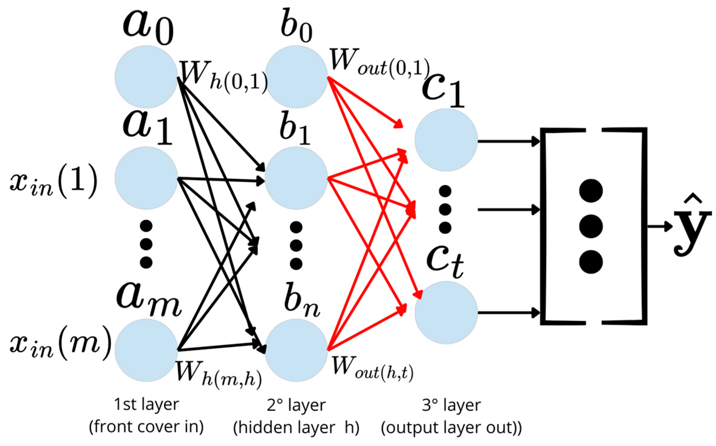
2.4. Artificial Neural Network (ANN)

ANNs are inspired by the structure and functioning of biological neurons, where information is transmitted through interconnected connections to process stimuli and responses. Similarly, ANNs process complex data by means of computational algorithms, allowing modeling nonlinear relationships and performing prediction or classification tasks, being able to approximate real-valued, discrete, or vector functions, through several training layers to be more efficient [38,39]. With each connection, the input from the cell to other cells is accumulated, along with the external threshold, resulting in the output signal. In other words, the sum of the weighted inputs, the weight of the neurons w and bias b, will produce the net value, Y.

The type of neural network for this research work is an MLP. Figure 2 shows how the input layer is connected to the hidden layers, and then to the output layer, enabling forward propagation [40], following three simple steps:

• The input layer propagates forward to generate the network’s output.

$$z=w_0{x}_0+w_1{x}_1+\dots +w_n{x}_n=\sum _{j=0}^n{x}_j{w}_j=w^{T}x$$

(1)

2.

The error between the predicted and actual output is computed by means of a cost function.

$$J\left(w\right)=-\sum _{i=1}^n{y}^i\mathit{log}\left(a^{\left(i\right)}\right)+\left(1-y^{\left(i\right)}\right)\mathit{log}(1-a^{\left(i\right)})+L2$$

(2)

3.

The error is backpropagated through the network, computing the derivatives with respect to the weights, and the model is updated accordingly. This process is repeated iteratively.

2.5. TensorFlow (TF)

The TF is a versatile interface that facilitates the implementation and execution of complex ML algorithms. It was developed and used by Google, which later, in 2015, released it as open-source software under the permissive Apache 2.0 license. It can run on both CPUs and GPUs, with the latter offering superior performance, enabled by CUDA technology, particularly when processing large datasets [41,42].

For the modeling of the data analysis through time series of the HMP with the use of the TensorFlow framework and the LSTM model, the physical basis of the water balance is applied. The new algorithm with ML is implemented in Python code, using input data from the Sunilla meteorological station and the Cuchoquesera reservoir. Subsequently, the model is trained to predict possible future scenarios related to the climatic or hydrological behavior of the reservoir under study [33,43,44].

2.6. Long Short-Term Memory (LSTM)

The LSTM is a deep learning algorithm, designed to learn and process sequential data, primarily for regression tasks, to develop predictions with time series data and simultaneously address long-term dependencies by selectively forgetting irrelevant information and retaining important data [45,46]. This allows for observing the behavior of HMP and learning from the input values, observing fluctuations over time, both in training and testing, as well as developing a forecast of the behavior of these parameters over time.

3. Water Balance Model and Simulation

The water balance equation describes how water received by a system through precipitation is subsequently distributed, including its partitioning into evapotranspiration, runoff, and infiltration. This method is based on the principle of conservation of mass, which states that water is neither created nor destroyed, but only transformed. Using this equation, the different quantities of water participating in the hydrological cycle can be related [47].

For the implementation of the new algorithm with ML, a one-layer artificial neural network is used, following the detailed structure as shown in Figure 3. To start building the code, the required packages are imported: Numpy 1.22.4 (mathematical operations), Pandas 2.2.2 (data manipulation), Matplotlib 3.7.1 (generate graphs), and Scikit-Learn 1.2.2 (learning library for predictive analytics). Subsequently, the input data $x_i=[Pp, Ev, Tamb, RH, QE-obs]$ and the output data $y=[QS\_obs]$ are imported in CSV format. Assigning a random_state = 500 for the division of the input data, the data are divided into 80% for training and 20% for the model validation test. After this, we proceed with the construction of the model using Algorithm 1 (Appendix A), assigning the following features:

• Hidden_layer_sizes (500,) asks to create a hidden layer of 500 neurons, for which each input will check Equation (3).
• Activation = ‘logistic’ is used to avoid linearity and model the input data, allowing it to learn the model according to Equation (4).
• Max_iter = 10,000 is the maximum number of iterations until the model converges.
• Random state = 50 is a pseudo-random number generator to initialize the weights and biases of the ANN.

Subsequently, the model is trained using model.fit(x_train, y_train), performing the stages of propagation, error calculation, and backpropagation, with a maximum of 10,000 iterations, until the error is reduced. When calling model.predict(x), the predictions are made; this involves calculating the weighted sum plus biases, and through the activation function, it transforms the input data into the output data, which allows generating final predictions of the model, which will be validated by calculating the mean square error (MSE).

Network input equation:

$$z=\left(w_1·Pp\right)+\left(w_2·Ev\right)+\left(w_3·RH\right)+\left(w_4·Tamb\right)+\left(w_5·QE\_obs\right)+b$$

(3)

Equation of the activation function:

$$\sigma \left(z\right)={\displaystyle \frac{1}{1+e^{\left\{-z\right\}} }}$$

(4)

To estimate the water losses in the Cuchoquesera reservoir based on the results of the simulated flow, it is defined with the following equation:

$$\pm L=Pp-Ev+\left(QE\_obs\right)-\left(QS\_obs\right)-S_i+S_s$$

(5)

where $S_i$ is the initial storage at a given time; $S_s$ is the final storage at a given time; $L$ is the water loss as a function of the initial and final storage states at a given time; QE_obs is the inflow to the reservoir; and QS_obs is the outflow from the reservoir.

In Equation (5), if the value of $L$ is negative, it means that the reservoir is losing water through evaporation and infiltration or other external factors; conversely, it means that there is more water entering the reservoir than leaving it, indicating greater accumulation.

If the value of $L=0$, then Equation (5) satisfies the principle of conservation of mass, where the amount of water entering the reservoir is equal to the amount of mass leaving it, so we have a water balance expression (Equation (6)) as a function of HMP and inflow and outflow:

$$Pp+\left(QE\_obs\right)+S_s=Ev+\left(QS\_obs\right)+S_i$$

(6)

4. Results

4.1. Time Series Projections of HMPs with TF

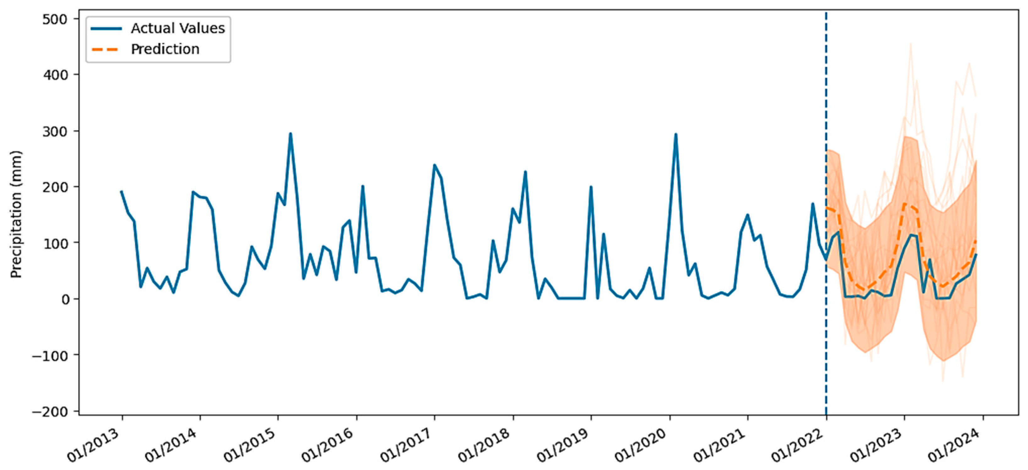
4.1.1. Precipitation (Pp)

Monthly precipitation data were obtained from the accumulation of daily data for each month during the period 2013 to 2023. Figure 4 illustrates the historical variability and the predicted monthly cumulative Pp at Cuchoquesera reservoir. The graph contains two series of data: the blue line represents the real variability of the Pp in the study years, showing higher Pp levels in the first months (January–March), months with little Pp in the middle of the year (June to September), and finally an increase again in the later months (October to December), repeating the cycle. The orange line indicates the prediction interval from January 2022 to December 2024, reflecting the same pattern as the observed Pp. The shaded area, representing a 95% confidence interval, suggests a moderate degree of uncertainty, especially during high Pp peaks, which is consistent with the variable nature of weather events and captures relevant trends.

Figure 5 illustrates the seasonal variation of the monthly mean Pp, highlighting recurring patterns observed during the study period. The months with the highest Pp levels are from January to April, and the months from June to September reflect the lowest Pp levels. The orange shaded band around the main line indicates the monthly variability and confidence intervals, showing greater certainty in the months with less rainfall.

The relationship between observed inflow (QE_obs) and observed outflow (QS_obs) to precipitation (Pp) in Figure 6 shows that QE_obs is proportional to Pp, i.e., the higher the Pp, the higher the inflow to the reservoir, while the lower the Pp, the lower the QE_obs. On the other hand, QS_obs is inversely proportional to Pp, since, under conditions of abundant rainfall, QS_obs will be lower, whereas if Pp is low, QS_obs will be higher. This occurs because at the beginning of each month, the Cuchoquesera reservoir is filled to 80 MCMs, and at that time, the reservoir outflow is controlled only for population consumption; in months when the amount of rainfall reaches the total level of the reservoir, the water resource is distributed for agricultural and population consumption, which demands more water outflow from the Cuchoquesera reservoir.

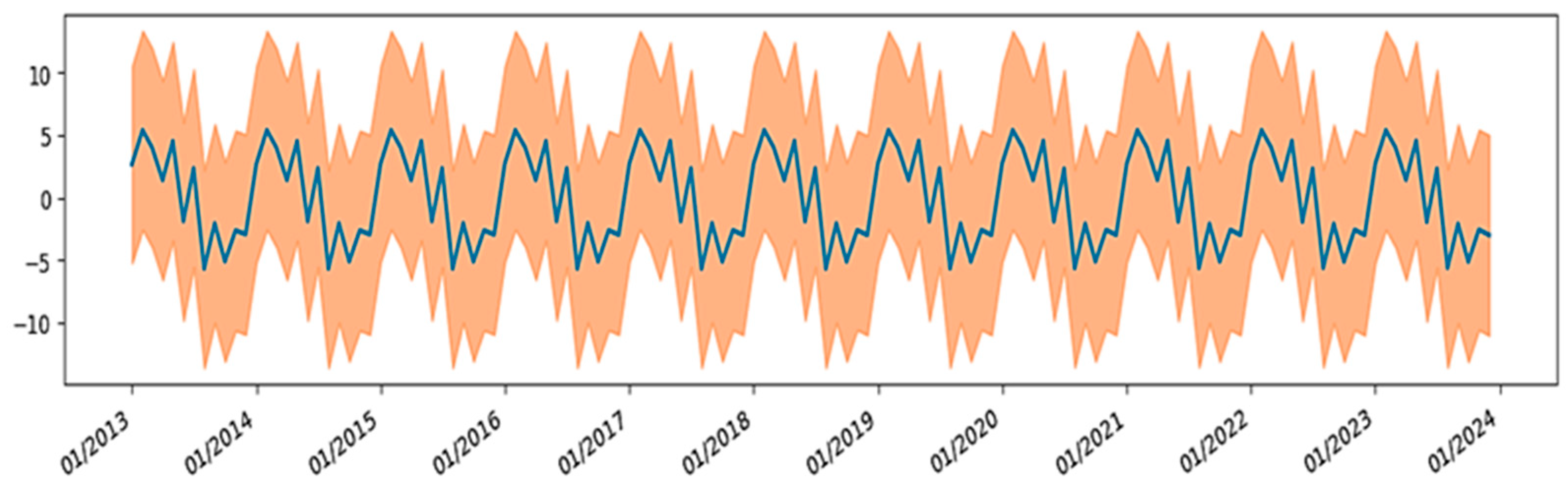
4.1.2. Evaporation (Ev)

Monthly evaporation data were obtained by accumulating daily data for the period 2013–2023. Figure 7 illustrates the historical variability and the predicted monthly accumulated Ev in the Cuchoquesera reservoir. High peaks of Ev are observed between January 2013 and March 2016, reaching a maximum value of 300 mm in 2015, while the minimum value of 0 mm occurs between March and December 2020. Subsequently, Ev stabilizes around 100 mm from 2021 to March 2023, decreasing to 0 mm for the remaining period. The forecast line maintains a stable pattern around 100 mm, with some high peaks of 120 mm between January and March each year. The shaded area represents a 95% confidence interval, with a notable amplitude indicating the range of possible variations in the prediction.

Figure 8 illustrates the Ev seasonal variation, highlighting the recurrent patterns observed during the study period. The months with the highest amount of water Ev are observed between January and April, showing higher peaks, and the months from May to November reflect lower Ev levels. The orange band in the graph represents a 95% confidence interval, being more pronounced in months with lower variability.

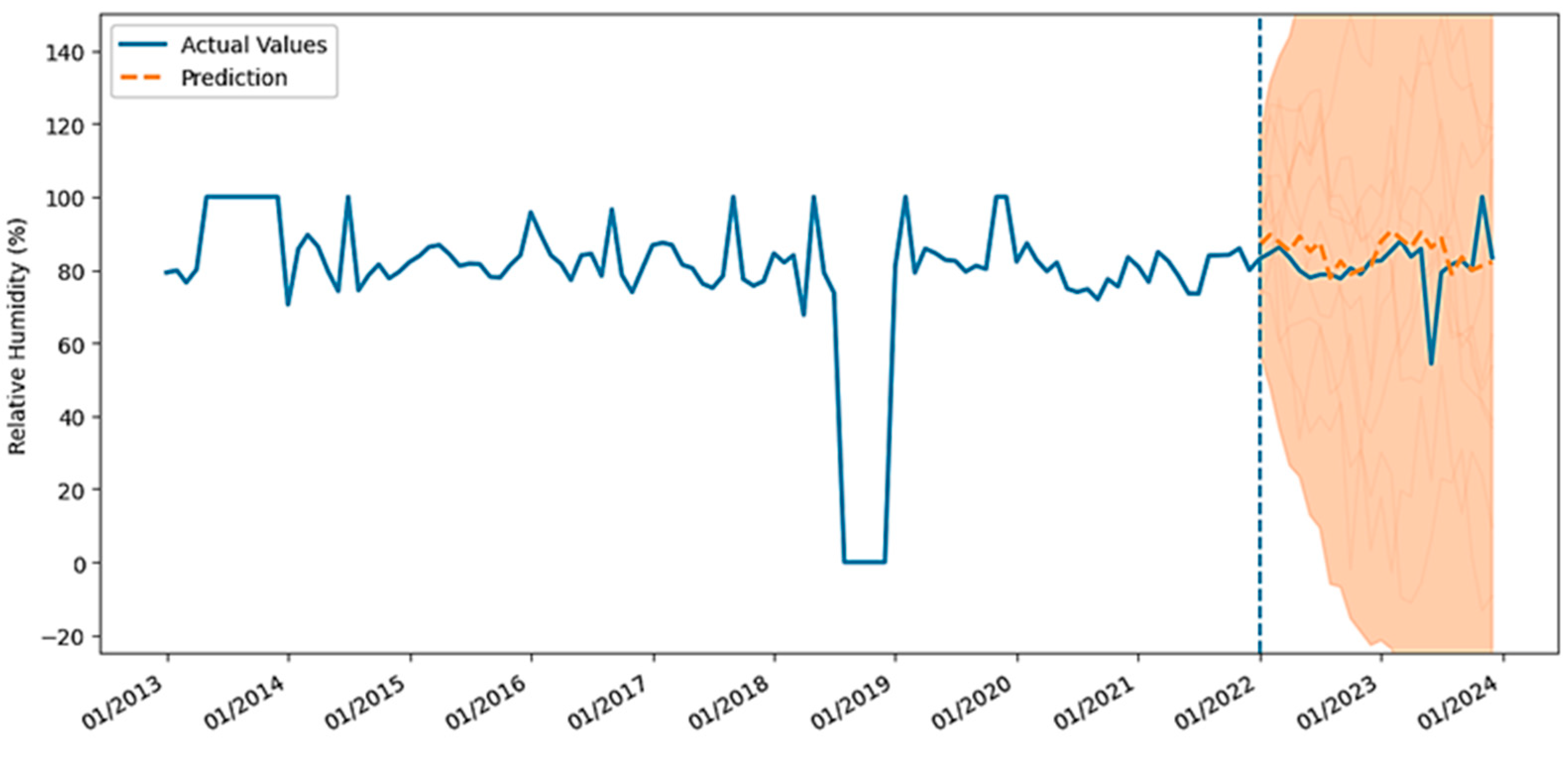
4.1.3. Relative Humidity (RH)

Monthly relative humidity data are obtained from the average of daily data from 2013 to 2023. Figure 9 illustrates the historical variability and predicted monthly mean RH at Cuchoquesera reservoir. The blue line represents the real variability, showing that there are months that reach 100%, with this phenomenon being more prolonged in 2013 between April and December; while in 2019, there are months with 0% between June and December, likely due to climatic factors or missing data. The prediction line shows an oscillation around 85%, while the shaded area indicates a confidence interval, with a remarkable amplitude in the prediction.

Figure 10 illustrates the seasonal variation, highlighting recurrent patterns observed during the study period. The months with the highest humidity are between January and April, showing pronounced peaks, while the months from September to December reflect the lowest RH levels. The orange band in the graph represents a 95% confidence interval.

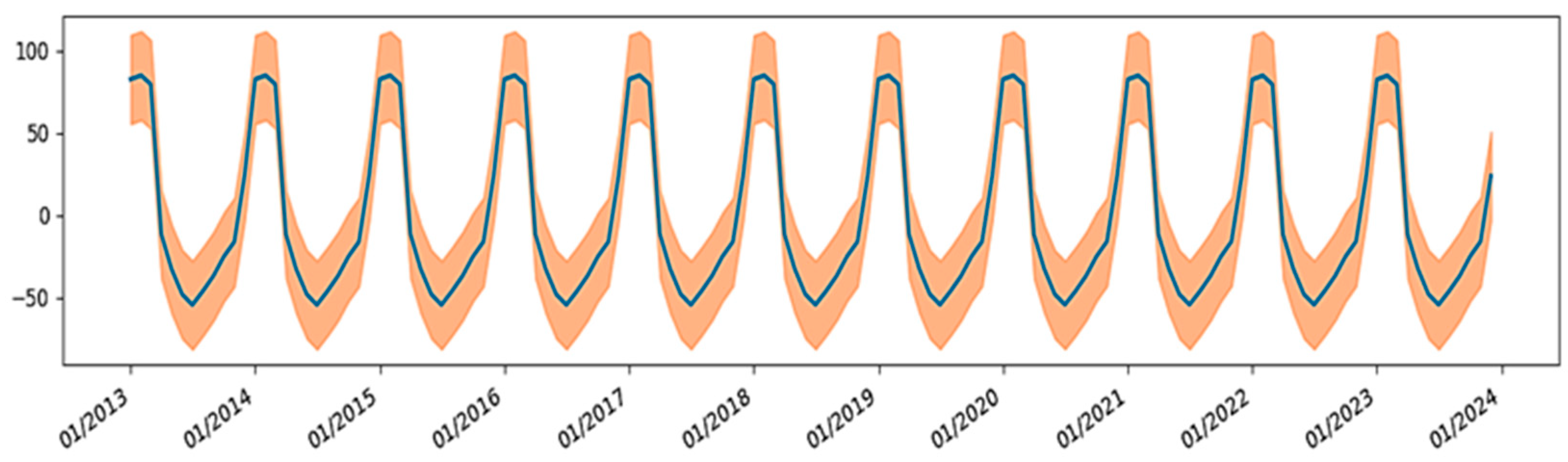
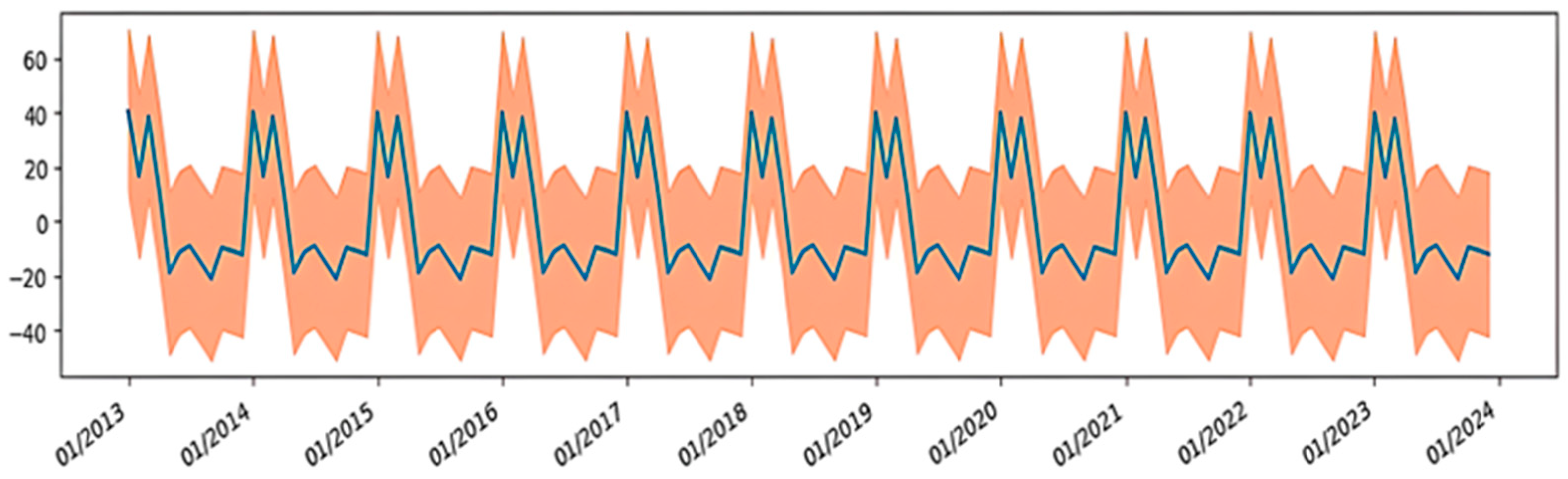
4.1.4. Ambient Temperature (Tamb)

Monthly ambient temperature data were obtained from the average of daily data from 2013 to 2023. Figure 11 illustrates the historical variability and predicted monthly mean Tamb at Cuchoquesera reservoir. The line representing the actual values oscillates at average temperatures of 10 °C for the majority of the period; however, higher temperatures are recorded between April and August 2019 and March 2020, reaching up to 18 °C, while minimum temperatures of 0 °C were especially pronounced between November and December 2019. The prediction line shows an oscillation between 10 and 12 °C. The shaded area represents a 95% confidence interval, with its width indicating variability in the prediction.

Figure 12 illustrates seasonal variation, highlighting recurring patterns observed during the study period. The months with the highest temperatures are between February and March, with less pronounced peaks occurring in November, and then rising and repeating the cycle. The orange band on the graph represents a confidence interval indicating the uncertainty for informed decision-making.

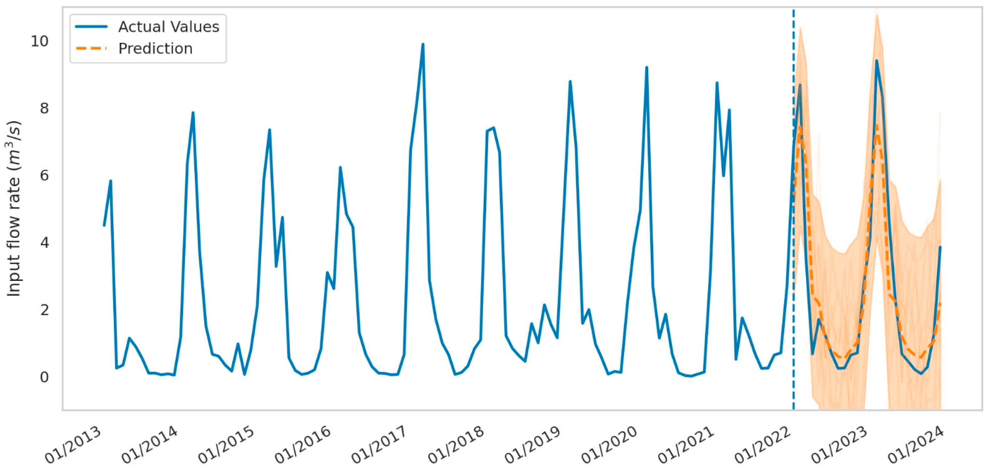
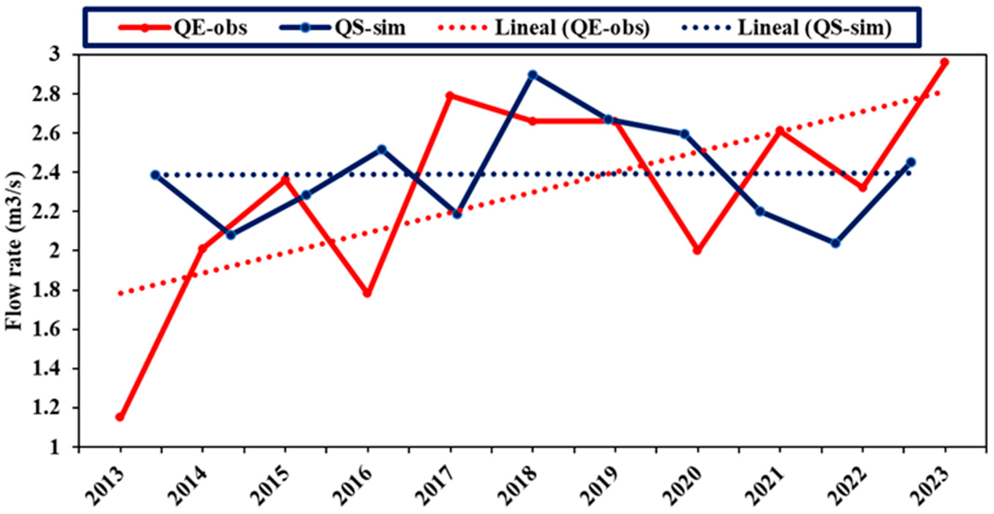
4.1.5. Observed Inflow (QE_obs)

Monthly inflow data are obtained from the average of the daily data from 2013 to 2023. Figure 13 illustrates the historical variability and predicted monthly mean QE_obs at Cuchoquesera reservoir. The blue line represents the actual values, showing that between January and April of each year, a higher QE_obs is recorded, reaching a maximum of 10 m³/s in 2017. Subsequently, the QE_obs decreases to its minimum value between June and November, again rising and repeating the cycle annually. The orange prediction line shows a behavior similar to the real values, where the bandwidth is narrower at the maximum peaks.

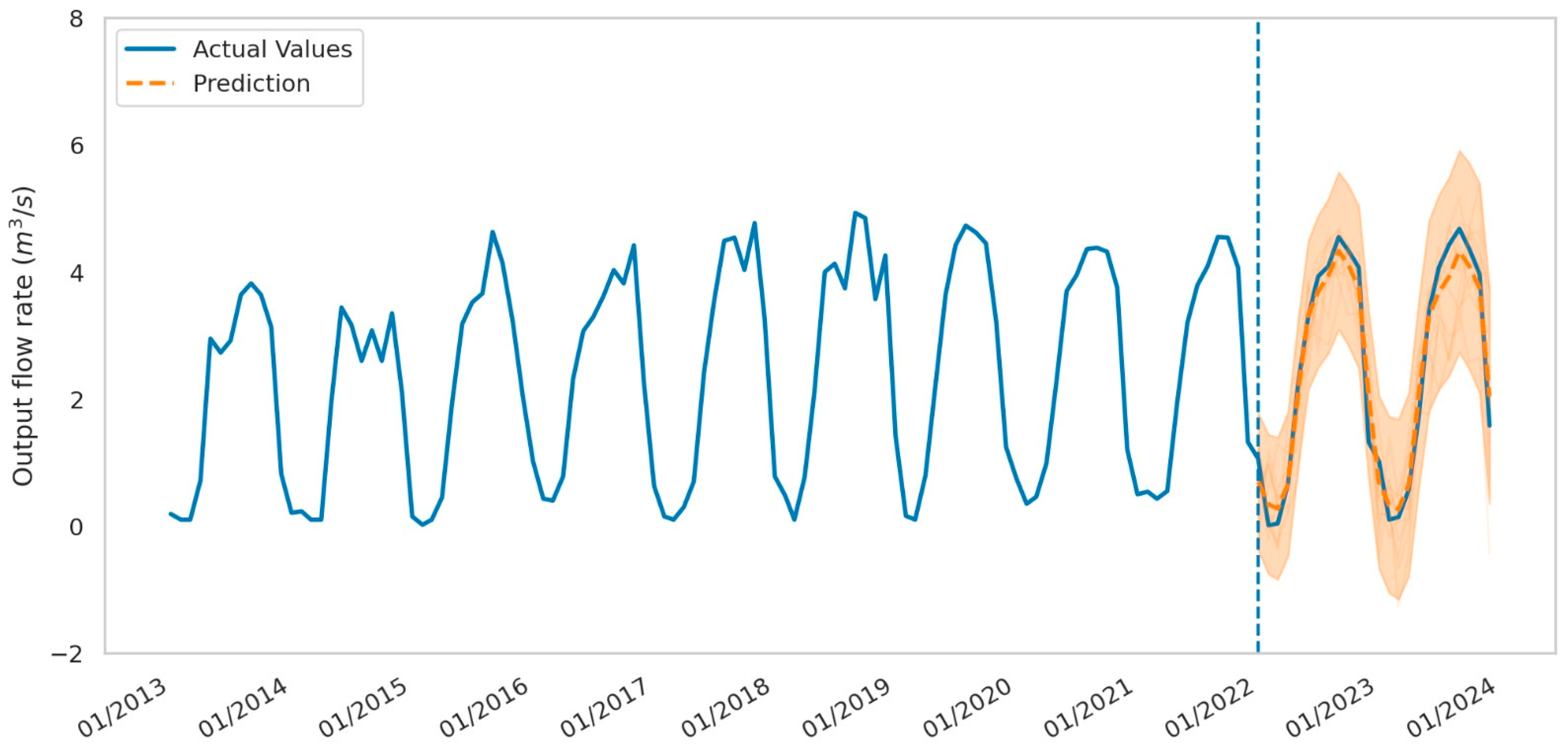
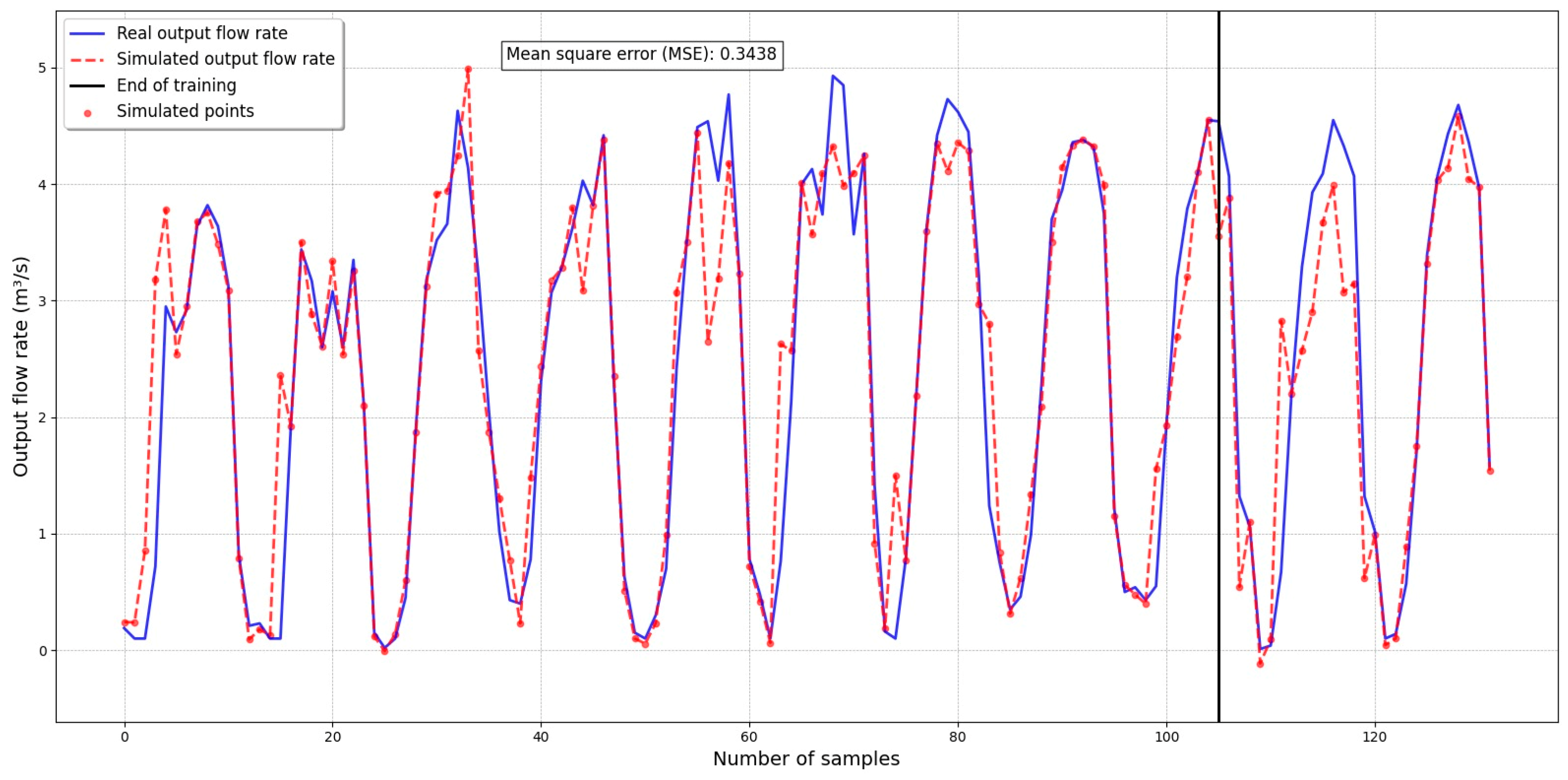
4.1.6. Observed Outflow (QS_obs)

Monthly QS_obs data were obtained from the average of daily data from January 2013 to December 2023. Figure 14 illustrates the historical variability and forecast of the monthly mean QS_obs in the Cuchoquesera reservoir. The actual values show an annual pattern, starting between January and March with a minimum value close to 0 m³/s, rising between June and August to reach a maximum of 4.2 m³/s, and falling again between September and December, repeating the cycle yearly.

To obtain the simulated output flow rate (QS_sim), the algorithm uses the Numpy packages for mathematical operations, Pandas for data reading and manipulation, Matplotlib for data visualization using graphs, and scikit-learn for the implementation of the multilayer Perceptron and the calculation of the mean square error. Subsequently, the input and output data are divided into 80% for training and 20% for testing, using a random state of 500 and implementing 1000 neurons in a single hidden layer. A sigmoid logistic activation function is used for continuous prediction, and finally, a maximum of 10,000 iterations is set for training to converge to an optimal solution, with a random state of 50.

Figure 15 shows the result of the water balance, where the data of the time series before the vertical line (black) correspond to the training, showing how the QS_sim follows the behavior of the QS_obs, which implies a similar behavior between both, recreating the moments of growth and decrease. The data in the continuous blue curve after the vertical black line represent the test data, used for model calibration and obtaining the red dashed curve corresponding to the QS_sim, with a mean squared error (MSE) of 0.3427, indicating a slight variation between the observed and simulated values over the study period.

Figure 16 shows a linear trend between QS_obs and QS_sim data through a scatter plot, which is represented by each pair of points (QS_obs, QS_sim), allowing for observation of the agreement between observed and simulated data. A black identity line with slope (m = 1) has been added, indicating the ideal relationship between the observed and simulated values. The proximity of the values to this line confirms that the model predicts values close to the observed or measured in situ values. However, some values show deviations, represented by the red trend line. The simulated values overestimate the QS_obs in the range 0 to 2.4 m³/s and underestimate them in the range 2.4 to 5.0 m³/s. The MLP model obtained an R² of 0.8739, indicating a strong relationship between the observed and simulated data, where 87% of the variability of the simulated data is explained by the QS_obs data, and the remaining 13% is due to complex variations that are not captured by the model.

To determine whether the model used is efficient, we determine the different validation indicators in

Table 3. Validation indicators of the simulated flow with respect to the observed flow.

Indicator	Result	Evaluation Range	Ideal Value
Nash–Sutcliffe Efficiency (NSE)	0.871	$\left[-\infty ;1\right]$	$1$
Nash–Sutcliffe-Ln Coefficient (NSE-Ln)	0.830	$\left[-\infty ;1\right]$	$1$
Pearson correlation coefficient	0.935	$\left[-1;1\right]$	$1$
Coefficient of determination (R2)	0.874	$\left[0;1\right]$	$1$
Root Mean Squared Error (RMSE)	0.244	$\left[0;+\infty \right]$	$0$
Bias-Score (Bs)	0.999	$\left[0;1\right]$	$1$
Relative Volume Error (RVB)	0.005	$\left[-\infty ;+\infty \right]$	$0$
Normalized Peak Value Error (NPE)	0.010	$\left[-\infty ;+\infty \right]$	$0$
Percentage of relative bias (PBIAS)	0.143	$\left[-\infty ;+\infty \right]$	$0$

.

The validation indicators are used to assess the performance of the model against the observed data and simulated values, based on interpretations aligned with criteria established by various authors, such as [48]. The Nash–Sutcliffe Efficiency (NSE = 0.871) suggests that the model has a good predictive capacity. The logarithmic Nash–Sutcliffe Efficiency (NSE-Ln = 0.830) indicates that the simulated discharge values (QS_sim) are close to the observed values (QS_obs), particularly under low-flow conditions. The Pearson correlation coefficient (r_xγ = 0.935) suggests a strong positive linear relationship between the QS_sim and QS_obs variables. The coefficient of determination R² = 0.874 indicates that 87% of the variability in the observed flow is explained by the model. The Root Mean Squared Error (RMSE = 0.244) indicates a low overall deviation between the values of QS_obs and QS_sim. The bias ratio (Bs = 0.999) suggests the model fits the observed values well, showing virtually no systematic bias. The Relative Volume Bias (RVB = 0.005) indicates that the total simulated volume is close to the observed one. The Normalized Peak Error (NPE = 0.010) indicates that the simulated peak discharge slightly overestimates the observed peak. The Percent Bias (PBIAS = 0.143) indicates that the model is moderately biased, likely due to uncertainties in measurements and data acquisition.

For a deeper analysis of the results, the annual linear trends of QE_obs and QS_sim between 2013 and 2023 were plotted, as shown in Figure 17, revealing a positive linear trend in both parameters. A greater slope is observed in the QE_obs with respect to the QS_sim, so that, between 2013 and 2019, QE_obs was lower than QS_sim, indicating that water inflow to the reservoir was less than the amount that left. On the other hand, between 2019 and 2023, QE_obs exceeded QS_sim, suggesting that during those years, inflow to the reservoir was greater than outflow. It is possible that, in the future, this behavior may persist due to various climatic factors, such as increased rainfall in the area where the Cuchoquesera reservoir is located.

For the water impoundment losses in the Cuchoquesera reservoir, the inflows and observed and simulated flows are considered. Thus, the differences between QS_obs and QE_obs (Figure 18) and QS_sim–QE_obs (Figure 19) are calculated.

Data values greater than 0 in both graphs indicate that more water is entering the reservoir than is leaving, suggesting that the Cuchoquesera reservoir is gaining water, influenced by various climatic factors, such as Pp. On the other hand, bars below 0 indicate that more water is leaving the reservoir than is entering, indicating that the reservoir is losing water due to infiltration and evapotranspiration, or other external factors. Water gains in the Cuchoquesera reservoir occur between January and April, while water losses are more prolonged from May to December.

5. Discussion

The objectives of this project have been achieved. The MLP model was proposed for water loss forecasting, based on historical hydrometeorological data recorded by the Sunilla station and compiled by OPEMAN, such as precipitation, evaporation, relative humidity, ambient temperature, and the inflow and outflow of the Cuchoquesera reservoir. With this data, a time series analysis was performed and the prediction was projected, as shown in Figure 4, which illustrates the relationship between the Pp and the inflow and outflow rates. With the exception of water losses, determined by the difference between the observed outflow (QS_obs) and inflow (QE_obs), as well as between the simulated outflow (QS_sim) and inflow (QE_obs), the other water components of the reservoir can be predicted using the same approach.

The estimated QS_sim of the water balance based on the MLP model can be replicated to simulate the behavior of the reservoirs in other dams, considering the use of HMPs characteristic of each dam and the objectives of the proposed research, in relation to the set of HMP data provided by the Cuchoquesera dam used in this model. In this way, it is possible to estimate the behavior of the reservoir, including storage, infiltration, and evaporation losses, as well as the annual trends of the inflow and outflow to the reservoir. Therefore, the information provided by the model offers sufficient scientific support for proposals to improve reservoir capacity performance through the integration of techniques for predicting damage and refurbishment of the dam, as well as for the effective management of water resources.

The validation indicators, which show NSE (0.8733), NSE-Ln (0.8303), Pearson (0.9348), R² (0.8739), RMSE (0.2435), Bias (0.9999), RVB (0.0048), NPE (0.0099), and PBIAS (0.1425), demonstrate that the model adequately simulates the output flow, although some variations could be improved:

(i)

Incomplete and missing data.

(ii)

Data errors resulting from the malfunctioning of sensors and instruments installed at the station.

The algorithm model developed in this work, with indicators (NSE = 0.87, RMSE = 0.24 m³/s, and R² = 0.87), is competitive compared to the deep learning model of [44], which obtained NSE = 0.87, RMSE = 0.20 m³/s, and R² = 0.91 for flow prediction. The difference is that the author uses more complex models with LSTM and Bayesian techniques, which require more time and are more expensive, but yield better sequence graphs in time series and can predict flows for future years.

The model also obtains a better NSE metric than those reported in univariate models, such as the model of [49], which obtained NSE between 0.75 and 0.85 using historical flow data. This could be due to the implementation of the HMP (Pp, Ev, RH, Tamb, QE_obs) in our MLP model, which captures nonlinear relationships. However, this model is still of great importance for catchments with limited instrumentation, where multivariate data collection is not feasible.

Another comparison is with [4], which achieved an RMSE of ±20.07% at Klang Gate Dam using an RBF neural network. The positive results could be attributed to the integration of meteorological variables, which outperform univariate approaches. For example, the authors of [50] integrated climatic data into their ANN study and were able to predict dissolved oxygen in the reservoir, with an R² = 0.98. These results suggest the potential of combining MLP with optimization algorithms to fine-tune water control policies.

Some deep learning models (CNN, LSTM, BiLSTM, GRU) [51] use Pp and flow data, for which the LSTM shows better efficiency, achieving an NSE between 0.85 and 0.90 and RMSE = 0.30 m³/s, compared to our model with an NSE of 0.87 and RMSE = 0.24 m³/s. It is evident that our model with historical data is limited compared to the LSTM model that captures peak flows. Future work could integrate LSTM to improve the resolution of the time series.

On the other hand, [3] uses seven models with input variable selection (IVS), including daily storage, reservoir, water discharge, and temporal factors. Among the models used, the recurrent neural network (RNN) with an RMSE testing of 14 m³/s stands out. Compared to our results, the RNN has better performance, taking into account that the data of our model are limited compared to the model of [3] that uses continuous data. This working approach suggests applying variables such as [3] to improve the accuracy of the model and thus better estimate water losses.

This water balance simulation model is capable of predicting or estimating water losses as well as the final storage of the reservoir. However, the accuracy of the model must be improved to minimize errors. By incorporating more historical data from the Cuchoquesera dam, the accuracy of the model can be improved. The best ANN performance for prediction depends not only on the amount of data, but also on the selection of the most significant number of neurons, transfer function types, and activation function used.

Therefore, it is possible to use other types of activation functions, such as recurrent neural networks and different combinations of transfer functions, to further develop the water balance model. From the simulated outflow (QS_sim) and inflow QE_obs, a trend line was obtained in both graphs, showing that both have a positive trend, with the slope of the QE_obs being greater. Finally, to estimate water losses, the difference between QS_obs and QS_sim with respect to QE_obs was calculated, which allowed the identification of the months in which water is lost or gained in the Cuchoquesera reservoir.

Unlike ref. [4], which used the initial and final monthly storage for network training from 2000 to 2007 to obtain a minimum model error, with this procedure the Machine Learning algorithm allowed the realization of the water balance and the projection or forecast of future events—mainly those related to the inflow and outflow parameters of the Cuchoquesera reservoir. Therefore, a deeper analysis can be carried out with data obtained from satellite stations, as well as taking into account the reservoir water storage in MCM. Finally, other computer programs such as RBF, TF, and other neural network models can be used to generate the water balance simulation model for the Cuchoquesera reservoir. A comparison between the ANN model and other models can be made to improve the model.

6. Conclusions

The proposed new Machine Learning algorithm enabled the development of a water balance model using data recorded at the Sunilla meteorological station and reservoir data from the Cuchoquesera dam. The model produced simulated output flow, which was validated with the measured or observed data at the reservoir. It was observed that the model tends to overestimate simulated output flow at low observed flow values and underestimate it at higher values.

In addition, the water balance model allowed the realization of a projection or forecast of the modelled input variables of precipitation, evaporation, inflow, relative humidity, and ambient temperature, verifying significant trends. The variation in the measured or observed inflow with respect to the simulated and observed outflow allowed for estimation of the reservoir losses due to evaporation and infiltration, showing that for values higher than zero, more water enters the reservoir than leaves it in the rainy stage, and for values lower than zero, more water leaves the reservoir than enters it. The losses due to evaporation and infiltration are more significant in the intermediate and dry stages.

References

- Raphaëlle, O.; Núñez, A.; Cathala, C.; Ríos, A.R.; Nalesso, M. Water in the Time of Drought II: Lessons from Droughts Around the World; Ntercambiar—América un Desarrollo Prohib: Washington, DC, USA, 2021; p. 56. [Google Scholar] [CrossRef]
- Where Is Earth’s Water?|U.S. Geological Survey. Available online: https://www.usgs.gov/special-topics/water-science-school/science/where-earths-water (accessed on 29 April 2025).
- Wannasin, C.; Brauer, C.C.; Uijlenhoet, R.; Torfs, P.J.J.F.; Weerts, A.H. Machine Learning for Real-Time Reservoir Operation Simulation: Comparing Input Variables and Algorithms for the Sirikit Reservoir, Thailand. J. Hydroinformatics 2024, 26, 3151–3171. [Google Scholar] [CrossRef]
- Dashti Latif, S.; Najah Ahmed, A.; Sherif, M.; Sefelnasr, A.; El-Shafie, A. Reservoir Water Balance Simulation Model Utilizing Machine Learning Algorithm. Alex. Eng. J. 2021, 60, 1365–1378. [Google Scholar] [CrossRef]
- Hurtado Asto, J.J. Análisis Hidrológico y Estimación del Balance Hídrico Para la Presa de Relaves Pataz—La Libertad—2019. Master’s Thesis, Universidad Ricardo Palma, Lima, Peru, 2019. [Google Scholar]
- Wang, K.; Shi, H.; Chen, J.; Li, T. An Improved Operation-Based Reservoir Scheme Integrated with Variable Infiltration Capacity Model for Multiyear and Multipurpose Reservoirs. J. Hydrol. 2019, 571, 365–375. [Google Scholar] [CrossRef]
- Zheng, Y.; Zhang, J.; Cheng, C.; Cao, H.; Yang, Y. Capacity Configuration of Hydropower-PV Complementary Station That Is Robust to the Inter-Annual Variability in Streamflow and PV Energy. Renew. Energy 2025, 248, 123163. [Google Scholar] [CrossRef]
- Fälth, H.E.; Hedenus, F.; Reichenberg, L.; Mattsson, N. Through Energy Droughts: Hydropower’s Ability to Sustain a High Output. Renew. Sustain. Energy Rev. 2025, 214, 115519. [Google Scholar] [CrossRef]
- Prado, I.G.; de Souza, M.A.; Coelho, F.F.; Pompeu, P.S. Dam Impact on Fish Assemblages Associated with Macrophytes in Natural and Regulated Floodplains of Pandeiros River Basin. Limnol. Rev. 2024, 24, 437–449. [Google Scholar] [CrossRef]
- Wisser, D.; Frolking, S.; Douglas, E.M.; Fekete, B.M.; Schumann, A.H.; Vörösmarty, C.J. The Significance of Local Water Resources Captured in Small Reservoirs for Crop Production—A Global-Scale Analysis. J. Hydrol. 2010, 384, 264–275. [Google Scholar] [CrossRef]
- Baalousha, H.M. Using Monte Carlo Simulation to Estimate Natural Groundwater Recharge in Qatar. Model. Earth Syst. Environ. 2016, 2, 87. [Google Scholar] [CrossRef]
- Chlost, I. Water Balance of Lake Gardno. Limnol. Rev. 2019, 19, 15–23. [Google Scholar] [CrossRef]
- Gurgiser, W.; Marzeion, B.; Nicholson, L.; Ortner, M.; Kaser, G. Modeling Energy and Mass Balance of Shallap Glacier, Peru. Cryosphere 2013, 7, 1787–1802. [Google Scholar] [CrossRef]
- Rabatel, A.; Francou, B.; Soruco, A.; Gomez, J.; Cáceres, B.; Ceballos, J.L.; Basantes, R.; Vuille, M.; Sicart, J.-E.; Huggel, C.; et al. Current State of Glaciers in the Tropical Andes: A Multi-Century Perspective on Glacier Evolution and Climate Change. Cryosphere 2013, 7, 81–102. [Google Scholar] [CrossRef]
- Sulca, J.; Vuille, M.; Dong, B. Interdecadal Variability of the Austral Summer Precipitation over the Central Andes. Front. Earth Sci. 2022, 10, 954954. [Google Scholar] [CrossRef]
- The Effect of El Niño on Weather in the Andes|GRID-Arendal. Available online: https://www.grida.no/resources/12828 (accessed on 26 April 2025).
- Krois, J.; Schulte, A.; Vigo, E.P.; Moreno, C.C. Temporal and spatial characteristics of rainfall patterns in the Northern Sierra of Peru—A case study for La Niña to El Niño transitions from 2005 to 2010. Espac. Desarro. 2013, 25, 23–48. [Google Scholar]
- Buytaert, W.; De Bièvre, B. Water for Cities: The Impact of Climate Change and Demographic Growth in the Tropical Andes. Water Resour. Res. 2012, 48, W08503. [Google Scholar] [CrossRef]
- Autoridad Administrativa del Agua Mantaro. Estudio de Prospección Batimétrica de la Represa Cuchoquesera; ANA-AAA X MANTARO; ANA—San Juan de Cuchoquesera-Ayacucho: Tokyo, Japan, 2016; p. 30. [Google Scholar]
- Soria-Lopez, A.; Sobrido-Pouso, C.; Mejuto, J.C.; Astray, G. Assessment of Different Machine Learning Methods for Reservoir Outflow Forecasting. Water 2023, 15, 3380. [Google Scholar] [CrossRef]
- Castro-Diaz, L.; García, M.A.; Villamayor-Tomas, S.; Lopez, M.C. Impacts of Hydropower Development on Locals’ Livelihoods in the Global South. World Dev. 2023, 169, 106285. [Google Scholar] [CrossRef]
- Ahmed, A.A.; Sayed, S.; Abdoulhalik, A.; Moutari, S.; Oyedele, L. Applications of Machine Learning to Water Resources Management: A Review of Present Status and Future Opportunities. J. Clean. Prod. 2024, 441, 140715. [Google Scholar] [CrossRef]
- Hassan-Esfahani, L.; Torres-Rua, A.; McKee, M. Assessment of Optimal Irrigation Water Allocation for Pressurized Irrigation System Using Water Balance Approach, Learning Machines, and Remotely Sensed Data. Agric. Water Manag. 2015, 153, 42–50. [Google Scholar] [CrossRef]
- Moncada, W.; Pereda, A.; Masías, M.; Lagos, M.; Portal-Quicaña, E.; Aldana, C.; Saavedra, Y.; Saavedra, E. Estimation of Soil Moisture of a High Andean Wetland Ecosystem (Bofedal) with Geo-Radar Data and In-Situ Measurements, Ayacucho—Peru. Int. Soil Water Conserv. Res. 2024, 13, 122–133. [Google Scholar] [CrossRef]
- Moncada, W.; Willems, B. Spatial and Temporal Analysis of Surface Temperature in the Apacheta Micro-Basin Using Landsat Thermal Data. Rev. Teledetección 2020, 57, 51–63. [Google Scholar] [CrossRef]
- Mathematical and Machine Learning Models for Groundwater Level Changes: A Systematic Review and Bibliographic Analysis. Available online: https://www.mdpi.com/1999-5903/14/9/259 (accessed on 28 April 2025).
- Osso Rodríguez, M.C.; Cabrales Arevalo, S.; Rosso Murillo, J.W. Diseño metodológico para la simulación del balance hídrico de una represa: Caso Tunja, Colombia. Rev. Científica 2017, 29, 230–248. [Google Scholar]
- Vargas Crispin, W.S.; Montes Raymundo, E.; Castrejón Valdez, M.; Hinojosa Benavides, R.A. Machine Learning como Herramienta para Determinar la Variación de los Recursos Hídricos. Sci. Res. J. CIDI 2021, 1, 56–69. [Google Scholar] [CrossRef]
- Fathian, F.; Mehdizadeh, S.; Kozekalani Sales, A.; Safari, M.J.S. Hybrid Models to Improve the Monthly River Flow Prediction: Integrating Artificial Intelligence and Non-Linear Time Series Models. J. Hydrol. 2019, 575, 1200–1213. [Google Scholar] [CrossRef]
- Marín Vilca, D.G.; Pineda Torres, I.A. Modelo predictivo Machine Learning Aplicado a Análisis de Datos Hidrometeorológicos Para un SAT en Represas. Mater’s Thesis, Universidad Tecnológica del Perú, Lima, Peru, 2019. [Google Scholar]
- Qian, X.; Qi, H.; Shang, S.; Wan, H.; Wang, R. Estimating Distributed Autumn Irrigation Water Use in a Large Irrigation District by Combining Machine Learning with Water Balance Models. Comput. Electron. Agric. 2024, 224, 109110. [Google Scholar] [CrossRef]
- Zhang, W.Y.; Xie, J.F.; Wan, G.C.; Tong, M.S. Single-Step and Multi-Step Time Series Prediction for Urban Temperature Based on LSTM Model of TensorFlow. In Proceedings of the 2021 Photonics & Electromagnetics Research Symposium (PIERS), Hangzhou, China, 21–25 November 2021; pp. 1531–1535. [Google Scholar]
- Kratzert, F.; Klotz, D.; Herrnegger, M.; Sampson, A.K.; Hochreiter, S.; Nearing, G.S. Toward Improved Predictions in Ungauged Basins: Exploiting the Power of Machine Learning. Water Resour. Res. 2019, 55, 11344–11354. [Google Scholar] [CrossRef]
- Sang, C.; Di Pierro, M. Improving Trading Technical Analysis with TensorFlow Long Short-Term Memory (LSTM) Neural Network. J. Financ. Data Sci. 2019, 5, 1–11. [Google Scholar] [CrossRef]
- Rozos, E.; Dimitriadis, P.; Bellos, V. Machine Learning in Assessing the Performance of Hydrological Models. Hydrology 2022, 9, 5. [Google Scholar] [CrossRef]
- Moriasi, D.N.; Arnold, J.G.; van Liew, M.W.; Bingner, R.L.; Harmel, R.D.; Veith, T.L. Model Evaluation Guidelines for Systematic Quantification of Accuracy in Watershed Simulations. Trans. ASABE 2007, 50, 885–900. [Google Scholar] [CrossRef]
- Gobierno Regional de Ayacucho. Proyecto Especial “Rio Cachi”; GORE-Ayacucho: Ayacucho, Perú, 2006; p. 47. [Google Scholar]
- Mitchell, T.M. Machine Learning (McGraw-Hill International Editions Computer Science Series), 1st ed.; McGraw-Hill Education: New York, NY, USA, 1997; ISBN 978-0-07-115467-3. [Google Scholar]
- Raschka, S.; Mirjalilli, V. Aprendizaje Automático con Python; Segunda Edición; MARCOMBO: Barcelona, Spain, 2019; ISBN 978-84-267-2720-6. [Google Scholar]
- Corona, J.C.; Diez, H.G.; Morell, C. Un estudio empírico del modelo de red neuronal MLP para problemas de predicción con salidas múltiples. Ser. CientíFica La Univ. Las Cienc. Inf. Áticas 2020, 13, 1–14. [Google Scholar]
- Myllis, G.; Tsimpiris, A.; Aggelopoulos, S.; Vrana, V.G. High-Performance Computing and Parallel Algorithms for Urban Water Demand Forecasting. Algorithms 2025, 18, 182. [Google Scholar] [CrossRef]
- Torres, J.F.; Martínez-Álvarez, F.; Troncoso, A. A Deep LSTM Network for the Spanish Electricity Consumption Forecasting. Neural Comput. Appl. 2022, 34, 10533–10545. [Google Scholar] [CrossRef]
- Qin, J.; Liang, J.; Chen, T.; Lei, X.; Kang, A. Simulating and Predicting of Hydrological TimeSeries Based on TensorFlow Deep Learning. Pol. J. Environ. Stud. 2018, 28, 795–802. [Google Scholar] [CrossRef] [PubMed]
- Lee, T.; Singh, V.P.; Cho, K.H. Tensorflow and Keras Programming for Deep Learning. In Deep Learning for Hydrometeorology and Environmental Science; Water Science and Technology Library; Springer International Publishing: Cham, Switzerland, 2021; Volume 99, pp. 151–162. ISBN 978-3-030-64776-6. [Google Scholar]
- Seo, J.Y.; Lee, S.-I. Predicting Changes in Spatiotemporal Groundwater Storage Through the Integration of Multi-Satellite Data and Deep Learning Models. IEEE Access 2021, 9, 157571–157583. [Google Scholar] [CrossRef]
- Zhang, J.; Zhu, Y.; Zhang, X.; Ye, M.; Yang, J. Developing a Long Short-Term Memory (LSTM) Based Model for Predicting Water Table Depth in Agricultural Areas. J. Hydrol. 2018, 561, 918–929. [Google Scholar] [CrossRef]
- Campos Aranda, D.F. Procesos del Ciclo Hidrológico; Universidad Autónoma de San Luis Potosí: San Luis Potosí, Mexico, 1998; ISBN 978-968-6194-44-9. [Google Scholar]
- García-Feal, O.; González-Cao, J.; Fernández-Nóvoa, D.; Astray Dopazo, G.; Gómez-Gesteira, M. Comparison of Machine Learning Techniques for Reservoir Outflow Forecasting. Nat. Hazards Earth Syst. Sci. 2022, 22, 3859–3874. [Google Scholar] [CrossRef]
- Zhang, Z.; Zhang, Q.; Singh, V.P. Univariate Streamflow Forecasting Using Commonly Used Data-Driven Models: Literature Review and Case Study. Hydrol. Sci. J. 2018, 63, 1091–1111. [Google Scholar] [CrossRef]
- Ziyad Sami, B.F.; Latif, S.D.; Ahmed, A.N.; Chow, M.F.; Murti, M.A.; Suhendi, A.; Ziyad Sami, B.H.; Wong, J.K.; Birima, A.H.; El-Shafie, A. Machine Learning Algorithm as a Sustainable Tool for Dissolved Oxygen Prediction: A Case Study of Feitsui Reservoir, Taiwan. Sci. Rep. 2022, 12, 3649. [Google Scholar] [CrossRef]
- Workneh, H.A.; Jha, M.K. Utilizing Deep Learning Models to Predict Streamflow. Water 2025, 17, 756. [Google Scholar] [CrossRef]