


Abstract
A generalized -dimensional Hirota-type nonlinear wave equation is investigated by combining Lie point symmetry analysis, invariant reductions, exact traveling-wave construction, and the direct multiplier method. A potential formulation is introduced under an explicit decay condition that makes the nonlocal term well defined. The admitted point symmetries are re-derived from the prolonged invariance criterion, and several symmetry reductions are obtained, including mixed translations, a transverse shear, scaling, and a general traveling-wave phase. The reduced traveling-wave equation admits an affine Riccati representation with hyperbolic, trigonometric, rational, and Bernoulli-type branches under explicit parameter restrictions. The corresponding 3D, 2D, and density visualizations are retained to illustrate the resulting wave profiles. Zeroth-order multipliers are then used to construct local conserved vectors in divergence form. The analysis provides a verified symmetry and conservation-law framework for the proposed higher-dimensional Hirota-type extension and supplies exact solutions that can be used as analytical benchmarks. The transverse-variable reductions and the zeroth-order multiplier family are derived specifically for the present -dimensional potential equation, while the Riccati functional forms are used as standard representations rather than claimed as new special functions.
Keywords:
generalized (3+1)-dimensional Hirota-type equation; Lie point symmetries; group-invariant solutions; traveling-wave solutions; conserved vectors; Riccati method MSC:
35G20; 35C05; 35C07
1. Introduction
The theory of nonlinear partial differential equations (NLPDEs) describes a wide range of physical phenomena including fluid mechanics, solid state physics, and plasma physics [1,2,3,4,5,6,7,8,9,10], with recent related developments reported in [11]. Exact solutions (closed-form solutions) of nonlinear partial differential equations are important for accurate description of qualitative characteristics of various processes and phenomena in many fields of natural sciences.
The famous Korteweg-de Vries equation [12]; recent analytical developments for KdV-type nonlinear-wave problems may also be found in [13]
governs solitary wave evolution. A solitary wave is a travelling wave solution that propagates without changing its shape. Waves that preserve their form after a collision are known as solitons [14]. Solitons come from a certain balance between nonlinearity and dispersion. The Korteweg-de Vries equation was originally derived to model shallow water waves with long wavelengths and small amplitudes. This equation is important for integrable systems because of its infinite conservation laws, multi-soliton solutions and many other physical features. The NLPDEs provide a graphical representation which helps to understand the mechanisms of some complex non linear phenomena e.g., spatial localisation of transfer processes. One of the most important areas of nonlinear study is the interaction of dispersive and nonlinear elements in nonlinear partial differential equations (NLPDEs) leading to solitons. This idea has many applications in different fields. Soliton events are important for the dynamics of nonlinear waves. These waves are important to mathematical and physical models because they keep their shape and speed over time.
The new generalised -dimensional Hirota bilinear equation
was studied in [15].
The lump–kink and lump–soliton interactions reported in [15], together with the higher-order breather and interaction structures in [16], motivate the study of higher-dimensional extensions of this Hirota-type model. The related -dimensional extension considered in [16] can be written as
By manipulating certain characteristic properties of the N-soliton solution, the resonance Y-type soliton and the interaction solution comprising the resonance Y-type soliton with the breathing solution and the lump solution were generated. Motivated by these studies, we consider the following generalized -dimensional Hirota-type extension:
We introduce the potential and impose . This condition is the natural decay (and gauge-fixing) requirement for the potential derivative at the left spatial boundary. Indeed, with a dummy integration variable , ; hence the imposed limit makes the nonlocal integral single-valued and equal to . For localized waves it is consistent with decay of the relevant potential derivative at spatial infinity.More precisely, the condition is imposed for every fixed . We assume on the domain of interest, is absolutely continuous in , and . Then the fundamental theorem of calculus gives . Whenever differentiation with respect to the remaining variables is interchanged with this improper integral, the corresponding derivatives are additionally assumed continuous and dominated by a locally uniform integrable majorant. These regularity and decay hypotheses make the localization step mathematically well defined. Hence , and the nonlocal equation is converted to the local potential equation
where , and are arbitrary non-zero constants.
Equation (5) is a local fifth-order nonlinear PDE obtained from the proposed higher-dimensional extension. The fifth-order mixed derivative provides the high-order dispersive contribution, the quadratic derivative products encode the nonlinearity, and the terms proportional to and represent additional linear dispersive couplings. Since the present work does not derive (4) from a specific fluid or plasma model, these interpretations are used at the structural level rather than as a claim of a unique physical realization.
The methods used in [15,16] focus mainly on explicit interaction solutions and do not provide the point-symmetry or multiplier structures sought here. We therefore apply Lie point symmetry analysis to the potential Equation (5), derive invariant reductions, construct traveling-wave solutions through an affine Riccati (Ma-type) ansatz, and determine local conservation laws by the direct multiplier method.
To place these steps more clearly in the literature, the symmetry calculation follows the standard Lie-group framework [17]; the lower-dimensional Hirota-type equations motivating the present extension are those in [15,16]. Higher-dimensional integrable or near-integrable structures and exact -dimensional nonlinear-wave solutions are represented by [3,4,6,18,19,20,21]. For conservation laws, the direct multiplier/Euler-operator approach is closely related to the systematic constructions in [22,23,24]. Because the nonlocal term is first converted to the local potential Equation (5), the multiplier analysis is performed entirely in local potential variables.
Recent applications further illustrate the use of analytical solution techniques, symmetry reductions, and Riccati-type mappings in nonlinear evolution models, including generalized Hirota–Satsuma–Ito dynamics, nonlinear metamaterial reductions, and soliton models in biomembranes and nerves [25,26,27].
The novelty claims are therefore deliberately limited and explicit. Relative to the lower-dimensional models [15,16], the generator and the -dependent generators – act on the additional transverse coordinate and have no literal counterpart in those -dimensional equations. The reductions in Cases 2–4 below exploit these transverse structures and are not reported in [15,16]; by contrast, the translation reductions in Cases 1 and 5 use standard symmetry mechanisms and are not claimed to be new as methods. The infinite zeroth-order multiplier family derived in Section 4 is a new result for the specific potential Equation (5), but we do not claim that infinite multiplier families are unique to the present dimensional extension. Finally, the hyperbolic, trigonometric, rational and Bernoulli functions generated from the Riccati equation are standard Riccati representatives; the new information here is their admissible embedding into the reduced ODE through the parameter map (60) and (61). The Möbius forms are explicitly treated as reparameterizations of the same Riccati branches rather than as independent new solution types.
The remainder of the paper is organized as follows. Section 2 presents the Lie point symmetries and group-invariant reductions. Section 3 develops the exact traveling-wave solutions and their graphical representations. Section 4 derives local conservation laws. Section 5 summarizes the main conclusions.
2. Lie Point Symmetries
We write the independent variables as and the dependent variable as . A generic one-parameter Lie point-symmetry generator is written in the standard compact form
where and are functions of . This notation separates each infinitesimal coefficient from its associated coordinate. The generator is a Lie point symmetry of (5) if
where is the fifth prolongation of (6). Expanding the above Equation (7) and splitting on the derivatives of leads to the following overdetermined system of linear partial differential equations:
Solving the determining system yields the following basis generators (with and arbitrary where indicated):
Group-Invariant Solutions of the Generalized -Dimensional Hirota-Type Equation
We now use representative one-dimensional subalgebras of the admitted symmetry algebra to construct similarity variables and reduce the number of independent variables. The first four cases illustrate reductions generated by mixed translations, the transverse shear, and scaling symmetries, whereas Case 5 develops the successive translation reduction that leads directly to the traveling-wave ODE used in Section 3.
All similarity reductions are understood locally on open sets where the selected generator has nonzero rank and the displayed invariants are functionally independent. In Case 1, is required and the one-phase subclass used for the fifth-order ODE assumes (equivalently ), so that . Case 2 is used away from the fixed set of , i.e., where . Case 3 requires because h contains . Case 4 is local on a region with (for a real-valued we take a fixed branch, e.g., ). In Case 5, the chosen invariants must have rank three, and the final traveling-wave reduction used in Section 3 requires and . Parameter choices violating these assumptions are excluded from the displayed formulas because they generate degenerate reductions that must be treated separately.
Case 1.
For the mixed translation generator
which is obtained from and the constant- member of , the characteristic equations give
Substitution into the potential Equation (5) yields
The indices in (36) follow directly from , , , and .
A useful one-phase invariant subclass is obtained by setting
where . In the original variables,
with
The reduced equation is
where
For , the real kink solution
satisfies (37) by direct substitution. This verified family replaces the previously stated expression containing the undefined parameter .
Case 2.
We then consider . The characteristic equations give the invariants
Substitution into (5) yields
The invariant follows from and removes the earlier ambiguity between the transverse coordinate and an auxiliary invariant.
Case 3.
We examine symmetry , and the characteristic equation produces invariants
Inserting these invariants into (5) yields
Equation (42) possesses four symmetries, specifically
It should be noted that and are arbitrary functions of f. We assume and consider a linear combination of and :
Solving the relevant characteristic equations associated with produces three invariants
Substituting into Equation (42) yields
Equation (46) possesses the following symmetries:
Linear combination simplifies (46) to a non-linear ordinary differential equation (ODE)
where Q is a function of .
Case 4.
For the scaling symmetry , the characteristic equations give
Indeed, , while , which is consistent with .
To write the reduced equation without introducing a long and error-prone expanded polynomial, define
Then, . Using also in the similarity variables, substitution of (49) into (5) gives the compact reduced PDE
All terms in (50) carry the common factor before it is divided out. This compact form is algebraically equivalent to the fully expanded reduction and makes the corrected invariant and the required factor explicit.
Case 5.
Consider the general translation generator , which is a constant-coefficient combination of the translation symmetries (with the constant member of supplying ). It reduces (5) to three independent variables and yields the invariants
Substitution of (51) into (5) gives a three-variable nonlinear PDE. Its fully expanded form is moved to Appendix A, Equation (A1), so that the reduction structure is visible in the main text. The reduced equation possesses the three translation symmetries
For the combination , convenient invariants are
The resulting two-variable PDE is listed in Appendix A, Equation (A2). It possesses the translations
Using their linear combination gives
The fully expanded fifth-order ODE is recorded in Appendix A, Equation (A3). Its nonlinear terms have the same coefficient, which is the structural feature used below.
For later use, Equation (A3) can be written compactly as
where is the coefficient of , is the coefficient of , and the two nonlinear coefficients in (A3) are identical. If
then direct factorization gives
This identity provides an independent check on the successive translation reductions.
The principal symmetry reductions are summarized in Table 1.
Table 1.
Summary of the symmetry reductions used in Section 2. The table distinguishes reductions that stop at a PDE from those that reach an ODE and an explicit solution.
3. Exact Solutions Using the Ma Method
This section reexamines the ansatz methodology [21,28] established by Ma for constructing exact solutions of nonlinear differential equations. Solitary-wave and periodic profiles expressed through hyperbolic and trigonometric functions are useful both for qualitative wave analysis and as benchmark solutions for numerical schemes.
To avoid confusing the traveling variable with the transverse coordinate , we use s throughout this section. Consider
where satisfies the Riccati equation
and are real constants.
Balancing with (or, equivalently, with ) in (56) gives
Thus
Since (56) contains only derivatives of F, is arbitrary. Substitution of (59) and (58) into (56), followed by coefficient comparison, yields the two compact conditions
and
These relations are the factored forms of the expanded parameter constraints generated by the successive reductions and eliminate unnecessary algebraic repetition.
Each Riccati branch can be verified at once by a symbolic residual. Define
Using and only the Riccati identity , direct symbolic differentiation and factorization give
Therefore (61) makes the residual identically zero, independently of which explicit Riccati representation is used. This verifies the hyperbolic, trigonometric, Möbius-equivalent and rational branches simultaneously. For the Bernoulli subclass , the same residual reduces to zero under .
The Ma construction is directly connected with the symmetry reductions in Section 2: Equation (56) is the canonical traveling-wave ODE obtained in Case 5 after the successive translation reductions. Case 1 has the same differential structure, with . In particular, setting in the hyperbolic Riccati branch gives by Equation (61), and hence
With and a shift of the phase origin, this is the same kink profile obtained in Case 1. Thus the Lie reductions determine the reduced traveling-wave equation, while Ma’s Riccati ansatz supplies explicit branches of that symmetry-reduced ODE.
Define the Riccati discriminant
The real branches are classified by the sign of .
For all formulas in this section we assume , and . The solutions are interpreted only on connected intervals on which every displayed denominator is nonzero; trigonometric branches are further restricted to intervals that do not cross poles of the tangent. These conditions specify the regularity domain of each benchmark solution.
First solution: hyperbolic branch. If ,
Second solution: trigonometric branch. If and ,
on intervals on which the tangent is finite.
A Möbius-equivalent trigonometric representation is
where P is an arbitrary constant and the denominator must be nonzero.
For , the corresponding Möbius-equivalent hyperbolic representation is
again away from zeros of the denominator.
Finally, when (equivalently ), the degenerate rational Riccati solution is
In every case the actual traveling-wave solution of (A3) is not alone but
with the parameter relation (61). Direct substitution into (56) gives zero identically.
For the Bernoulli equation,
which corresponds to , the affine representation remains valid whenever .
The first Bernoulli solution is
away from zeros of the denominator. A Möbius-equivalent representation is
again where the denominator is nonzero.
The resulting affine-Riccati branches and their admissibility conditions are summarized in Table 2.
Table 2.
Affine-Riccati traveling-wave branches and their admissibility conditions. In every row , with , , and .
The trigonometric formulas in (63) and (64) have been checked to contain tan, whereas the formulas (62) and (65) contain tanh; this is consistent with the discriminant classification and with the regularity statements in Table 2.
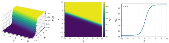
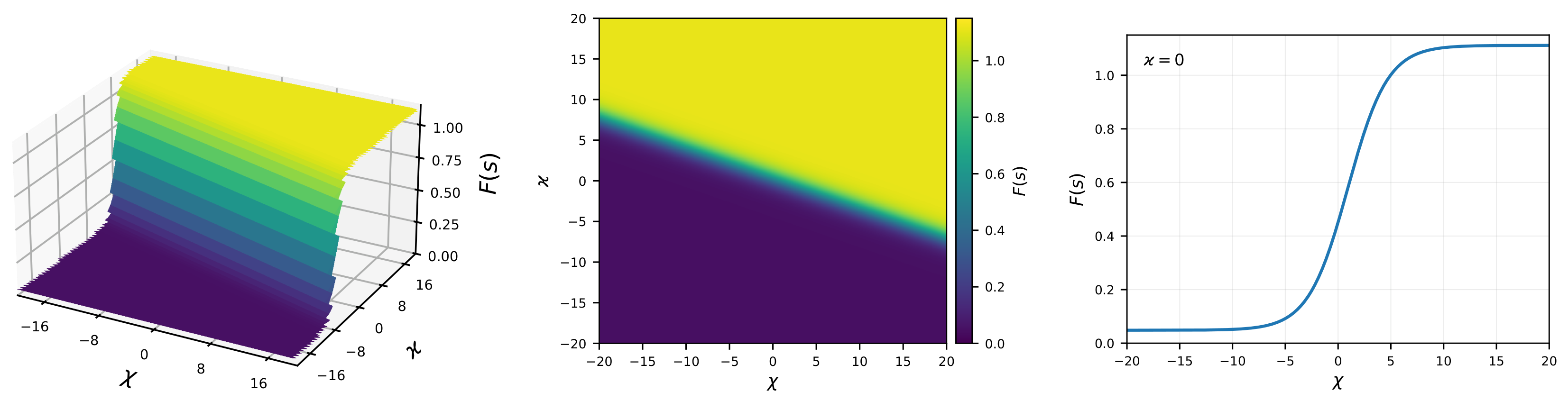
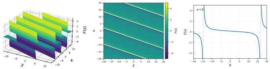
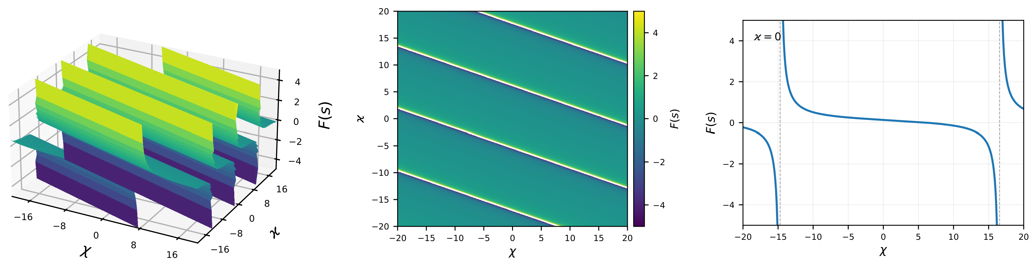
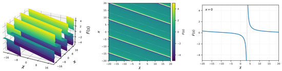
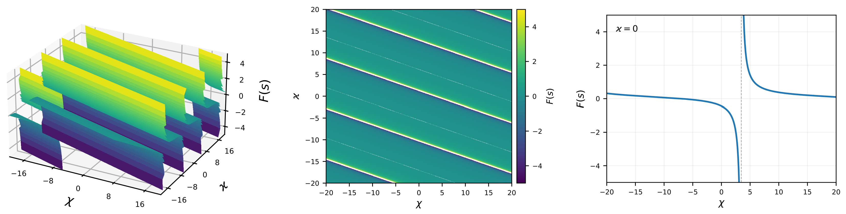
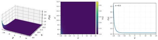
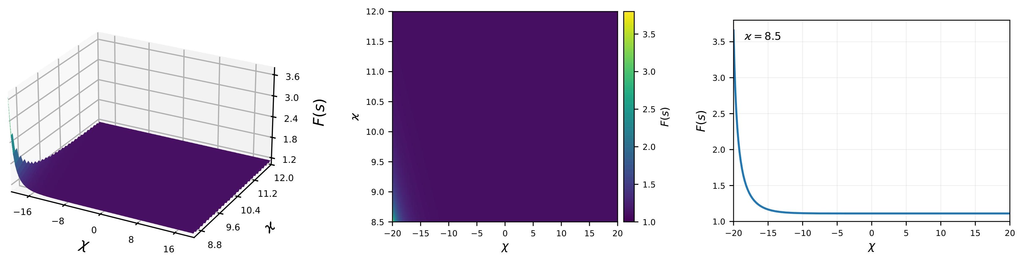
For Figure 1, Figure 2, Figure 3 and Figure 4, . With , Equation (61) holds for in Figure 1 and Figure 4 and in Figure 2 and Figure 3. All four figures are evaluated from Equations (62)–(65) with and . The 2D sections and displayed domains are stated in the captions.
Figure 2.
The 3D, density, and 2D profiles associated with the trigonometric branch (63) for the original parameter set . Direct evaluation of Equation (63) with : 3D/density, ; 2D, .Here ; the vertical dashed lines in the 2D panel mark the poles at and . Values with are omitted from the finite display window, not assigned finite values.
Figure 3.
The 3D, density, and 2D profiles associated with the Möbius-equivalent trigonometric branch (64) for the original parameter set . Direct evaluation of Equation (64) with : 3D/density, ; 2D, .Here ; the vertical dashed line marks the Möbius denominator zero at . The plotted formula excludes tangent poles and denominator zeros, and values with are omitted from the finite display window.
Figure 1, Figure 2, Figure 3 and Figure 4 visualize, respectively, the hyperbolic, trigonometric, Möbius-equivalent trigonometric, and Möbius-equivalent hyperbolic Riccati branches. In Figure 2 and Figure 3 the singular profiles are displayed only on their connected regularity intervals, with values outside the finite visualization window omitted from the graphics. They are local solutions of the potential Equation (5) on pole-free intervals; without an additional nonlocal formulation they are not asserted to satisfy the left-infinite-boundary condition used to derive it from the original integral equation.
4. Local Conservation Laws
Conservation laws provide structural information for differential equations and are useful in analytical reduction and structure-preserving numerical analysis [24,29]. For the potential Equation (5), a zeroth-order multiplier is characterized by the Euler-operator condition
where is the Euler operator, E denotes the left-hand side of (5), and is assumed to be of zeroth differential order. The analysis of (70) gives the following lemma.
Lemma 1.
Equation (5) admits an infinite family of zeroth-order multipliers of the form
where and are arbitrary smooth functions and H satisfies .
Proof.
Start with a general zeroth-order multiplier . Expanding the Euler identity and splitting with respect to independent jet variables gives, after elimination of redundant relations, the determining conditions needed here
The first group implies that the coefficient of depends only on and that the remaining part is at most quadratic in . Hence, we write
The relation gives . Setting therefore yields . The last determining equation reduces exactly to
while remains arbitrary. Consequently
A final substitution of this expression into the full Euler operator confirms when the displayed equation for H holds.□
For each admissible multiplier, the associated conserved vector satisfies the off-shell identity
The following conserved vectors are retained in expanded form:
Because the multiplier family contains arbitrary functions, (5) admits infinitely many local conservation laws. The family displayed here is of zeroth differential order. Higher-order multiplier searches may reproduce equivalent currents modulo trivial conserved vectors, but no claim of complete higher-order classification is required for the present result.
The conserved vectors provide exact divergence identities for the proposed PDE. In particular, choosing selects one member of the multiplier family, but it is not identified here as physical energy because no Hamiltonian or Noether interpretation has been established for the proposed higher-dimensional model. Under appropriate decay or periodic boundary conditions, nontrivial conserved integrals can be obtained from the corresponding time component after trivial divergence terms are removed.
5. Conclusions
A generalized -dimensional Hirota-type equation has been investigated through a local potential formulation, Lie point symmetry analysis, invariant reductions, exact traveling-wave solutions, and the direct multiplier method. The potential transformation was formulated together with the decay condition required for the consistent evaluation of the nonlocal integral. The admitted symmetry generators were carefully verified against the corresponding determining equations, including the time-dependent spatial-shift generator, while the mixed-translation, transverse-shear, scaling, and traveling-wave reductions were expressed in forms consistent with the potential equation.
The traveling-wave reduction leads to a nonlinear fifth-order ODE that admits an affine Riccati representation. Within this affine Riccati class, the method produces several explicit hyperbolic, trigonometric, rational, and Bernoulli-type solution families subject to the parameter and regularity restrictions summarized in Table 2. These families are not asserted to classify all traveling-wave solutions of the fifth-order ODE. Their validity follows from the factored symbolic residual given in Section 3, and the retained figures illustrate only branches that can be identified unambiguously with a specific analytical formula.
In addition, an infinite family of zeroth-order multipliers and corresponding local conserved vectors has been derived in divergence form. This is a classification within the stated zeroth-order multiplier ansatz, not a complete classification of all conservation laws; higher-order or non-equivalent multiplier families are not excluded. The conservation laws are presented without assigning an unsupported physical interpretation to a particular multiplier. The verified exact solutions can serve as analytical benchmarks for future numerical studies on the connected parameter intervals where their denominators remain nonzero and their stated regularity conditions hold.
Author Contributions
Y.G. and A.H.A.: writing—original draft preparation, visualization, investigation, and methodology; A.R.A., B.M. and S.O.M.: formal analysis, data curation, and software; A.B.: conceptualization, project administration, and funding acquisition. All authors have read and agreed to the published version of the manuscript.
Funding
This research received no external funding.
Data Availability Statement
All data supporting the findings of this study are included in the article.
Acknowledgments
The work of the last author (A.B.) was supported by Grambling State University through the Endowed Chair of Mathematics. The author gratefully acknowledges this support.
Conflicts of Interest
The authors declare no conflicts of interest.
Appendix A. Expanded Algebra for the Successive Translation Reduction
For auditability, the long expanded equations removed from the main text are collected here. They correspond exactly to the three-variable PDE, the two-variable PDE, and the final expanded fifth-order ODE generated in Case 5. The compact structural form used in the main text is Equation (56).
References
- Ma, W.-X. A combined derivative nonlinear Schrödinger soliton hierarchy. Rep. Math. Phys. 2024, 93, 313–325. [Google Scholar] [CrossRef] [Scilit]
- Ma, W.-X. N-soliton solution and the Hirota condition of a (2 + 1)-dimensional combined equation. Math. Comput. Simul. 2021, 190, 270–279. [Google Scholar] [CrossRef] [Scilit]
- Wazwaz, A.M. Multi-soliton solutions for integrable (3 + 1)-dimensional modified seventh-order Ito and seventh-order Ito equations. Nonlinear Dyn. 2022, 110, 3713–3720. [Google Scholar] [CrossRef] [Scilit]
- Wazwaz, A.M. New (3 + 1)-dimensional integrable fourth-order nonlinear equation: Lumps and multiple soliton solutions. Int. J. Numer. Methods Heat Fluid Flow 2022, 32, 1664–1673. [Google Scholar] [CrossRef] [Scilit]
- Wang, Y.; Lü, X. Bäcklund transformation and interaction solutions of a generalized Kadomtsev–Petviashvili equation with variable coefficients. Chin. J. Phys. 2024, 89, 37–45. [Google Scholar] [CrossRef] [Scilit]
- He, X.-J.; Lü, X. M-lump solution, soliton solution and rational solution to a (3 + 1)-dimensional nonlinear model. Math. Comput. Simul. 2022, 197, 327–340. [Google Scholar] [CrossRef] [Scilit]
- Rasoulizadeh, M.N.; Avazzadeh, Z.; Nikan, O. Solitary wave propagation of the generalized Kuramoto–Sivashinsky equation in fragmented porous media. Int. J. Appl. Comput. Math. 2022, 8, 252. [Google Scholar] [CrossRef] [Scilit]
- Nikan, O.; Avazzadeh, Z. An efficient localized meshless technique for approximating nonlinear sinh-Gordon equation arising in surface theory. Eng. Anal. Bound. Elem. 2021, 130, 268–285. [Google Scholar] [CrossRef] [Scilit]
- Nikan, O.; Golbabai, A.; Nikazad, T. Solitary wave solution of the nonlinear KdV–Benjamin–Bona–Mahony–Burgers model via two meshless methods. Eur. Phys. J. Plus 2019, 134, 367. [Google Scholar] [CrossRef] [Scilit]
- Li, M.; Nikan, O.; Qiu, W.; Xu, D. An efficient localized meshless collocation method for the two-dimensional Burgers-type equation arising in fluid turbulent flows. Eng. Anal. Bound. Elem. 2022, 144, 44–54. [Google Scholar] [CrossRef] [Scilit]
- Anco, S.C.; Márquez, A.P.; Garrido, T.M.; Gandarias, M.L. Symmetry analysis and hidden variational structure of Westervelt’s equation in nonlinear acoustics. Commun. Nonlinear Sci. Numer. Simul. 2023, 124, 107315. [Google Scholar] [CrossRef] [Scilit]
- Korteweg, D.J.; de Vries, G. On the change of form of long waves advancing in a rectangular canal and on a new type of long stationary waves. Lond. Edinb. Dublin Philos. Mag. J. Sci. 1895, 39, 422–443. [Google Scholar] [CrossRef] [Scilit]
- Márquez, A.P.; Garrido, T.M.; Khalique, C.M.; Gandarias, M.L. Symmetries, conservation laws, and line soliton solutions of a two-dimensional generalized KdV equation with p-power. Discret. Contin. Dyn. Syst.-Ser. S 2025, 18, 1024–1035. [Google Scholar] [CrossRef] [Scilit]
- Zabusky, N.J.; Kruskal, M.D. Interaction of “solitons” in a collisionless plasma and the recurrence of initial states. Phys. Rev. Lett. 1965, 15, 240–243. [Google Scholar] [CrossRef] [Scilit]
- Hua, Y.-F.; Guo, B.-L.; Ma, W.-X.; Lü, X. Interaction behavior associated with a generalized (2 + 1)-dimensional Hirota bilinear equation for nonlinear waves. Appl. Math. Model. 2019, 74, 184–198. [Google Scholar] [CrossRef] [Scilit]
- Zhao, Z.; He, L. M-lump, high-order breather solutions and interaction dynamics of a generalized (2 + 1)-dimensional nonlinear wave equation. Nonlinear Dyn. 2020, 100, 2753–2765. [Google Scholar] [CrossRef] [Scilit]
- Olver, P.J. Applications of Lie Groups to Differential Equations, 2nd ed.; Springer: New York, NY, USA, 1993. [Google Scholar]
- Mikhailov, A.V.; Shabat, A.B.; Yamilov, R.I. On an extension of the module of invertible transformations. Sov. Math. Dokl. 1988, 36, 60–63. [Google Scholar]
- Mikhailov, A.V.; Shabat, A.B.; Yamilov, R.I. Extension of the module of invertible transformations and classification of integrable systems. Commun. Math. Phys. 1988, 115, 1–19. [Google Scholar] [CrossRef] [Scilit]
- Kodama, Y.; Mikhailov, A.V. Obstacles to asymptotic integrability. In Algebraic Aspects of Integrable Systems; Fokas, A.S., Gelfand, I.M., Eds.; Birkhäuser: Boston, MA, USA, 1997; pp. 173–204. [Google Scholar]
- Ma, W.-X.; Lee, J.-H. A transformed rational function method and exact solutions to the (3 + 1)-dimensional Jimbo–Miwa equation. Chaos Solitons Fractals 2009, 42, 1356–1363. [Google Scholar] [CrossRef] [Scilit]
- Anco, S.C.; Bluman, G. Direct construction method for conservation laws of partial differential equations. Part I: Examples of conservation law classifications. Eur. J. Appl. Math. 2002, 13, 545–566. [Google Scholar] [CrossRef] [Scilit]
- Anco, S.C.; Bluman, G. Direct construction method for conservation laws of partial differential equations. Part II: General treatment. Eur. J. Appl. Math. 2002, 13, 567–585. [Google Scholar] [CrossRef] [Scilit]
- Ma, W.-X. Conservation laws by symmetries and adjoint symmetries. Discret. Contin. Dyn. Syst.-Ser. S 2018, 11, 725–739. [Google Scholar] [CrossRef] [Scilit]
- Iqbal, M.; Riaz, M.B.; Aziz ur Rehman, M.; Kazmi, S.S. Nonlinear dynamics of the generalized Hirota–Satsuma–Ito equation: Analytical solutions and graphical insights. Math. Comput. Simul. 2026, 239, 729–744. [Google Scholar] [CrossRef] [Scilit]
- Afridi, M.I. Stochastic dynamics of symmetry reductions to the parabolic nonlinear model in metamaterials. Results Eng. 2025, 26, 105630. [Google Scholar] [CrossRef] [Scilit]
- Rani, A.; Shakeel, M.; Sohail, M.U.; Mahariq, I. The generalizing Riccati equation mapping method’s application for detecting soliton solutions in biomembranes and nerves. Partial. Differ. Equ. Appl. Math. 2025, 15, 101300. [Google Scholar] [CrossRef] [Scilit]
- Ma, W.-X.; Fuchssteiner, B. Explicit and exact solutions to a Kolmogorov–Petrovskii–Piskunov equation. Int. J. Non-Linear Mech. 1996, 31, 329–338. [Google Scholar] [CrossRef] [Scilit]
- LeVeque, R.J. Numerical Methods for Conservation Laws, 2nd ed.; Birkhäuser: Basel, Switzerland, 1992. [Google Scholar]

Disclaimer/Publisher’s Note: The statements, opinions and data contained in all publications are solely those of the individual author(s) and contributor(s) and not of MDPI and/or the editor(s). MDPI and/or the editor(s) disclaim responsibility for any injury to people or property resulting from any ideas, methods, instructions or products referred to in the content. |
© 2026 by the authors. Licensee MDPI, Basel, Switzerland. This article is an open access article distributed under the terms and conditions of the Creative Commons Attribution (CC BY) license.