Artificial Neural Networks and Simulation of Nonlinear Soliton Solutions of the Modified Benjamin–Bona–Mahony Equation in Nonlinear Optics

Abstract

In order to investigate the soliton solutions of the third-order nonlinear modified Benjamin–Bona–Mahony equation, this research presents a hybrid analytical and machine-learning methodology. A novel combination of symbolic computation and data-driven modeling is introduced to strengthen the theoretical analysis and improve the simulation capabilities. Next, we propose a Riccati sub-equation neural network (RSENN) framework in which the traveling-wave transformation and Riccati sub-equation structure are incorporated into the neural network model. The proposed RSENN framework accurately approximates the soliton solutions and predicts their spatiotemporal evolution governed by the modified Benjamin–Bona–Mahony equation. The data-driven discovery of the model equation is also performed by estimating the unknown parameters under different noise intensities. The RSENN model is trained using the Levenberg–Marquardt algorithm, and its accuracy and predictive capability are evaluated by comparing its numerical outputs with the exact analytical solutions. The results demonstrate the robustness of the proposed RSENN approach under different levels of noise contamination.

1. Introduction

This section presents the background and overview of prior studies, emphasizes the key contributions of the work, identifies existing gaps in the literature, and describes the overall structure of the paper.

1.1. Background of the Study

The nonlinear partial differential equation (NLPDE) is initially transformed into a nonlinear ordinary differential equation using an appropriate transformation for further analysis. It regulates the changes in fluid and gas properties such as pressure, heat, and velocity. Many challenges remain unresolved because of the complex, high-order structure of NLPDEs, despite significant efforts to find exact and approximate solutions [1,2,3]. Finding analytical solutions to these equations provides important information for upcoming theoretical advancements in addition to illuminating the fundamental mechanics of nonlinear occurrences. Therefore, understanding complex systems with non-proportional and dynamic connections requires a firm grasp of nonlinear science [4,5,6,7]. Neural networks are highly expressible in approximation of functions [8], and using them for solving differential and integral equations has become a vital and popular study topic [9]. The application of physics-informed neural networks to solve PDEs has drawn a lot of attention.

Artificial neural networks can also be used to deal with NLPDEs and discover the inverse case with parameters that are unknown. The development of computational mathematical and engineering knowledge has been aided by the merging of these subjects with already established mathematical methods [10,11,12]. These solutions are accurate, dependable, and constrained, which greatly aids in understanding the role of nonlinear dynamics in complex physical systems. The Levenberg–Marquardt-Artificial Neural Network (LM-ANN) is a fast and efficient training algorithm used for solving nonlinear problems in neural networks. It combines the advantages of gradient descent and the Gauss–Newton method to achieve quicker convergence. LM-ANN is widely used in function approximation, prediction, and modeling due to its high accuracy and speed. Unlike existing hybrid analytical–neural approaches, the proposed RSENN framework does not merely use neural networks as approximators. Instead, it incorporates the known analytical solution structure into the learning process, allowing the network to learn only the residual correction. This reduces the learning burden, improves convergence, and enhances the accuracy of nonlinear wave prediction.

Solitons are not only special occurrences in mathematical physics but they also commonly represent the fundamental behaviors of objects in several paradigms [13,14]. Nonlinear dynamics and wave transmission are crucial areas of study in many different fields because of waves’ ability to retain their structure and energy after interacting with other waves [15]. Finding precise answers for a variety of scientific procedures might reveal their essential traits [16]. These approaches provide a platform for additional study, emphasizing their significance [17,18]. The actual structure’s fluctuations must be expressed as an ODE or PDE in order to obtain an exact solution. PDEs are frequently employed as mathematical models for intricate economic and biological phenomena. Researchers have developed a wide range of computational and analytical techniques to successfully handle these problems. As a result, several approaches have gained popularity over the last few decades because of their capacity to produce precise answers to NLPDEs. These methods incorporate the generalized Riccati equation mapping method [19], the modified F-expansion approach [20], the extended algebraic method [21], the inverse scattering transform [5], and others [22,23].

1.2. Comprehensive Analysis of the Mathematical Framework

In order to describe the propagation of persistent waves in nonlinear dispersive systems, the modified Benjamin–Bona–Mahony (mBBM) equation is frequently used [24]. It can be used to analyze internal waves in structured fluid media, ion-acoustic waves seen in plasma, and shallow water waves [25,26]. First, we provide a detailed description of all parameters and their abbreviations are summarized in

Table 1. Description of the parameters used in the model.

Parameter	Interpretation
$\mathcal{K},\mathcal{M}$	Velocity
${\kappa }_0$	Density
$\mathcal{Q}$	Pressure
${\mathcal{G}}_0$	Gravitational acceleration
${\mathcal{H}}^{★}$	Water depth
${\eta }_a$	Tiny parameter
${\mathcal{N}}^{★}$	Free surface elevation
$\mathcal{T}$	Time variable
$\mathcal{P}$	Dependent variable
$\alpha$	Space variable

. The Euler equations are successfully converted into the mBBM equation by using various presumptions and estimates:

$$\begin{array}{cc}\hfill & {\mathcal{K}}_{\mathcal{T}}+\mathcal{K}{\mathcal{K}}_{\alpha }+\mathcal{M}{\mathcal{K}}_{\gamma }=-{\displaystyle \frac{1}{{\kappa }_0}}{\mathcal{Q}}_{\alpha },\hfill \\ \hfill & {\mathcal{M}}_{\mathcal{T}}+\mathcal{K}{\mathcal{M}}_{\alpha }+\mathcal{M}{\mathcal{M}}_{\gamma }=-{\displaystyle \frac{1}{{\kappa }_0}}{\mathcal{Q}}_{\gamma }+{\mathcal{G}}_0.\hfill \end{array}$$

(1)

A horizontal, incompressible fluid, with an impermeable bottom is covered by an inflexible, oscillating fluid in a weakly nonlinear situation.Next, the continuity equation is provided by [27]

$${\mathcal{K}}_{\alpha }+{\mathcal{M}}_{\gamma }=0.$$

(2)

The subsequent non-dimensional variables were established by us:

$$\left\{\begin{array}{c}\begin{array}{c}{\alpha }^{\prime }={\displaystyle \frac{\alpha }{{\mathcal{H}}^{★}}},{\gamma }^{\prime }={\displaystyle \frac{\gamma }{{\mathcal{H}}^{★}}},{\mathcal{K}}^{\prime }={\displaystyle \frac{\mathcal{K}}{\sqrt{{\mathcal{G}}_0{\mathcal{H}}^{★}}}},{\mathcal{M}}^{\prime }={\displaystyle \frac{\mathcal{M}}{\sqrt{{\mathcal{G}}_0{\mathcal{H}}^{★}}{\eta }_a}},{\mathcal{Q}}^{\prime }={\displaystyle \frac{\mathcal{Q}}{{\kappa }_0\mathcal{G}{\mathcal{H}}^{★}}},\hfill \\ {\mathcal{T}}^{\prime }={\displaystyle \frac{\mathcal{T}}{\sqrt{{\mathcal{H}}^{★}{\mathcal{G}}^{-1}}}},{{\mathcal{N}}^{★}}^{\prime }={\displaystyle \frac{N}{{\mathcal{H}}^{★}}},\hfill \\ {{\mathcal{K}}^{\prime }}_{{\mathcal{T}}^{\prime }}+{\eta }_a\left({\mathcal{S}}^{\prime }{{\mathcal{K}}^{\prime }}_{{\alpha }^{\prime }}+{\mathcal{M}}^{\prime }{{\mathcal{K}}^{\prime }}_{{\gamma }^{\prime }}\right)={-N^{\prime }}_{{\alpha }^{\prime }},\hfill \\ {\eta }_a\left({{\mathcal{M}}^{\prime }}_{{\mathcal{T}}^{\prime }}+{\mathcal{K}}^{\prime }{{\mathcal{M}}^{\prime }}_{{\alpha }^{\prime }}+{\mathcal{M}}^{\prime }{{\mathcal{M}}^{\prime }}_{{\gamma }^{\prime }}\right)={-\partial N}_{{\gamma }^{\prime }},\hfill \\ {{\mathcal{K}}^{\prime }}_{{\alpha }^{\prime }}+{{\mathcal{M}}^{\prime }}_{{\gamma }^{\prime }}=0.\hfill \end{array}\hfill \end{array}\right.$$

(3)

Several modifications are then applied [28]:

$$\left\{\begin{array}{c}\begin{array}{c}{\mathcal{K}}^{\prime }={\mathrm{\Phi }}_{\alpha }^{\prime },S^{\prime }={\mathrm{\Phi }}_{\gamma }^{\prime },\hfill \\ N^{\prime }={\mathrm{\Phi }}_{\alpha {\alpha }^{\prime }}^{\prime }+{\mathrm{\Phi }}_{\gamma {\gamma }^{\prime }}^{\prime }.\hfill \end{array}\hfill \end{array}\right.$$

(4)

Putting Equation (4) into Equation (3) yields the mBBM equation:

$${\mathrm{\Phi }}_{{\alpha }^{\prime }{\alpha }^{\prime }{\mathcal{T}}^{\prime }}+{\mathrm{\Phi }}_{{\mathcal{T}}^{\prime }}+{\eta }_a{Q}_0{\mathrm{\Phi }}^2{\mathrm{\Phi }}_{{\alpha }^{\prime }}+{\mathrm{\Phi }}_{{\alpha }^{\prime }}=0·$$

(5)

The mBBM equation can be written in the following form [28]:

$${\mathcal{P}}_{\alpha \alpha \mathcal{T}}+{\mathcal{P}}_{\mathcal{T}}+Q_0{\mathcal{P}}^2{\mathcal{P}}_{\alpha }+{\mathcal{P}}_{\alpha }=0.$$

(6)

Here, $\mathcal{P}$ is the dependent variable, $\alpha$ denotes the spatial variable, and $\mathcal{T}$ denotes the time variable. Equation (6) incorporates both nonlinear and dispersive effects to represent the propagation of long waves in shallow or stratified fluids. The following physical interpretations apply to the terms in the mBBM equation:

• ${\displaystyle \frac{{\partial }^3\mathcal{P}}{\partial {\alpha }^2\partial \mathcal{T}}}$: This term represents dispersion, causing wave broadening or narrowing due to different propagation speeds.
• ${\displaystyle \frac{\partial \mathcal{P}}{\partial \mathcal{T}}}$: This phrase captures how the wave height varies over time and illustrates the wave profile’s temporal progression.
• $Q_0{\mathcal{P}}^2{\displaystyle \frac{\partial \mathcal{P}}{\partial \alpha }}$:This term represents nonlinear effects, whose strength depends on the parameter $Q_0$.

1.3. Comprehensive Review of the Literature

Khater et al. [29] applied ESE, modified Kudryashov, and sech–tanh methods, while Wang et al. [30] used the variational direct and He’s frequency methods; Attia et al. [28] employed extended auxiliary and improved Kudryashov techniques; and Beenish et al. [31] used the generalized Arnous method for analytical solutions and dynamical analysis of Equation (6).

1.4. Identified Gaps in the Literature

In the literature, most studies have primarily focused on analytical soliton solutions. These approaches generally require the use of wave transformations to convert PDEs into ODEs, followed by determining a balance number before applying analytical techniques. In contrast, the present study employs a neural network-based method to obtain soliton solutions directly without transforming the PDE into an ODE. Additionally, the stability of the obtained solutions is also investigated.

1.5. Comparison with Prior Research Findings

The methodologies are compared in

Table 2. Comparison of the proposed RSENN framework with PINN-based and neural network-assisted analytical approaches.

Method	Role of the Neural Network	Analytical or Physical Structure	Riccati-Based Activation	Nature of Solution	Main Difference from RSENN
Neural network (NN)-assisted analytical method [10]	Uses a neural network to assist in the analysis or approximation of nonlinear systems.	Analytical information is combined with neural network computation.	Not specifically reported	Analytical or approximate	It does not systematically embed complete Riccati solution families as first-hidden-layer activation functions.
Conventional physics-informed neural network (PINN) [9]	Approximates the PDE solution by minimizing data, boundary condition, and physics-residual losses.	The governing PDE is incorporated into the loss function.	No	Generally numerical or approximate	It requires iterative residual-based optimization and generally does not provide explicit closed-form soliton solutions.
Hybrid analytical-PINN method [11]	Uses analytical solutions for simulation and a PINN for prediction and parameter identification.	Analytical soliton solutions are combined with physics-informed learning.	No	Analytical reference solutions with numerical predictions	It uses a conventional PINN loss-based framework rather than Riccati-based trial functions and algebraic coefficient matching.
Proposed Riccati sub-equation neural networks (RSENNs)	Construct structured trial functions and validate their predictive performance through the LM-ANN algorithm.	Riccati sub-equation solutions are embedded as activation functions, and the resulting trial function is substituted directly into the PDE.	Yes	Explicit exact soliton families with numerical validation	They combine Riccati-derived activation functions, direct algebraic coefficient matching, explicit soliton construction, LM-ANN, validation, and parameter estimation under different noise levels within one unified framework.

.

1.6. Structure of the Paper

The paper is organized as follows: Section 2 presents the neural network model, Section 3 discusses the applications, Section 4 provides the interpretation of solutions, and Section 6 concludes the study.

2. Description of the Applied Sub-Equation Framework

Step 1: Let us suppose that

$$\mathcal{E}({\mathcal{P}}_{\alpha },{\mathcal{P}}_{\mathcal{T}},{\mathcal{P}}_{\alpha \alpha },{\mathcal{P}}_{\mathcal{T}\alpha },{\mathcal{P}}_{\mathcal{T}\mathcal{T}},...)=0.$$

(7)

2.1. Structure of the Neural Network Model

The trial function constructed through the NN model is employed to approximate the exact solutions of Equation (7). The NN output serves as this trial function, enabling the determination of the equation’s solution. The proposed method then refines this trial function further by [10]

$$\eta ={\vartheta }_{{\mathcal{I}}_w,\eta }{\mathcal{B}}_{{\mathcal{I}}_y}({\rho }_{{\mathcal{I}}_y}),$$

(8)

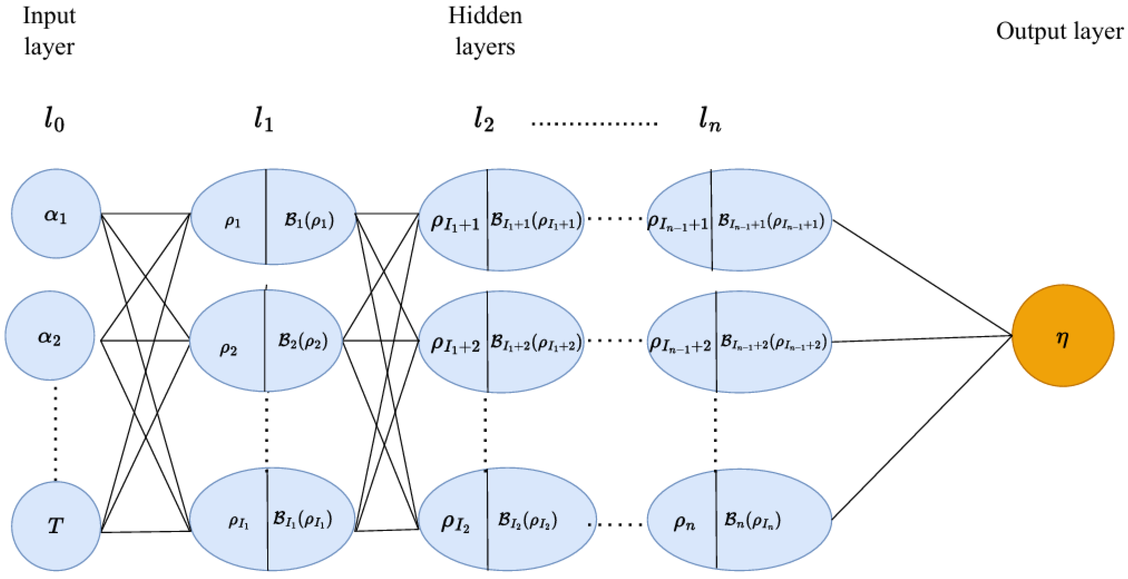
Here, ${\vartheta }_{{\mathcal{I}}_w,\eta }$ denotes the weight connecting the last hidden layer to the output layer, and $\mathcal{B}$ represents the activation function and bias terms $r_{\mathcal{I}}$. For the j-th layer, ${\rho }_{{\mathcal{I}}_y}$ is given by [10]

$${\rho }_{{\mathcal{I}}_y}=r_{{\mathcal{I}}_y}+{\vartheta }_{{\mathcal{I}}_{y-1},{\mathcal{I}}_y}{\mathcal{B}}_{{\mathcal{I}}_{y-1}}({\rho }_{{\mathcal{I}}_{y-1}}),y=1,2,3,4,....,w.$$

(9)

The theory of neural networks uses the method of forward propagation to transfer details from the input phase to the output phase. The sum of the weights and activation characteristics of the neurons produces the final result. The underlying neural network model is illustrated well in Figure 1.

2.2. Neural Network Architecture Incorporating the Riccati Subequation

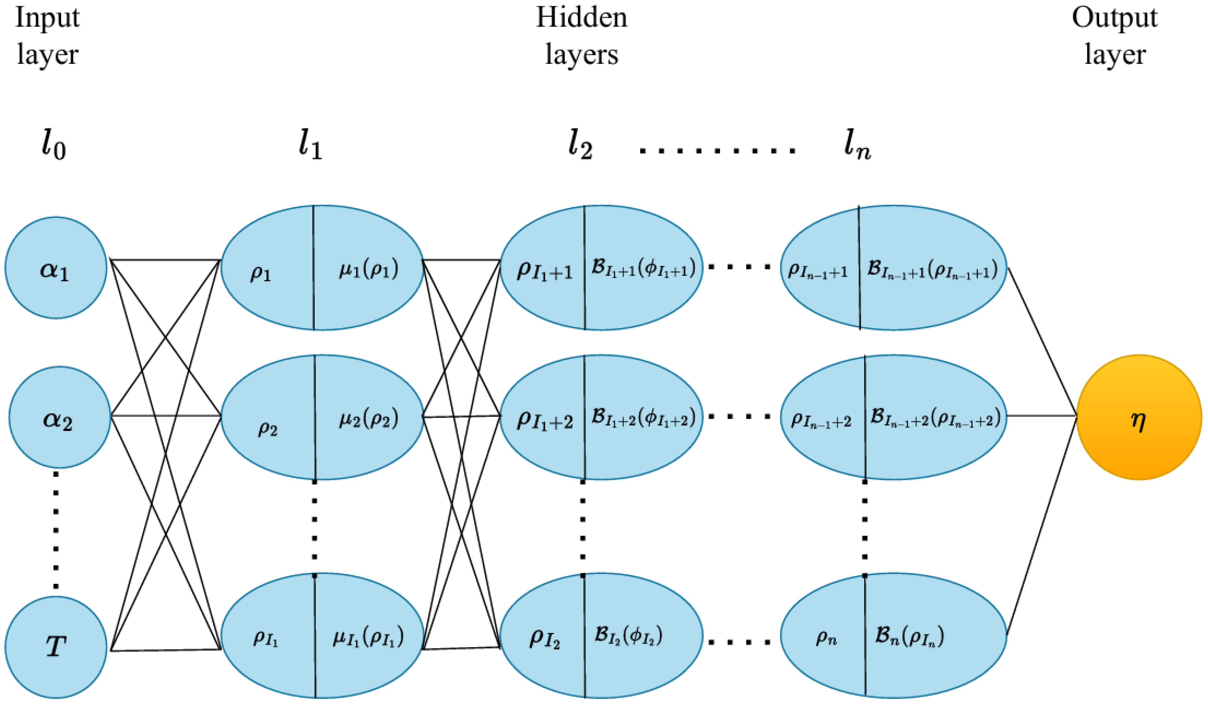
Riccati sub-equation neural networks (RSENNs) form a new hybrid technique that links neural networks with the Riccati sub-equation framework. Their core idea has two pillars [10]:

• Riccati sub-equation solutions are used to select the activation functions for the first hidden layer.
• These activation-based trial functions convert the PDE into algebraic form, enabling new exact solutions.

Step 2: The inital solution of the Riccati sub-equation method is

$${\mu }^{\prime }\left(\eta \right)=\beta +{\mu }^2\left(\eta \right),$$

(10)

The solutions obtained using the Riccati sub-equation method are presented as follows [10]:

• Type 1: When $\beta <0,$

  $$\begin{array}{cc}\hfill & {\mu }_1\left(\eta \right)=-\sqrt{-\beta }tanh\left(\sqrt{-\beta }\eta \right)·\hfill \\ \hfill & {\mu }_2\left(\eta \right)=-\sqrt{-\beta }coth\left(\sqrt{-\beta }\eta \right)·\hfill \\ \hfill & {\mu }_3\left(\eta \right)=-\sqrt{-\beta }tanh\left(2\sqrt{-\beta }\eta \right)\mp \sqrt{-\beta }sech\left(2\sqrt{-\beta }\eta \right).\hfill \\ \hfill & {\mu }_4\left(\eta \right)=-\sqrt{-\beta }coth\left(2\sqrt{-\beta }\eta \right)\mp \sqrt{-\beta }csch\left(2\sqrt{-\beta }\eta \right).\hfill \end{array}$$

  (11)

  $$\begin{array}{cc}\hfill & {\mu }_5\left(\eta \right)=-{\displaystyle \frac{1}{2}}\left(\sqrt{-\beta }tanh\left({\displaystyle \frac{\sqrt{-\beta }}{2}}\eta \right)+\sqrt{-\beta }coth\left({\displaystyle \frac{\sqrt{-\beta }}{2}}\eta \right)\right)·\hfill \\ \hfill & {\mu }_6\left(\eta \right)={\displaystyle \frac{\sqrt{-(h_1^2+h_2^2)\beta }-h_1\sqrt{-\beta }cosh\left(2\sqrt{-\beta }\eta \right)}{h_{1}sinh\left(2\sqrt{-\beta }{\rho }_k\right)+h_2}}.\hfill \\ \hfill & {\mu }_7\left(\eta \right)=-{\displaystyle \frac{\sqrt{-(h_2^2-h_1^2)\beta }-h_1\sqrt{-\beta }sinh\left(2\sqrt{-\beta }\eta \right)}{h_{1}cosh\left(2\sqrt{-\beta }\eta \right)+h_2}}.\hfill \end{array}$$

  (12)
• Type 2: When $\beta >0,$

  $$\begin{array}{cc}\hfill & {\mu }_8\left(\eta \right)=\sqrt{\beta }tan\left(\sqrt{\beta }\eta \right)·\hfill \\ \hfill & {\mu }_9\left(\eta \right)=-\sqrt{\beta }cot\left(\sqrt{\beta }\eta \right)·\hfill \\ \hfill & {\mu }_{10}\left(\eta \right)=-\sqrt{\beta }tan\left(2\sqrt{\beta }\eta \right)\mp \sqrt{\beta }sec\left(2\sqrt{\beta }\eta \right)·\hfill \\ \hfill & {\mu }_{11}\left(\eta \right)=-\sqrt{\beta }cot\left(2\sqrt{\beta }\eta \right)\mp \sqrt{\beta }csc\left(2\sqrt{\beta }\eta \right)·\hfill \\ \hfill & {\mu }_{12}\left(\eta \right)=-{\displaystyle \frac{1}{2}}\left(\sqrt{\beta }tan\left({\displaystyle \frac{\sqrt{\beta }}{2}}\eta \right)+\sqrt{\beta }cot\left({\displaystyle \frac{\sqrt{\beta }}{2}}\eta \right)\right)·\hfill \\ \hfill & {\mu }_{13}\left(\eta \right)={\displaystyle \frac{\mp \sqrt{(h_1^2-h_2^2)\beta }-h_1\sqrt{\beta }cos\left(2\sqrt{\beta }\eta \right)}{h_{1}sin\left(2\sqrt{\beta }\eta \right)+h_2}},h_1,h_2\in \mathcal{W}·\hfill \\ \hfill & {\mu }_{14}\left(\eta \right)={\displaystyle \frac{\mp \sqrt{(h_1^2-h_2^2)\beta }-h_1\sqrt{-\beta }sin\left(2\sqrt{\beta }\eta \right)}{h_{1}cos\left(2\sqrt{\beta }\eta \right)+h_2}},h_1,h_2\in \mathcal{W}.\hfill \end{array}$$

  (13)
• Family 3: When $\beta \ne 0$,

  $${\mu }_{15}\left({\rho }_q\right)={\displaystyle \frac{1}{\eta +h_3}},h_3\in \mathcal{W}.$$

  (14)

2.3. Main Steps of the Approach

1.

Select the Riccati equation using the connection between the first hidden-layer activation functions and the Riccati sub-equation.

2.

Build the RSENN model with activation functions chosen in 1. The model uses inputs $\alpha ,$$\mathcal{T}$ and proceeds through feed-forward computation, as illustrated in Figure 2.

3.

Use the forward-propagation process of RSENNs to obtain the trial functions of the PDE.

4.

Insert these trial functions into the PDE to convert it into algebraic equations.

5.

Solve the resulting algebraic equations by equating coefficients of terms involving $\alpha ,$ and $\mathcal{T}$, or $\mathcal{P}(\alpha ,\mathcal{T})$.

6.

Select the coefficient set that satisfies the system, substitute back into the trial function, and obtain explicit solutions for $\eta$. Equations (11)–(14) then yield exact solutions to Equation (7).

3. Areas of Application

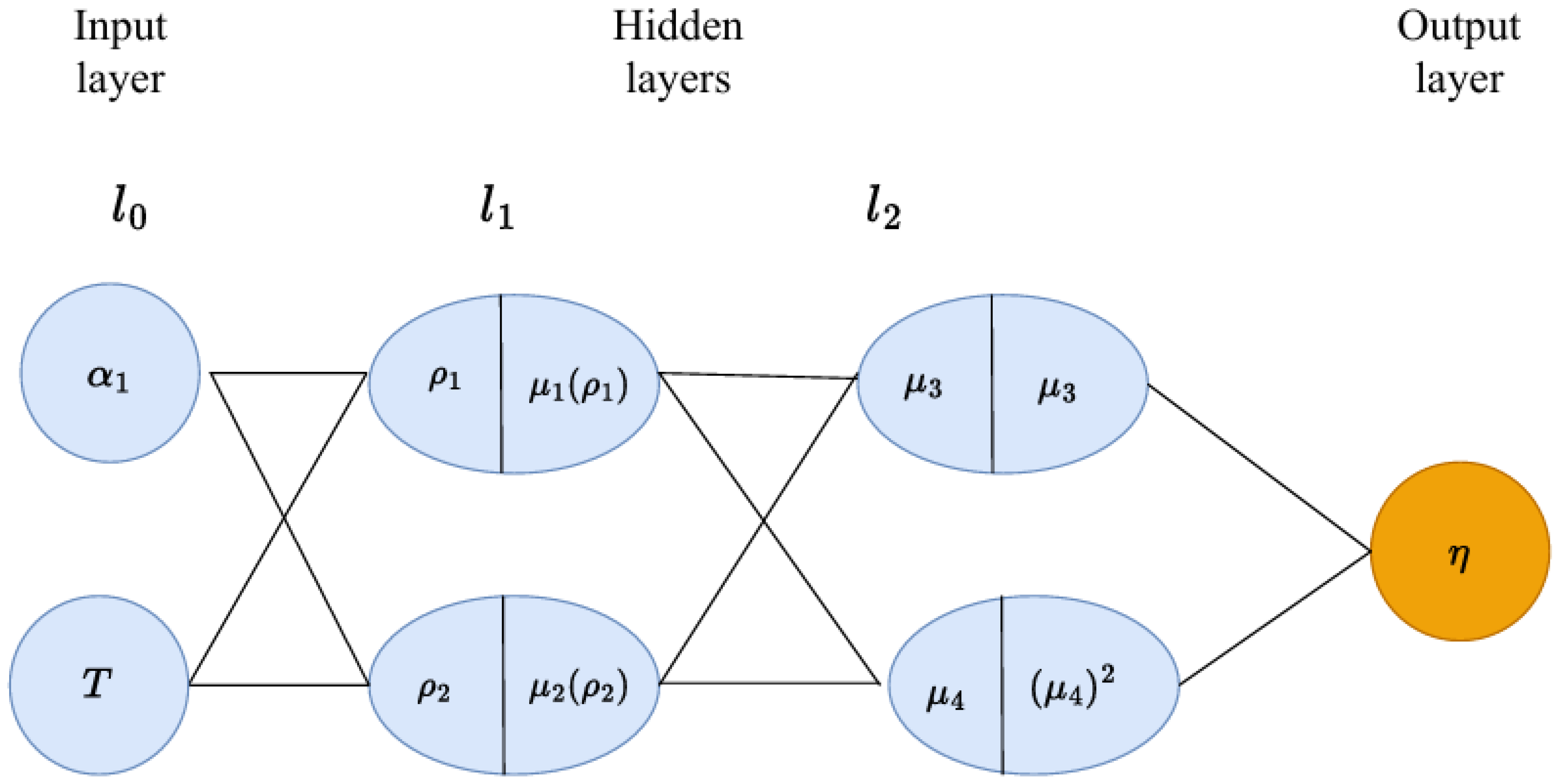
The mBBM equation, an NPDE, is the main topic of this section. To obtain its solutions, we employ the 2-2-2-1 RSENN framework, which consists of three layers—input, hidden, and output—each containing two neurons. Using the trial function $\eta$, the model is utilized to construct approximate solutions for the proposed PDE. We obtain

$$\eta =r_5+{\vartheta }_{3,\eta }{\mathcal{B}}_3\left({\rho }_3\right)+{\vartheta }_{4,\eta }{\mathcal{B}}_4{\left({\rho }_4\right)}^2,$$

(15)

where

$$\begin{array}{cc}\hfill & {\rho }_1=r_1+\mathcal{T}{\vartheta }_{\mathcal{T},1}+\alpha {\vartheta }_{\alpha ,1}\hfill \\ \hfill & {\rho }_2=r_2+\mathcal{T}{\vartheta }_{\mathcal{T},2}+\alpha {\vartheta }_{\alpha ,2}\hfill \\ \hfill & {\rho }_3=r_3+{\vartheta }_{1,3}\mu \left({\rho }_1\right)+{\vartheta }_{1,4}\mu \left({\rho }_2\right)\hfill \\ \hfill & {\rho }_4=r_4+{\vartheta }_{2,3}\mu \left({\rho }_1\right)+{\vartheta }_{2,4}\mu \left({\rho }_2\right)\hfill \end{array}$$

(16)

Here, ${\mu }_y,y=1,2,3,4,$ are the activation functions, $r_{\mathcal{I}},\mathcal{I}=1,2,3,4$ are the bias terms, and ${\vartheta }_{k,j}$ are the trainable parameters to be determined later. We employ the simplified 2-2-2-1 RSENN model, where the first hidden layer uses the Riccati-based activation $\rho (·)$, and the second hidden layer uses the identity and square functions. The inputs are $\alpha$ and $\mathcal{T}$ and the resulting network output is taken as the trial function for the PDE:

$$\eta =r_5+{\vartheta }_{3,\eta }\left({\rho }_3\right)+{\vartheta }_{4,\eta }{\left({\rho }_4\right)}^2,$$

(17)

where

$$\begin{array}{cc}\hfill & {\rho }_1=r_1+\mathcal{T}{\vartheta }_{\mathcal{T},1}+\alpha {\vartheta }_{\alpha ,1}\hfill \\ \hfill & {\rho }_2=r_2+\mathcal{T}{\vartheta }_{\mathcal{T},2}+\alpha {\vartheta }_{\alpha ,2}\hfill \\ \hfill & {\rho }_3=r_3+{\vartheta }_{1,3}\eta \left({\rho }_1\right)+{\vartheta }_{1,4}\eta \left({\rho }_2\right)\hfill \\ \hfill & {\rho }_4=r_4+{\vartheta }_{2,3}\eta \left({\rho }_1\right)+{\vartheta }_{2,4}\eta \left({\rho }_2\right).\hfill \end{array}$$

(18)

Figure 3 illustrates the structure of the 2-2-2-1 RSENN model. For simplicity, we take $r_y=0,y=1,2,3,4$ and set $r_5=r$ during computation. With these adjustments, the expression for the 2-2-2-1 RSENN model becomes

$$\begin{array}{cc}\hfill & \eta ={\vartheta }_{3,\eta }\left({\vartheta }_{1,3}\mu (\mathcal{T}{\vartheta }_{\mathcal{T},1}+\alpha {\vartheta }_{\alpha ,1})+{\vartheta }_{2,3}\mu (\mathcal{T}{\vartheta }_{\mathcal{T},2}+\alpha {\vartheta }_{\alpha ,2})\right)+{\vartheta }_{4,\eta }({\vartheta }_{1,4}\mu (\mathcal{T}{\vartheta }_{\mathcal{T},1}+\alpha {\vartheta }_{\alpha ,1})\hfill \\ & +{\vartheta }_{2,4}\mu (\mathcal{T}{\vartheta }_{\mathcal{T},2}+\alpha {\vartheta }_{\alpha ,2}){)}^2+r.\hfill \end{array}$$

(19)

Here, $\eta$ is the output layer.

Neural Network Study of Equation (6)

We investigate the solutions of Equation (6) using a neural network approach. By substituting Equation (19) into Equation (6) and simplifying the resulting expressions, the solutions are obtained as follows:

• Set 1:

  $$\begin{array}{cc}\hfill & r=0,{\vartheta }_{1,3}={\displaystyle \frac{\mp \sqrt{\frac{6}{2\beta {\mathrm{\Omega }}_0{\vartheta }_{\alpha ,1}^2+{\mathrm{\Omega }}_0}}{\vartheta }_{\alpha ,1}}{{\vartheta }_3}},{\vartheta }_{1,4}={\vartheta }_{2,4}={\vartheta }_{2,3}=0,{\vartheta }_{\mathcal{T},1}=-{\displaystyle \frac{{\vartheta }_{\alpha ,1}}{2\beta {\vartheta }_{\alpha ,1}^2+1}},\hfill \\ & {\vartheta }_{\mathcal{T},2}={\vartheta }_{\mathcal{T},2},{\vartheta }_{\alpha ,1}={\vartheta }_{\alpha ,1},{\vartheta }_{\alpha ,2}={\vartheta }_{\alpha ,2}·\hfill \end{array}$$

  (20)

  The solutions of Equation (6) corresponding to set (20) are given as follows:
• Type 1: When $\beta <0,$

  $$\begin{array}{cc}\hfill & {\mathcal{P}}_{1,1}(\alpha ,\mathcal{T})={\displaystyle \frac{\mp \sqrt{\frac{-6\beta }{2\beta {\mathrm{\Omega }}_0{\vartheta }_{\alpha ,1}^2+{\mathrm{\Omega }}_0}}{\vartheta }_{\alpha ,1}{\vartheta }_{3,\eta }}{{\vartheta }_3}}tanh\left(\sqrt{-\beta }\left(\alpha {\vartheta }_{\alpha ,1}+\mathcal{T}{\vartheta }_{\mathcal{T},1}\right)\right).\hfill \\ \hfill & {\mathcal{P}}_{2,1}(\alpha ,\mathcal{T})={\displaystyle \frac{\mp \sqrt{\frac{-6\beta }{2\beta {\mathrm{\Omega }}_0{\vartheta }_{\alpha ,1}^2+{\mathrm{\Omega }}_0}}{\vartheta }_{\alpha ,1}{\vartheta }_{3,\eta }}{{\vartheta }_3}}coth\left(\sqrt{-\beta }\left(\alpha {\vartheta }_{\alpha ,1}+\mathcal{T}{\vartheta }_{\mathcal{T},1}\right)\right),\hfill \\ \hfill & {\mathcal{P}}_{3,1}(\alpha ,\mathcal{T})={\displaystyle \frac{\mp \sqrt{\frac{-6\beta }{2\beta {\mathrm{\Omega }}_0{\vartheta }_{\alpha ,1}^2+{\mathrm{\Omega }}_0}}{\vartheta }_{\alpha ,1}{\vartheta }_{3,\eta }}{{\vartheta }_3}}(tanh\left(2\sqrt{-\beta }\left(\alpha {\vartheta }_{\alpha ,1}+\mathcal{T}{\vartheta }_{\mathcal{T},1}\right)\right)\mp \mathrm{sech}\left(2\sqrt{-\beta }\left(\alpha {\vartheta }_{\alpha ,1}+\mathcal{T}{\vartheta }_{\mathcal{T},1}\right)\right)).\hfill \\ \hfill & {\mathcal{P}}_{4,1}(\alpha ,\mathcal{T})={\displaystyle \frac{\mp \sqrt{\frac{-6\beta }{2\beta {\mathrm{\Omega }}_0{\vartheta }_{\alpha ,1}^2+{\mathrm{\Omega }}_0}}{\vartheta }_{\alpha ,1}{\vartheta }_{3,\eta }}{{\vartheta }_3}}(coth\left(2\sqrt{-\beta }\left(\alpha {\vartheta }_{\alpha ,1}+\mathcal{T}{\vartheta }_{\mathcal{T},1}\right)\right)\mp \mathrm{csch}\left(2\sqrt{-\beta }\left(\alpha {\vartheta }_{\alpha ,1}+\mathcal{T}{\vartheta }_{\mathcal{T},1}\right)\right)).\hfill \\ \hfill & {\mathcal{P}}_{5,1}(\alpha ,\mathcal{T})={\displaystyle \frac{\mp \sqrt{\frac{-6\beta }{2\beta {\mathrm{\Omega }}_0{\vartheta }_{\alpha ,1}^2+{\mathrm{\Omega }}_0}}{\vartheta }_{\alpha ,1}2{\vartheta }_{3,\eta }}{{\vartheta }_3}}\left(tanh({\displaystyle \frac{\sqrt{-\beta }}{2}}\left(\alpha {\vartheta }_{\alpha ,1}+\mathcal{T}{\vartheta }_{\mathcal{T},1}\right)+coth\left({\displaystyle \frac{\sqrt{-\beta }}{2}}\alpha {\vartheta }_{\alpha ,1}+\mathcal{T}{\vartheta }_{\mathcal{T},1}\right)\right)\hfill \end{array}$$

  (21)

  $$\begin{array}{cc}\hfill & {\mathcal{P}}_{6,1}(\alpha ,\mathcal{T})={\displaystyle \frac{\mp \sqrt{\frac{-6\beta }{2\beta {\mathrm{\Omega }}_0{\vartheta }_{\alpha ,1}^2+{\mathrm{\Omega }}_0}}{\vartheta }_{\alpha ,1}{\vartheta }_{3,\eta }}{{\vartheta }_3}}\left({\displaystyle \frac{\sqrt{-(h_1^2+h_2^2)\beta }-h_1\sqrt{-\beta }cosh\left(2\sqrt{-\beta }\left(\alpha {\vartheta }_{\alpha ,1}+\mathcal{T}{\vartheta }_{\mathcal{T},1}\right)\right)}{h_{1}sinh\left(2\sqrt{-\beta }\left(\alpha {\vartheta }_{\alpha ,1}+\mathcal{T}{\vartheta }_{\mathcal{T},1}\right)\right)+h_2}}\right).\hfill \\ \hfill & {\mathcal{P}}_{7,1}(\alpha ,\mathcal{T})={\displaystyle \frac{\mp \sqrt{\frac{-6\beta }{2\beta {\mathrm{\Omega }}_0{\vartheta }_{\alpha ,1}^2+{\mathrm{\Omega }}_0}}{\vartheta }_{\alpha ,1}{\vartheta }_{3,\eta }}{{\vartheta }_3}}\left({\displaystyle \frac{\sqrt{-(h_2^2-h_1^2)\beta }-h_1\sqrt{-\beta }sinh\left(2\sqrt{-\beta }\left(\alpha {\vartheta }_{\alpha ,1}+\mathcal{T}{\vartheta }_{\mathcal{T},1}\right)\right)}{h_{1}cosh\left(2\sqrt{-\beta }\left(\alpha {\vartheta }_{\alpha ,1}+\mathcal{T}{\vartheta }_{\mathcal{T},1}\right)\right)+h_2}}\right)·\hfill \end{array}$$

  (22)
• Type 2: When $\beta >0,$

  $$\begin{array}{cc}\hfill & {\mathcal{P}}_{8,1}(\alpha ,\mathcal{T})={\displaystyle \frac{\mp \sqrt{\frac{-6\beta }{2\beta {\mathrm{\Omega }}_0{\vartheta }_{\alpha ,1}^2+{\mathrm{\Omega }}_0}}{\vartheta }_{\alpha ,1}{\vartheta }_{3,\eta }}{{\vartheta }_3}}\left(tan\left(\sqrt{\beta }\left(\alpha {\vartheta }_{\alpha ,1}+\mathcal{T}{\vartheta }_{\mathcal{T},1}\right)\right)\right).\hfill \\ \hfill & {\mathcal{P}}_{9,1}(\alpha ,\mathcal{T})={\displaystyle \frac{\mp \sqrt{\frac{-6\beta }{2\beta {\mathrm{\Omega }}_0{\vartheta }_{\alpha ,1}^2+{\mathrm{\Omega }}_0}}{\vartheta }_{\alpha ,1}{\vartheta }_{3,\eta }}{{\vartheta }_3}}\left(cot\left(\sqrt{\beta }\alpha {\vartheta }_{\alpha ,1}+\mathcal{T}{\vartheta }_{\mathcal{T},1}\right)\right).\hfill \\ \hfill & {\mathcal{P}}_{10,1}(\alpha ,\mathcal{T})={\displaystyle \frac{\mp \sqrt{\frac{-6\beta }{2\beta {\mathrm{\Omega }}_0{\vartheta }_{\alpha ,1}^2+{\mathrm{\Omega }}_0}}{\vartheta }_{\alpha ,1}{\vartheta }_{3,\eta }}{{\vartheta }_3}}\left(tan\left(2\sqrt{\beta }\left(\alpha {\vartheta }_{\alpha ,1}+\mathcal{T}{\vartheta }_{\mathcal{T},1}\right)\right)\mp sec\left(2\sqrt{\beta }\left(\alpha {\vartheta }_{\alpha ,1}+\mathcal{T}{\vartheta }_{\mathcal{T},1}\right)\right)\right).\hfill \\ \hfill & {\mathcal{P}}_{11,1}(\alpha ,\mathcal{T})={\displaystyle \frac{\mp \sqrt{\frac{-6\beta }{2\beta {\mathrm{\Omega }}_0{\vartheta }_{\alpha ,1}^2+{\mathrm{\Omega }}_0}}{\vartheta }_{\alpha ,1}{\vartheta }_{3,\eta }}{{\vartheta }_3}}\left(cot\left(2\sqrt{\beta }\left(\alpha {\vartheta }_{\alpha ,1}+\mathcal{T}{\vartheta }_{\mathcal{T},1}\right)\right)\mp csc\left(2\sqrt{\beta }\left(\alpha {\vartheta }_{\alpha ,1}+\mathcal{T}{\vartheta }_{\mathcal{T},1}\right)\right)\right).\hfill \\ \hfill & {\mathcal{P}}_{12,1}(\alpha ,\mathcal{T})={\displaystyle \frac{\mp \sqrt{\frac{-6\beta }{2\beta {\mathrm{\Omega }}_0{\vartheta }_{\alpha ,1}^2+{\mathrm{\Omega }}_0}}{\vartheta }_{\alpha ,1}{\vartheta }_{3,\eta }}{{\vartheta }_3}}\left(tan\left({\displaystyle \frac{\sqrt{\beta }}{2}}\left(\alpha {\vartheta }_{\alpha ,1}+\mathcal{T}{\vartheta }_{\mathcal{T},1}\right)\right)+cot\left({\displaystyle \frac{\sqrt{\beta }}{2}}\left(\alpha {\vartheta }_{\alpha ,1}+\mathcal{T}{\vartheta }_{\mathcal{T},1}\right)\right)\right).\hfill \\ \hfill & {\mathcal{P}}_{13,1}(\alpha ,\mathcal{T})={\displaystyle \frac{\mp \sqrt{\frac{-6\beta }{2\beta {\mathrm{\Omega }}_0{\vartheta }_{\alpha ,1}^2+{\mathrm{\Omega }}_0}}{\vartheta }_{\alpha ,1}{\vartheta }_{3,\eta }}{{\vartheta }_3}}\left({\displaystyle \frac{\mp \sqrt{(h_1^2-h_2^2)}-h_{1}cos\left(2\sqrt{\beta }\left(\alpha {\vartheta }_{\alpha ,1}+\mathcal{T}{\vartheta }_{\mathcal{T},1}\right)\right)}{h_{1}sin\left(2\sqrt{\beta }\left(\alpha {\vartheta }_{\alpha ,1}+\mathcal{T}{\vartheta }_{\mathcal{T},1}\right)\right)+h_2}}\right).\hfill \\ \hfill & {\mathcal{P}}_{14,1}(\alpha ,\mathcal{T})={\displaystyle \frac{\mp \sqrt{\frac{-6\beta }{2\beta {\mathrm{\Omega }}_0{\vartheta }_{\alpha ,1}^2+{\mathrm{\Omega }}_0}}{\vartheta }_{\alpha ,1}{\vartheta }_{3,\eta }}{{\vartheta }_3}}\left({\displaystyle \frac{\mp \sqrt{(h_1^2-h_2^2)}-h_{1}sin\left(2\sqrt{\beta }\left(\alpha {\vartheta }_{\alpha ,1}+\mathcal{T}{\vartheta }_{\mathcal{T},1}\right)\right)}{h_{1}cos\left(2\sqrt{\beta }\left(\alpha {\vartheta }_{\alpha ,1}+\mathcal{T}{\vartheta }_{\mathcal{T},1}\right)\right)+h_2}}\right).\hfill \end{array}$$

  (23)
• Family 3: When $\beta \ne 0$,

  $${\mathcal{P}}_{15,1}(\alpha ,\mathcal{T})={\displaystyle \frac{\mp \sqrt{\frac{-6\beta }{2\beta {\mathrm{\Omega }}_0{\vartheta }_{\alpha ,1}^2+{\mathrm{\Omega }}_0}}{\vartheta }_{\alpha ,1}{\vartheta }_{3,\eta }}{{\vartheta }_3}}\left(\alpha {\vartheta }_{\alpha ,1}+\mathcal{T}{\vartheta }_{\mathcal{T},1}\right)+h_3,h_3\in \mathcal{W}·$$

  (24)
• Set 2:

  $$\begin{array}{cc}\hfill & r=0,{\vartheta }_{2,3}={\displaystyle \frac{\mp \sqrt{\frac{6}{2\beta {\mathrm{\Omega }}_0{\vartheta }_{\alpha ,2}^2+{\mathrm{\Omega }}_0}}{\vartheta }_{\alpha ,2}}{{\vartheta }_3}},{\vartheta }_{1,4}={\vartheta }_{2,4}={\vartheta }_{1,3}=0,{\vartheta }_{\mathcal{T},1}={\vartheta }_{\mathcal{T},1},\hfill \\ & {\vartheta }_{\mathcal{T},2}=-{\displaystyle \frac{{\vartheta }_{\alpha ,2}}{2\beta {\vartheta }_{\alpha ,2}^2+1}},{\vartheta }_{\alpha ,1}={\vartheta }_{\alpha ,1},{\vartheta }_{\alpha ,2}={\vartheta }_{\alpha ,2}·\hfill \end{array}$$

  (25)

  The solutions of Equation (6) corresponding to set (25) are given as follows:
• Type 1: When $\beta <0,$

  $$\begin{array}{cc}\hfill & {\mathcal{P}}_{1,2}(\alpha ,\mathcal{T})={\displaystyle \frac{\mp \sqrt{\frac{-6\beta }{2\beta {\mathrm{\Omega }}_0{\vartheta }_{\alpha ,2}^2+{\mathrm{\Omega }}_0}}{\vartheta }_{\alpha ,2}{\vartheta }_{3,\eta }}{{\vartheta }_3}}(tanh\left(\sqrt{-\beta }\left(\alpha {\vartheta }_{\alpha ,2}+\mathcal{T}{\vartheta }_{\mathcal{T},2}\right)\right)).\hfill \\ \hfill & {\mathcal{P}}_{2,2}(\alpha ,\mathcal{T})={\displaystyle \frac{\mp \sqrt{\frac{-6\beta }{2\beta {\mathrm{\Omega }}_0{\vartheta }_{\alpha ,2}^2+{\mathrm{\Omega }}_0}}{\vartheta }_{\alpha ,2}{\vartheta }_{3,\eta }}{{\vartheta }_3}}(coth\left(\sqrt{-\beta }\left(\alpha {\vartheta }_{\alpha ,2}+\mathcal{T}{\vartheta }_{\mathcal{T},2}\right)\right)).\hfill \\ \hfill & {\mathcal{P}}_{3,2}(\alpha ,\mathcal{T})={\displaystyle \frac{\mp \sqrt{\frac{-6\beta }{2\beta {\mathrm{\Omega }}_0{\vartheta }_{\alpha ,2}^2+{\mathrm{\Omega }}_0}}{\vartheta }_{\alpha ,2}{\vartheta }_{3,\eta }}{{\vartheta }_3}}\left(tanh\left(2\sqrt{-\beta }\left(\alpha {\vartheta }_{\alpha ,2}+\mathcal{T}{\vartheta }_{\mathcal{T},2}\right)\right)\mp \mathrm{sech}\left(2\sqrt{-\beta }\left(\alpha {\vartheta }_{\alpha ,2}+\mathcal{T}{\vartheta }_{\mathcal{T},2}\right)\right)\right).\hfill \end{array}$$

  (26)

  $$\begin{array}{cc}\hfill & {\mathcal{P}}_{4,2}(\alpha ,\mathcal{T})={\displaystyle \frac{\mp \sqrt{\frac{-6\beta }{2\beta {\mathrm{\Omega }}_0{\vartheta }_{\alpha ,2}^2+{\mathrm{\Omega }}_0}}{\vartheta }_{\alpha ,2}{\vartheta }_{3,\eta }}{{\vartheta }_3}}\left(coth\left(2\sqrt{-\beta }\left(\alpha {\vartheta }_{\alpha ,2}+\mathcal{T}{\vartheta }_{\mathcal{T},2}\right)\right)\mp \mathrm{csch}\left(2\sqrt{-\beta }\left(\alpha {\vartheta }_{\alpha ,2}+\mathcal{T}{\vartheta }_{\mathcal{T},2}\right)\right)\right).\hfill \\ \hfill & {\mathcal{P}}_{5,2}(\alpha ,\mathcal{T})={\displaystyle \frac{\mp \sqrt{\frac{-6\beta }{2\beta {\mathrm{\Omega }}_0{\vartheta }_{\alpha ,2}^2+{\mathrm{\Omega }}_0}}{\vartheta }_{\alpha ,2}{\vartheta }_{3,\eta }}{2{\vartheta }_3}}\left(\sqrt{-\beta }tanh\left({\displaystyle \frac{\sqrt{-\beta }}{2}}\left(\alpha {\vartheta }_{\alpha ,2}+\mathcal{T}{\vartheta }_{\mathcal{T},2}\right)\right)+coth\left({\displaystyle \frac{\sqrt{-\beta }}{2}}\left(\alpha {\vartheta }_{\alpha ,2}+\mathcal{T}{\vartheta }_{\mathcal{T},2}\right)\right)\right)).\hfill \\ \hfill & {\mathcal{P}}_{6,2}(\alpha ,\mathcal{T})={\displaystyle \frac{\mp \sqrt{\frac{-6\beta }{2\beta {\mathrm{\Omega }}_0{\vartheta }_{\alpha ,2}^2+{\mathrm{\Omega }}_0}}{\vartheta }_{\alpha ,2}{\vartheta }_{3,\eta }}{{\vartheta }_3}}\left({\displaystyle \frac{\sqrt{-(h_1^2+h_2^2)\beta }-h_1\sqrt{-\beta }cosh\left(2\sqrt{-\beta }\left(\alpha {\vartheta }_{\alpha ,2}+\mathcal{T}{\vartheta }_{\mathcal{T},2}\right)\right)}{h_{1}sinh\left(2\sqrt{-\beta }\left(\alpha {\vartheta }_{\alpha ,2}+\mathcal{T}{\vartheta }_{\mathcal{T},2}\right)\right)+h_2}}\right)·\hfill \\ \hfill & {\mathcal{P}}_{7,2}(\alpha ,\mathcal{T})={\displaystyle \frac{\mp \sqrt{\frac{-6\beta }{2\beta {\mathrm{\Omega }}_0{\vartheta }_{\alpha ,2}^2+{\mathrm{\Omega }}_0}}{\vartheta }_{\alpha ,2}{\vartheta }_{3,\eta }}{{\vartheta }_3}}\left({\displaystyle \frac{\sqrt{-(h_2^2-h_1^2)\beta }-h_1\sqrt{-\beta }sinh\left(2\sqrt{-\beta }\left(\alpha {\vartheta }_{\alpha ,2}+\mathcal{T}{\vartheta }_{\mathcal{T},2}\right)\right)}{h_{1}cosh\left(2\sqrt{-\beta }\left(\alpha {\vartheta }_{\alpha ,2}+\mathcal{T}{\vartheta }_{\mathcal{T},2}\right)\right)+h_2}}\right).\hfill \end{array}$$

  (27)
• Type 2: When $\beta >0,$

  $$\begin{array}{cc}\hfill & {\mathcal{P}}_{8,2}(\alpha ,\mathcal{T})={\displaystyle \frac{\mp \sqrt{\frac{6\beta }{2\beta {\mathrm{\Omega }}_0{\vartheta }_{\alpha ,2}^2+{\mathrm{\Omega }}_0}}{\vartheta }_{\alpha ,2}{\vartheta }_{3,\eta }}{{\vartheta }_3}}\left(tan\left(\sqrt{\beta }\left(\alpha {\vartheta }_{\alpha ,2}+\mathcal{T}{\vartheta }_{\mathcal{T},2}\right)\right)\right)·\hfill \\ \hfill & {\mathcal{P}}_{9,2}(\alpha ,\mathcal{T})={\displaystyle \frac{\mp \sqrt{\frac{6\beta }{2\beta {\mathrm{\Omega }}_0{\vartheta }_{\alpha ,2}^2+{\mathrm{\Omega }}_0}}{\vartheta }_{\alpha ,2}{\vartheta }_{3,\eta }}{{\vartheta }_3}}\left(cot(\sqrt{\beta }\left(\alpha {\vartheta }_{\alpha ,2}+\mathcal{T}{\vartheta }_{\mathcal{T},2}\right)\right)·\hfill \\ \hfill & {\mathcal{P}}_{10,2}(\alpha ,\mathcal{T})={\displaystyle \frac{\mp \sqrt{\frac{6\beta }{2\beta {\mathrm{\Omega }}_0{\vartheta }_{\alpha ,2}^2+{\mathrm{\Omega }}_0}}{\vartheta }_{\alpha ,2}{\vartheta }_{3,\eta }}{{\vartheta }_3}}\left(tan\left(2\sqrt{\beta }\left(\alpha {\vartheta }_{\alpha ,2}+\mathcal{T}{\vartheta }_{\mathcal{T},2}\right)\right)\mp sec\left(2\sqrt{\beta }\left(\alpha {\vartheta }_{\alpha ,2}+\mathcal{T}{\vartheta }_{\mathcal{T},2}\right)\right)\right).\hfill \\ \hfill & {\mathcal{P}}_{11,2}(\alpha ,\mathcal{T})={\displaystyle \frac{\mp \sqrt{\frac{6\beta }{2\beta {\mathrm{\Omega }}_0{\vartheta }_{\alpha ,2}^2+{\mathrm{\Omega }}_0}}{\vartheta }_{\alpha ,2}{\vartheta }_{3,\eta }}{{\vartheta }_3}}\left(cot\left(2\sqrt{\beta }\left(\alpha {\vartheta }_{\alpha ,2}+\mathcal{T}{\vartheta }_{\mathcal{T},2}\right)\right)\mp csc\left(2\sqrt{\beta }\left(\alpha {\vartheta }_{\alpha ,2}+\mathcal{T}{\vartheta }_{\mathcal{T},2}\right)\right)\right).\hfill \\ \hfill & {\mathcal{P}}_{12,2}(\alpha ,\mathcal{T})={\displaystyle \frac{\mp \sqrt{\frac{6\beta }{2\beta {\mathrm{\Omega }}_0{\vartheta }_{\alpha ,2}^2+{\mathrm{\Omega }}_0}}{\vartheta }_{\alpha ,2}{\vartheta }_{3,\eta }}{2{\vartheta }_3}}\left(tan\left({\displaystyle \frac{\sqrt{\beta }}{2}}\left(\alpha {\vartheta }_{\alpha ,2}+\mathcal{T}{\vartheta }_{\mathcal{T},2}\right)\right)+cot\left({\displaystyle \frac{\sqrt{\beta }}{2}}\left(\alpha {\vartheta }_{\alpha ,2}+\mathcal{T}{\vartheta }_{\mathcal{T},2}\right)\right)\right).\hfill \\ \hfill & {\mathcal{P}}_{13,2}(\alpha ,\mathcal{T})={\displaystyle \frac{\mp \sqrt{\frac{6\beta }{2\beta {\mathrm{\Omega }}_0{\vartheta }_{\alpha ,2}^2+{\mathrm{\Omega }}_0}}{\vartheta }_{\alpha ,2}{\vartheta }_{3,\eta }}{{\vartheta }_3}}\left({\displaystyle \frac{\mp \sqrt{(h_1^2-h_2^2)}-h_{1}cos\left(2\sqrt{\beta }\left(\alpha {\vartheta }_{\alpha ,2}+\mathcal{T}{\vartheta }_{\mathcal{T},2}\right)\right)}{h_{1}sin\left(2\sqrt{\beta }\left(\alpha {\vartheta }_{\alpha ,2}+\mathcal{T}{\vartheta }_{\mathcal{T},2}\right)\right)+h_2}}\right),\hfill \\ \hfill & {\mathcal{P}}_{14,2}(\alpha ,\mathcal{T})={\displaystyle \frac{\mp \sqrt{\frac{6\beta }{2\beta {\mathrm{\Omega }}_0{\vartheta }_{\alpha ,2}^2+{\mathrm{\Omega }}_0}}{\vartheta }_{\alpha ,2}{\vartheta }_{3,\eta }}{{\vartheta }_3}}\left({\displaystyle \frac{\mp \sqrt{(h_1^2-h_2^2)}-h_{1}sin\left(2\sqrt{\beta }\left(\alpha {\vartheta }_{\alpha ,2}+\mathcal{T}{\vartheta }_{\mathcal{T},2}\right)\right)}{h_{1}cos\left(2\sqrt{\beta }\left(\alpha {\vartheta }_{\alpha ,2}+\mathcal{T}{\vartheta }_{\mathcal{T},2}\right)\right)+h_2}}\right).\hfill \end{array}$$

  (28)
• Family 3: When $\beta \ne 0$,

  $${\mathcal{P}}_{15,2}(\alpha ,\mathcal{T})={\displaystyle \frac{\mp \sqrt{\frac{6}{2\beta {\mathrm{\Omega }}_0{\vartheta }_{\alpha ,2}^2+{\mathrm{\Omega }}_0}}{\vartheta }_{\alpha ,2}{\vartheta }_{3,\eta }}{{\vartheta }_3\left(\alpha {\vartheta }_{\alpha ,2}+\mathcal{T}{\vartheta }_{\mathcal{T},2}\right)+h_3}},h_3\in \mathcal{W}.$$

  (29)

4. Interpretation of Solution

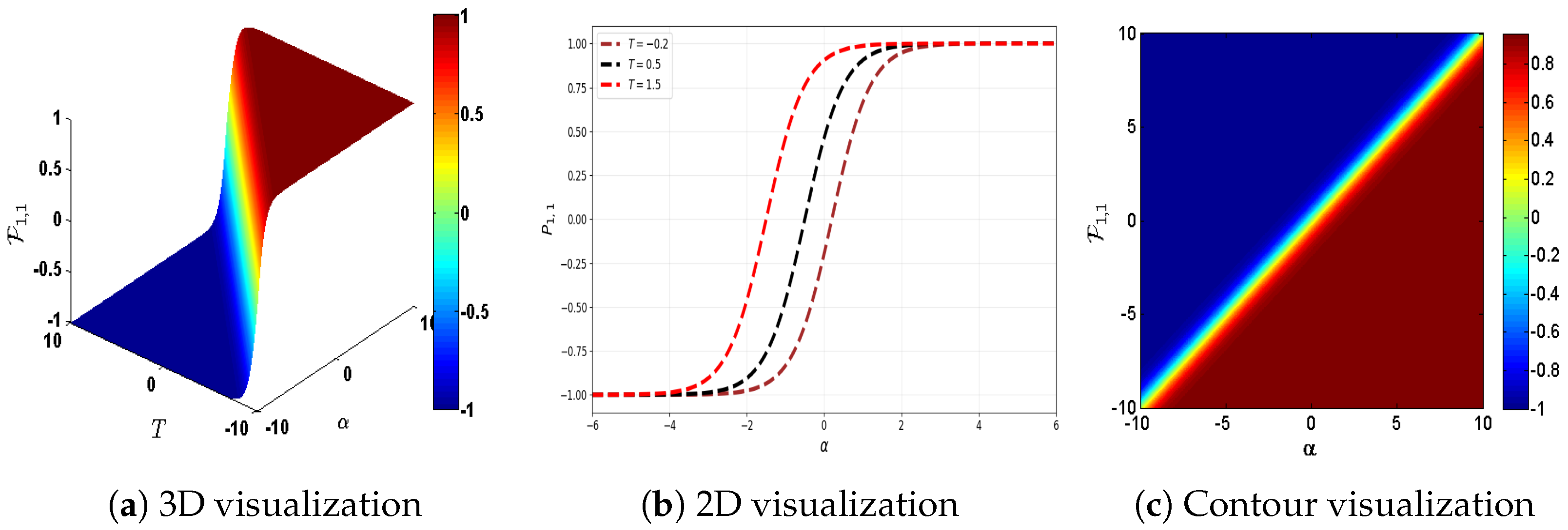
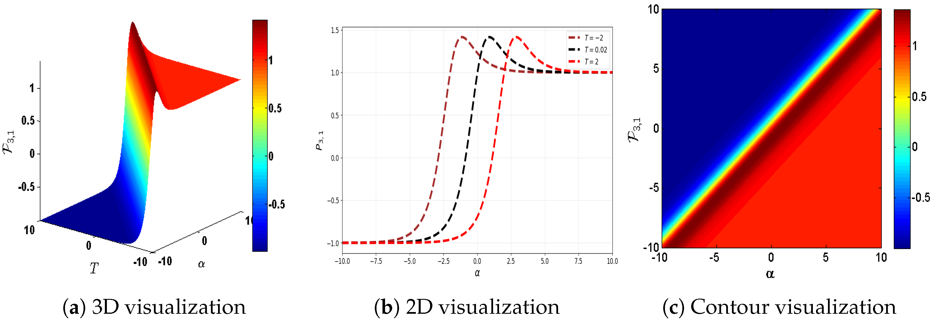
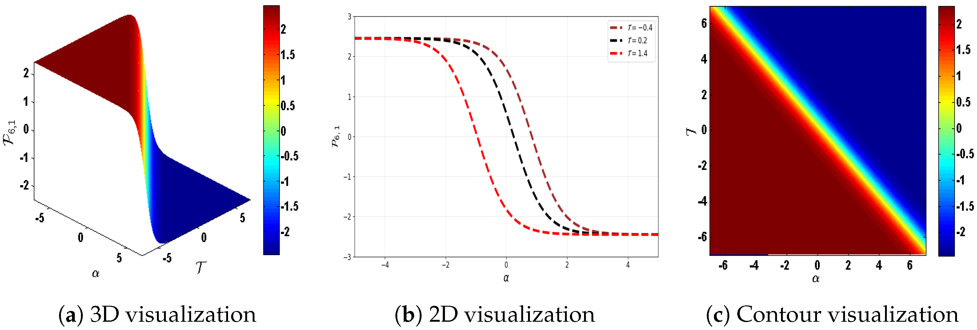
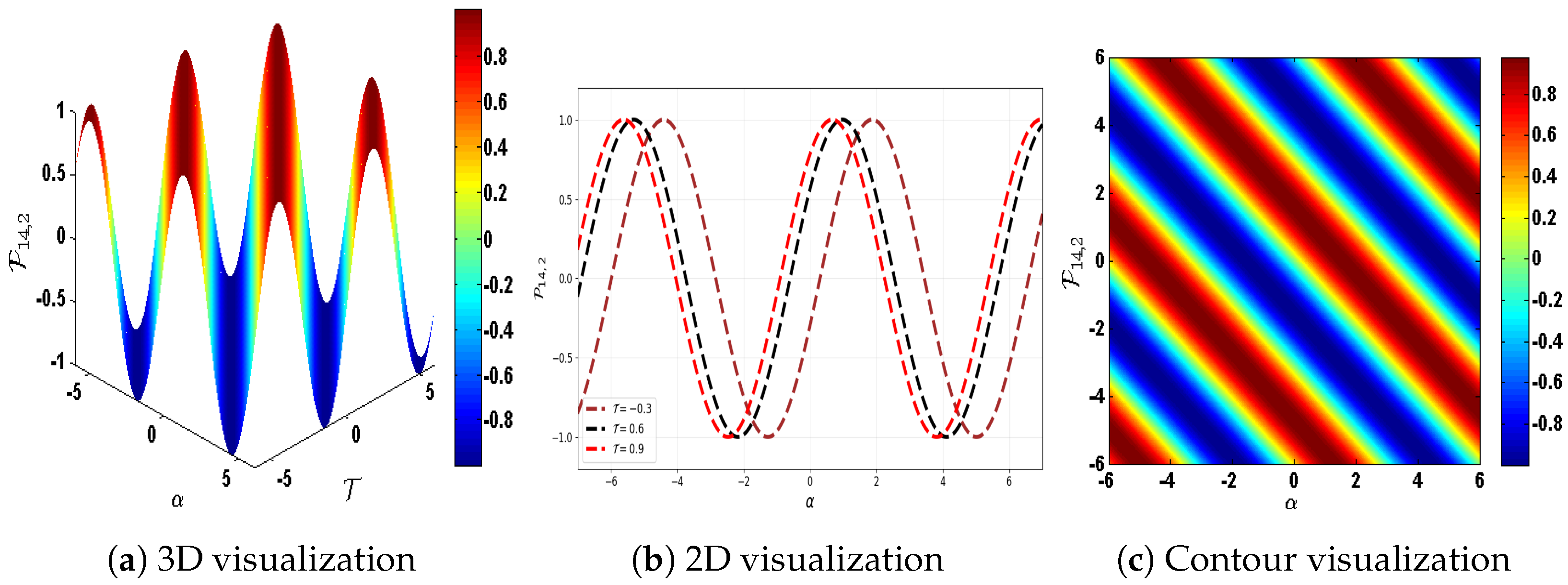
In this section, the graphical characteristics of the solutions ${\mathcal{P}}_{1,1}$, ${\mathcal{P}}_{3,1}$, ${\mathcal{P}}_{6,1}$, and ${\mathcal{P}}_{14,2}$ are investigated through three-dimensional, two-dimensional, and contour plots. Different values of $\beta$ are considered to examine the corresponding wave structures and assess the influence of wave speed on their propagation dynamics. Figure 4 depicts the solution ${\mathcal{P}}_{1,1}$ for the parameter values $\beta =-1.33$, ${\vartheta }_{3,\eta }=1.23$, ${\omega }_0=0.34$, ${\vartheta }_{\alpha ,1}=0.23$, ${\vartheta }_{\mathcal{T},1}=0.13$, and ${\vartheta }_3=1.23$. Under these parameter settings, the solution exhibits a kink-type soliton propagating with a positive wave speed of $0.13$. Figure 5 presents the solution ${\mathcal{P}}_{3,1}$ for $\beta =-1.33$, ${\vartheta }_{3,\eta }=0.33$, ${\omega }_0=0.04$, ${\vartheta }_{\alpha ,1}=0.13$, ${\vartheta }_{\mathcal{T},1}=0.83$, and ${\vartheta }_3=1.23$. The resulting waveform represents a distinct kink-type soliton traveling in the positive direction with a wave speed of $0.43$. The kink soliton model smooths transitions between two stable states, with applications in optical switching and magnetic domain walls. Figure 6 displays the anti-solution ${\mathcal{P}}_{6,1}$ using $\beta =-1.33$, ${\vartheta }_{3,\eta }=0.11$, ${\omega }_0=0.54$, ${\vartheta }_{\alpha ,1}=0.73$, ${\vartheta }_{\mathcal{T},1}=1.23$, and ${\vartheta }_3=1.63$. The corresponding profile takes the form of an anti-kink soliton propagating with a positive wave speed of $1.23$. Anti-kink solitons describe the reverse transition between stable states and are useful in signal reversal and domain-wall dynamics. Figure 7 demonstrates the periodic soliton solution ${\mathcal{P}}_{14,2}$ using $\beta =2.33$, ${\vartheta }_{3,\eta }=0.71$, ${\omega }_0=1.24$, ${\vartheta }_{\alpha ,1}=0.93$, ${\vartheta }_{\mathcal{T},1}=4.23$, and ${\vartheta }_3=1.63$. For this parameter configuration, the solution develops a periodic wave profile that propagates with a positive wave speed of $4.23$. Periodic solitons represent repeating nonlinear wave patterns and are applied in optical communication, plasma physics, and fluid dynamics.

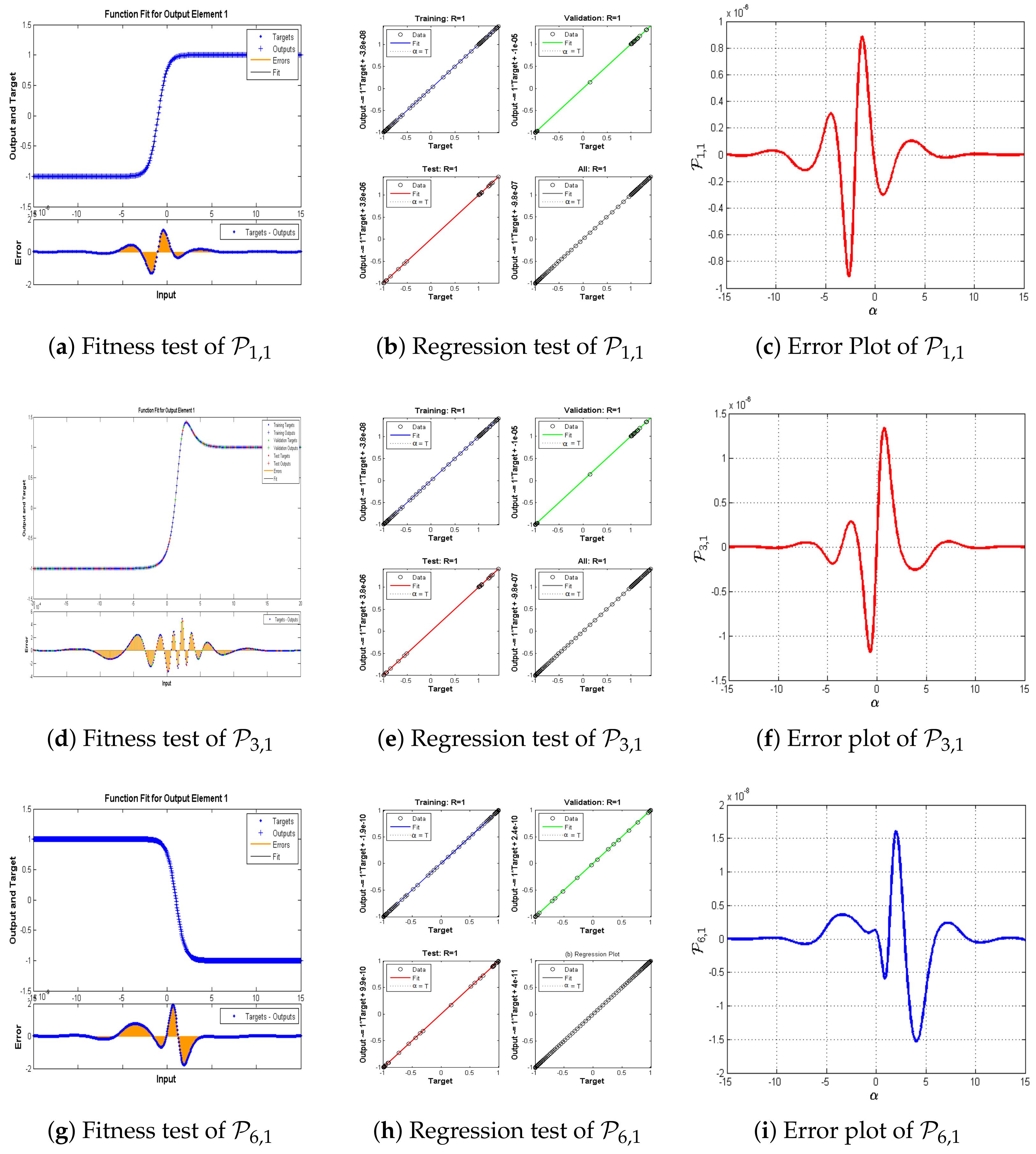
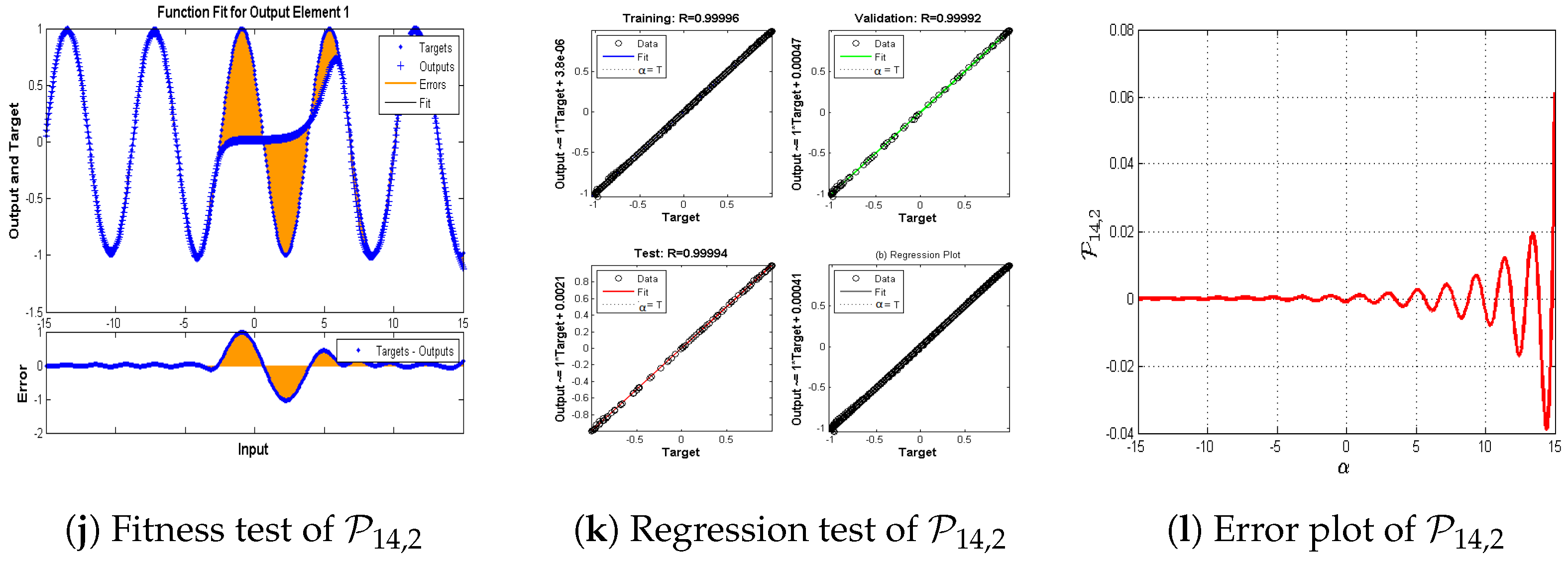
In the second phase, a dataset consisting of 400 points is generated for each variable $\alpha$ and $\mathcal{T}$ within the specified domains $-15\le \alpha \le 15$ and $-16\le \mathcal{T}\le 16$. These data are presented in

Table 3. LM-ANN approximation and generalization performance.

Figure	Training MSE	Validation MSE	Testing MSE	Performance	Gradient	Epochs	Time
Figure 4a–c	3.03300 × ${10}^{-10}$	3.32727 × ${10}^{-10}$	2.76581 × ${10}^{-10}$	7.28 × ${10}^{-14}$	8.98 × ${10}^{-8}$	189	20 s
Figure 5a–c	4.03300 × ${10}^{-10}$	4.23727 × ${10}^{-10}$	3.76581 × ${10}^{-10}$	6.28 × ${10}^{-14}$	7.98 × ${10}^{-8}$	489	26 s
Figure 6a–c	6.07288 × ${10}^{-12}$	5.22439 × ${10}^{-12}$	6.61426 × ${10}^{-12}$	6.07 × ${10}^{-12}$	4.71 × ${10}^{-6}$	990	15 s
Figure 7a–c	4.15676 × ${10}^{-10}$	5.43658 × ${10}^{-10}$	4.34914 × ${10}^{-10}$	6.48 × ${10}^{-6}$	8.47 × ${10}^{-7}$	375	28 s

, corresponding to the solutions ${\mathcal{P}}_{1,1}$, ${\mathcal{P}}_{3,1}$, ${\mathcal{P}}_{6,1}$, and ${\mathcal{P}}_{14,2}$, respectively. In these tables, the variation of $\alpha$ is examined while keeping $\mathcal{T}$ fixed at $\mathcal{T}=2.3$. The constructed datasets are then imported into MATLAB R2018 to implement the proposed LM-ANN model. Furthermore, the dataset is randomly partitioned into three subsets: 75% for training, 15% for validation, and the remaining 10% for testing, as illustrated in Figure 8. This partitioning improves the accuracy, stability, and generalization capability of the model while reducing overfitting and enhancing prediction performance. The LM-ANN model is learned from the data created by the known analytical solutions. Accordingly, training, validation, and testing should be conducted on the following: Errors to quantify the approximation error and generalization ability.

The network performs well over the domain of interest, with a small MSE. The LM-ANN can, as illustrated by the values and good regression results, to exactly capture the analytical soliton shapes. However, these results must not be considered to be a measure of the mathematical stability of the Lyapunov sense, spectral sense, or orbital sense. A rigorous mathematical stability analysis would require a perturbation analysis of the exact solution and an investigation of the range of the corresponding linearized operator.Hence, the present LM-ANN results are used only to evaluate the accuracy of prediction, numerical robustness, and generalization performance.

The proposed RSENN framework is constructed by embedding Riccati sub-equation solutions into the first hidden layer as activation functions. The trial function is derived from the neural network output, where the trainable parameters include weights and biases optimized through the Levenberg–Marquardt algorithm. The Riccati-based activation functions are selected due to their smoothness and ability to represent nonlinear wave structures. The convergence performance is evaluated using training, validation, and testing errors, which demonstrate an accurate approximation of the analytical solutions. The computational complexity mainly depends on the network structure and training iterations; however, the incorporation of analytical information reduces the learning burden compared with conventional neural network approaches.

5. Stability Analysis of the Solution

Stability analysis is used to determine whether the obtained solutions exhibit stable or unstable behavior. In this section, the stability characteristics of the derived solutions are examined by combining the newly developed neural network method with the Hamiltonian approach [32]. The momentum functional corresponding to the Hamiltonian formulation is expressed as

$$\mathcal{F}\left({\vartheta }_{\mathcal{T},1}\right)={\displaystyle \frac{1}{2}}{\int }_{-\infty }^{\infty }\mathcal{P}(\alpha ,\mathcal{T})d\alpha$$

(30)

Stability condition for solution set 1:

$${\displaystyle \frac{\partial \mathcal{F}}{\partial {\vartheta }_{\mathcal{T},1}}}>0.$$

(31)

Stability condition for solution set 2:

$${\displaystyle \frac{\partial \mathcal{F}}{\partial {\vartheta }_{\mathcal{T},2}}}>0.$$

(32)

Here, $\mathcal{F}$ is the momentum and ${\vartheta }_{\mathcal{T},1}$ is the wave speed. If the criterion is satisfied, the solution is stable. Substituting ${\mathcal{P}}_{1,1}$ into Equation (30) and integrating over $\alpha \in [-6,6]$ gives

$$\begin{array}{c}\hfill \mathcal{F}\left({\vartheta }_{\mathcal{T},1}\right)={\displaystyle \frac{\mp {\vartheta }_{3,\eta }}{2{\vartheta }_3\sqrt{-\beta }}}\sqrt{{\displaystyle \frac{-6\beta }{{\mathrm{\Omega }}_0\left(1+2\beta {\vartheta }_{\alpha ,1}^2\right)}}}\times ln\left[{\displaystyle \frac{cosh\left(\sqrt{-\beta }\left(6{\vartheta }_{\alpha ,1}+\mathcal{T}{\vartheta }_{\mathcal{T},1}\right)\right)}{cosh\left(\sqrt{-\beta }\left(\mathcal{T}{\vartheta }_{\mathcal{T},1}-6{\vartheta }_{\alpha ,1}\right)\right)}}\right].\end{array}$$

(33)

To assess the stability criterion, Equation (33) is differentiated with respect to ${\vartheta }_{\mathcal{T},1}$, yielding

$$\begin{array}{cc}\hfill {\displaystyle \frac{\partial \mathcal{F}}{\partial {\vartheta }_{\mathcal{T},1}}}& ={\displaystyle \frac{\mp \mathcal{T}{\vartheta }_{3,\eta }}{2{\vartheta }_3}}\sqrt{{\displaystyle \frac{-6\beta }{{\mathrm{\Omega }}_0\left(1+2\beta {\vartheta }_{\alpha ,1}^2\right)}}}\left[tanh\left(\sqrt{-\beta }\left(6{\vartheta }_{\alpha ,1}+\mathcal{T}{\vartheta }_{\mathcal{T},1}\right)\right)-tanh\left(\sqrt{-\beta }\left(\mathcal{T}{\vartheta }_{\mathcal{T},1}-6{\vartheta }_{\alpha ,1}\right)\right)\right].\hfill \end{array}$$

(34)

For the chosen parameter values, the numerical computation yields

$${\displaystyle \frac{\partial \mathcal{F}}{\partial {\vartheta }_{\mathcal{T},1}}}=0.82614>0.$$

(35)

Since the derivative of the momentum functional with respect to the velocity parameter is positive, the stability criterion for ${\mathcal{P}}_{1,1}$ is satisfied. Hence, the ${\mathcal{P}}_{1,1}$ solution is stable. The stability of the remaining solutions is verified using the same procedure.

6. Conclusions

Neural network frameworks have emerged as powerful tools for solving PDEs, though they often depend on numerical approximations. Hybrid methods now unite neural learning with symbolic computation, achieving exact analytical solutions with greater precision. The sub-equation neural network method computes analytical solutions to the mBBM equation by combining analytical techniques with neural networks. The limitations of conventional analytical approaches can be overcome using the suggested approach. The NLPDE is initially converted for analysis techniques. The results of the suggested techniques are added to the first hidden layer of the neural network model, which uses forward propagation to construct the trial functions. Trial functions are used to set each term’s coefficients to zero. These coefficients can be obtained by solving these algebraic equations. The results are discussed using 3D, 2D, and contour plots, as shown in Figure 4, Figure 5, Figure 6 and Figure 7, to get the kink, anti-kink, and periodic soliton. The accuracy and predictive capability of the Levenberg–Marquardt artificial neural network are assessed by comparing its outputs with the exact analytical solutions, as shown in Figure 8. These approaches have the potential to offer fresh perspectives and an understanding of different NLPDEs, which could help advance numerous scientific fields in the future. By using these methods, researchers can gain a better understanding of how nonlinear systems and events behave.

References

1. Ecke, R.E. Chaos, patterns, coherent structures, and turbulence: Reflections on nonlinear science. Chaos Interdiscip. J. Nonlinear Sci. 2015, 25, 097605. [Google Scholar] [CrossRef] [Scilit]
2. Nicolis, G. Introduction to Nonlinear Science; Cambridge University Press: Cambridge, UK, 1995. [Google Scholar]
3. Alonso, S.; Bär, M.; Echebarria, B. Nonlinear physics of electrical wave propagation in the heart: A review. Rep. Prog. Phys. 2016, 79, 096601. [Google Scholar] [CrossRef] [Scilit]
4. Ming, L.; Muhammad, J.; Yaro, D.; Younas, U. Exploring the multistability, sensitivity, and wave profiles to the fractional Sharma–Tasso–Olver equation in the mathematical physics. AIP Adv. 2025, 15, 045017. [Google Scholar] [CrossRef] [Scilit]
5. Osborne, A.R. Nonlinear ocean wave and the inverse scattering transform. In Scattering; Academic Press: Cambridge, MA, USA, 2002; pp. 637–666. [Google Scholar]
6. Liu, Z.; Zhang, Z.; Lei, Z.; Omura, M.; Wang, R.L.; Gao, S. Dendritic deep learning for medical segmentation. IEEE/CAA J. Autom. Sin. 2024, 11, 803–805. [Google Scholar] [CrossRef] [Scilit]
7. Wang, S.; Zhang, H.; Jiang, X. Physics-informed neural network algorithm for solving forward and inverse problems of variable-order space-fractional advection–diffusion equations. Neurocomputing 2023, 535, 64–82. [Google Scholar] [CrossRef] [Scilit]
8. Liu, Y.; Mao, T.; Zhou, D.X. Approximation of functions from Korobov spaces by shallow neural networks. Inf. Sci. 2024, 670, 120573. [Google Scholar] [CrossRef] [Scilit]
9. Raissi, M.; Perdikaris, P.; Karniadakis, G.E. Physics-informed neural networks: A deep learning framework for solving forward and inverse problems involving nonlinear partial differential equations. J. Comput. Phys. 2019, 378, 686–707. [Google Scholar] [CrossRef] [Scilit]
10. Muhammad, J.; Tipu, G.H.; Alrashedi, Y.; Alhazmi, M.; Younas, U. Analytical study of the nonlinear dynamical systems: Application of the neural networks method. AIMS Math. 2025, 10, 14596–14616. [Google Scholar] [CrossRef] [Scilit]
11. Tipu, G.H.; Cherati, A.Y.; Yao, F.; Momeni, H. Data-driven soliton solutions and parameter discovery to the fourth-order nonlinear AKNS equation: A hybrid analytical and physics-informed neural network approach: G. Hussain Tipu et al. Nonlinear Dyn. 2025, 113, 25047–25069. [Google Scholar]
12. Ming, L.; Muhammad, J.; Yaro, D.; Tipu, G.H.; Younas, U. Investigation of the exact solutions via sub-equation neural network method to the nonlinear systems in fluid and nuclear physics. AIP Adv. 2025, 15, 075208. [Google Scholar] [CrossRef] [Scilit]
13. Islam, M.E.; Khan, K.; Mannaf, M.A.; Akbar, M.A. Diffusion and degradation effect switching closed form solitons to a nonlinear mathematical model. Alex. Eng. J. 2025, 133, 272–283. [Google Scholar] [CrossRef] [Scilit]
14. Muhammad, J.; Bilal, M.; Ur Rehman, S.; Nasreen, N.; Younas, U. Analyzing the decoupled nonlinear Schrödinger equation: Fractional optical wave patterns in the dual-core fibers. J. Opt. 2024, 55, 1257–1268. [Google Scholar] [CrossRef] [Scilit]
15. Wadati, M. The modified Korteweg-de Vries equation. J. Phys. Soc. Jpn. 1973, 34, 1289–1296. [Google Scholar] [CrossRef] [Scilit]
16. Zayed, E.M.; Alngar, M.E.; Shohib, R.; Biswas, A. Highly dispersive solitons in optical couplers with metamaterials having Kerr law of nonlinear refractive index. Ukr. J. Phys. Opt. 2024, 25, 01001–01019. [Google Scholar] [CrossRef] [Scilit]
17. Arnous, A.H. Optical solitons with Biswas–Milovic equation in magneto-optic waveguide having Kudryashov’s law of refractive index. Optik 2021, 247, 167987. [Google Scholar] [CrossRef] [Scilit]
18. Butt, A.R.; Jhangeer, A.; Akgül, A.; Hassani, M.K. A plethora of novel solitary wave solutions related to van der Waals equation: A comparative study. Sci. Rep. 2024, 14, 21665. [Google Scholar] [CrossRef] [Scilit]
19. Kopcasız, B. Unveiling new exact solutions of the complex-coupled Kuralay system using the generalized Riccati equation mapping method. J. Math. Sci. Model. 2024, 7, 146–156. [Google Scholar] [CrossRef] [Scilit]
20. Beenish; Alshammari, F.S. Exploring chaotic behavior, conservation laws, Lie symmetry, and soliton dynamics in the generalized A∓ equation. AIMS Math. 2025, 10, 22150–22179. [Google Scholar] [CrossRef] [Scilit]
21. Beenish; Samreen, M.; Jhangeer, A. Propagation of nonlinear dynamics in atomic chains using chaos theory. Ain Shams Eng. J. 2026, 17, 103828. [Google Scholar] [CrossRef] [Scilit]
22. Alzahrani, T.; Ur Rahman, M. Lump, breathing inelastic collision phenomena, and rogue wave solutions for an extended KP hierarchy-type equation by neural network-based method. Ain Shams Eng. J. 2025, 16, 103657. [Google Scholar] [CrossRef] [Scilit]
23. AL-Essa, L.A.; Ur Rahman, M. Analysis of Lie symmetry, bifurcations with phase portraits, sensitivity, and diverse WM shape soliton solutions for the (2+1)-dimensional evolution equation. Phys. Lett. A 2024, 525, 129928. [Google Scholar] [CrossRef] [Scilit]
24. Shakeel, M.; Manan, A.; Turki, N.B.; Shah, N.A.; Tag, S.M. Novel analytical technique to find a diversity of solitary wave solutions for Wazwaz-Benjamin-Bona Mahony equations of fractional order. Results Phys. 2023, 51, 106671. [Google Scholar] [CrossRef] [Scilit]
25. Shakeel, M.; Turki, N.B.; Shah, N.A.; Tag, S.M. Diversity of soliton solutions to the (3+1)-dimensional Wazwaz-Benjamin-Bona-Mahony equations arising in mathematical physics. Results Phys. 2023, 51, 106624. [Google Scholar] [CrossRef] [Scilit]
26. Akbulut, A.; Islam, S.R.; Rezazadeh, H.; Taşcan, F. Obtaining exact solutions of nonlinear partial differential equations via two different methods. Int. J. Mod. Phys. B 2022, 36, 2250041. [Google Scholar] [CrossRef] [Scilit]
27. Li, W.; Akinyemi, L.; Lu, D.; Khater, M.M. Abundant traveling wave and numerical solutions of weakly dispersive long waves model. Symmetry 2021, 13, 1085. [Google Scholar] [CrossRef] [Scilit]
28. Attia, R.A.M.; Khater, M.M.A. The mBBM equation: A mathematical key to unlocking wave behavior in fluids. Int. J. Math. Comput. Eng. 2024, 3, 171–184. [Google Scholar] [CrossRef] [Scilit]
29. Khater, M.M.; Salama, S.A. Semi-analytical and numerical simulations of the modified Benjamin-Bona-Mahony model. J. Ocean Eng. Sci. 2022, 7, 264–271. [Google Scholar] [CrossRef] [Scilit]
30. Wang, K.J. Variational principle and diverse wave structures of the modified Benjamin-Bona-Mahony equation arising in the optical illusions field. Axioms 2022, 11, 445. [Google Scholar] [CrossRef] [Scilit]
31. Beenish; Samreen, M. Analytical solutions and dynamical insights of the modified Benjamin-Bona-Mahony equation with applications in nonlinear optics. J. Appl. Math. Comput. 2025, 71, 699–723. [Google Scholar] [CrossRef] [Scilit]
32. Razzaq, W.; Zafar, A.; Al Nuaim, A.; Al Nuaim, A. A WAS neural network framework for computing and analyzing solutions of a generalized (3 + 1)-dimensional nonlinear Wave equation: Stability analysis. AIMS Math. 2026, 11, 10694–10715. [Google Scholar] [CrossRef] [Scilit]
Figure 1. NN architecture.
Mca 31 00175 g001
Figure 2. PENN model.
Mca 31 00175 g002
Figure 3. The 2–2–2–1 PENN model of Equation (15).
Mca 31 00175 g003
Figure 4. Kink-type soliton solution of P 1 , 1 ( α , T ) using β = 1.33 , ϑ 3 , η = 1.23 , ω 0 = 0.34 , ϑ α , 1 = 0.23 , ϑ T , 1 = 0.13 , and ϑ 3 = 1.23 .
Mca 31 00175 g004
Figure 5. Second kind of kink solution of P 3 , 1 ( α , T ) using β = 1.33 , ϑ 3 , η = 0.33 , ω 0 = 0.04 , ϑ α , 1 = 0.13 , ϑ T , 1 = 0.83 , and ϑ 3 = 1.23 .
Mca 31 00175 g005
Figure 6. Anti-kink solution of P 6 , 1 ( α , T ) using β = 1.33 , ϑ 3 , η = 0.11 , ω 0 = 0.54 , ϑ α , 1 = 0.73 , ϑ T , 1 = 1.23 , and ϑ 3 = 1.63 .
Mca 31 00175 g006
Figure 7. Periodic soliton solution of P 14 , 2 ( α , T ) using β = 2.33 , ϑ 3 , η = 0.71 , ω 0 = 1.24 , ϑ α , 1 = 0.93 , ϑ T , 1 = 4.23 , and ϑ 3 = 1.63 .
Mca 31 00175 g007
Figure 8. Numerical convergence of the solution using the LM-ANN approach.
Mca 31 00175 g008aMca 31 00175 g008b