Mathematical Modeling for Tumor–Immune Dynamics with Clinical Validation

Abstract

Pituitary adenoma is a clinically important brain tumor whose progression and therapeutic outcomes are influenced by intricate interactions between tumor development and the host immune response. Globally, pituitary adenomas account for approximately 15% of all intracranial tumors. This study aims to investigate clinical MRI data obtained from a patient who recovered from a pituitary adenoma. The collected data provide measurements of tumor volume (mm) at several time points throughout the treatment period. The patient received vaccine-based therapy accompanied by regular clinical assessments, and achieved recovery after nearly twenty-two months. Motivated by the clinical observations and the underlying treatment mechanism, a mathematical model describing tumor–immune–vaccine interactions is developed. The proposed ordinary differential equation (ODE) framework incorporates tumor cells, immune cells, and vaccine components to characterize the temporal evolution of tumor volume during treatment. Fundamental dynamical properties of the model, including positivity, boundedness, existence of solutions, and equilibrium stability, are established through analytical techniques. In addition, numerical simulations are performed using the fourth-order Runge–Kutta (RK4) method and validated against the available clinical measurements. The numerical results exhibit close agreement between the observed and simulated data, yielding a minimal root mean square error (RMSE). Furthermore, sensitivity analysis highlights the significant role of immune- and vaccine-related parameters in regulating tumor suppression. The findings suggest that a relatively simple mechanistic framework can effectively capture the reduction in pituitary adenoma under vaccine-based therapy.

1. Introduction

1.1. Motivation

Although cancer research is progressing at a rapid pace with the implementation of the most recent therapies and techniques, there is still a requirement for instruments that can connect clinically observed data to the biological interaction between the tumor, immune response, and therapeutic effects. MRI data provide a more detailed picture, highlighting abnormalities in soft tissues impacted by tumors and their implications on surrounding tissues. However, it fails to describe the mechanisms behind these changes in detail. Furthermore, most mathematical models focus on generic tumors or theoretical elements of tumor immunological interactions, without taking into account patient-specific clinical observations of pituitary adenoma receiving vaccine-based treatment. These constraints encourage the development of a patent-specific mathematical model that incorporates tumor–immune dynamics and clinical information. The goal of this study is to develop and analyze a patient-specific model aligned with treatment and clinical data.

Cancer is a leading cause of death worldwide, and it is largely acknowledged as one of the most challenging diseases to adequately treat in clinical practice. As a result, cancer therapy remains one of contemporary medicine’s most difficult issues. The fundamental goal of treatment is to eradicate malignant cells while maintaining a sufficient number of healthy cells. Brain tumors are a diverse category of neoplasms affecting the central nervous system (CNS) that continue to cause significant morbidity and mortality around the world [1,2]. Pituitary adenomas, also known as pituitary neuroendocrine tumors (PitNETs), are responsible for 10–15% of all intracranial neoplasms [3]. Although most pituitary adenomas are histologically benign, they can cause significant clinical problems due to hormonal hypersecretion, compression of adjacent structures, visual abnormalities, and tumor recurrence. Their biological behavior varies greatly between patients, making precise assessment of tumor growth and therapy response a major therapeutic problem. 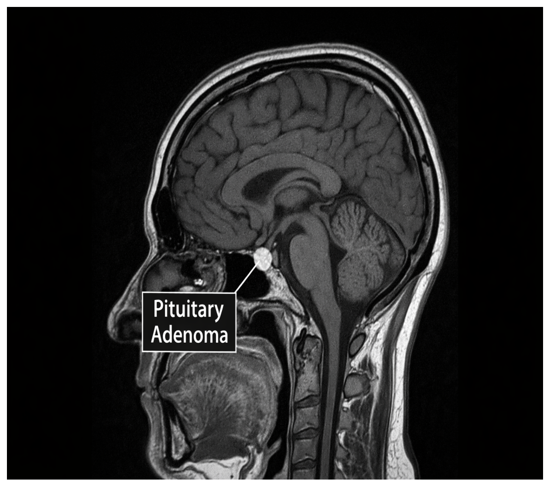Transsphenoidal surgery, medicinal therapy, radiation, and developing immunological techniques are all currently available therapeutic options [4,5]. Pituitary adenomas are tumors found in the anterior pituitary gland (see Figure 1), as highlighted by the authors in [6].

Although these tumors are generally considered benign, they may display aggressive and unpredictable clinical behavior. In recognition of this variability, the European Pituitary Pathology Group (EPPG) has recommended replacing the term “adenoma” with “neuroendocrine pituitary tumor” to better capture their biological complexity [7]. Pituitary adenomas are characterized according to their size and functional status. Microadenomas are tumors with a maximum diameter of less than 10 mm, while macroadenomas have a diameter of 10 mm or more. Giant pituitary adenomas are often tumors with a maximum diameter of 40 mm or greater [8].

Mathematical modeling offers useful insights into disease progression by combining data from several biological scales, such as genetic, cellular, and molecular processes. Through simulation and experimental design, these models aid in the identification of underlying illness mechanisms, the evaluation of new therapeutic options, and the enhancement of drug development efficiency. Furthermore, quantitative modeling promotes personalized medicine by allowing treatment plans to be customized to patient-specific variables such as disease severity and biological variability. Mathematical models have grown in importance in current medical research and healthcare decision-making because they help clinicians predict treatment results and optimize resource allocation [9].

1.2. Related Work

Mathematical modeling has emerged as a valuable tool for analyzing tumor growth and evaluating therapy options. Several studies have employed conventional tumor growth models, such as exponential, logistic, Gompertz, and Bertalanffy formulations, to describe and predict cancer dynamics under various therapeutic approaches [10,11,12,13,14]. These models offer significant insights into tumor progression and treatment response; however, they are frequently built with generic datasets rather than patient-specific clinical data. A second group of investigations looked into vaccine- and immunotherapeutic methods. Mathematical frameworks have been developed to assess anticancer viral vaccines, personalized neoantigen vaccines, combined vaccination and immunotherapy techniques, and dendritic-cell-targeted vaccines [15,16,17,18,19,20]. These studies show that vaccination can increase immune responses while suppressing tumor growth. In parallel, researchers created tumor–immune interaction models utilizing both traditional and innovative mathematical methods. These include delay differential equation models, stochastic formulations, and fractional-order systems that represent the complicated biological interactions between tumor cells and immunological responses [21,22,23,24,25,26]. Such research has improved our understanding of immune-mediated tumor control and therapeutic optimization. Although pituitary tumors have garnered more attention in clinical and computational research, previous investigations have generally focused on hormonal modulation, postoperative outcome prediction, or overall tumor growth [27,28]. Many studies of tumor immune interactions highlighted optimal control strategies to minimize the adverse effects of chemo-immunotherapy and maximize treatment outcomes [29,30,31,32,33]. Notably, studies [34,35,36] have highlighted the stochastic dynamics of cancers. Few studies have developed patient-specific mathematical models of pituitary adenoma progression based on real-world clinical measures and vaccine-based treatment. As a result, there is still a significant research gap in combining clinical MRI-derived tumor data with mechanistic tumor–immune–vaccine dynamics. To fill this gap, the current study develops a patient-specific ODE-based mathematical model of pituitary adenoma growth and regression vaccination treatment. Unlike many other theoretical models, the proposed framework is calibrated and validated with longitudinal clinical measures from a recovered patient. This combination of clinical evidence and mathematical modeling creates a quantitative framework for understanding vaccine-driven tumor suppression and assessing treatment effects.

The novelty of this work is that it presents a patient-specific mathematical model of a pituitary tumor derived directly from MRI data (tumor size) of a patient recovered through vaccine-based treatment. Unlike conventional theoretical tumor models, it integrates real clinical data with immune vaccine interaction to describe suppression of tumor volume. Although many studies provide clinical validation of tumor immune models, most of them deal with generic tumors, which mostly deal with breast cancers, lung cancer, and brain tumors in general, and use large datasets. This case study particularly deals with a pituitary adenoma treated with a vaccine rather than any therapy. To the best of our knowledge, the literature contains a limited number of studies of pituitary adenoma, and lacks studies on a particular patient-specific model aligned with treatment.

In this study, longitudinal clinical data from a patient diagnosed with pituitary adenoma and treated with a vaccine-based therapeutic approach are considered. Motivated by the observed tumor response under treatment, an ordinary differential equation (ODE) model describing tumor–immune–vaccine interactions is developed. The qualitative properties of the proposed model, including positive invariance, boundedness, the existence and uniqueness of solutions, and the stability of equilibrium states, are investigated. Numerical simulations are then performed using the classical fourth-order Runge–Kutta (RK4) method, and the model predictions are compared with clinical observations to assess the ability of the framework to describe tumor progression and regression under treatment.

The manuscript is organized as follows: Section 1 presents the introduction, followed by a review of the related literature. The proposed mathematical framework is developed and described in Section 2. Section 3 is devoted to the qualitative analysis of the model followed by analysis of the stability of the equilibrium states in Section 4. Section 5 provides the results illustrated graphically, along with corresponding interpretation and discussion. Lastly, Section 6 presents concluding remarks, limitations, and potential future directions in this area.

2. Tumor–Immune Vaccine Model

A system of ordinary differential equations (ODEs) describing the interactions among tumor cells, immune cells, and vaccine concentration is proposed and is given by

$$\begin{array}{c}\hfill \begin{array}{c}\hfill \dot{T}\left(t\right)=\alpha T\left(1-{\displaystyle \frac{T}{K}}\right)-\beta IT-\gamma VT,\\ \hfill \dot{I}\left(t\right)=\delta VT+\rho I-\eta I,\\ \hfill \dot{V}\left(t\right)=\mu -eV,\end{array}\end{array}$$

(1)

where $T\left(t\right)$, $I\left(t\right)$, and $V\left(t\right)$ represents tumor cell population, immune cell population and vaccine concentration, respectively. The system possess the following initial conditions: $T\left(0\right)={\tau }_0\ge 0,I\left(0\right)=I_0\ge 0,V\left(0\right)=v_0\ge 0$.

The tumor cell population follows logistic growth expressed by the term $\alpha T(1-{\displaystyle \frac{T}{K}})$, where $\alpha$ represents the intrinsic growth rate of the tumor and K denotes the carrying capacity of tumor cells. The choice of the logistic growth model is determined by a variety of considerations, including biological interpretability, mathematical simplicity, and suitability for parameter estimation based on the limited clinical observations available in the present study. It provides adequate descriptions of tumor dynamics with a small number of parameters. For complex models with a large number of parameters and a dataset, Richard’s model can be an option. The term $-\beta IT$ represents the interaction of immune and tumor cells, where $\beta$ denotes the killing rate of the tumor by immune cells. The tumor growth is impacted by the interaction with the vaccine, denoted by $-\gamma VT$, where $\gamma$ expresses the killing rate of the tumor by the vaccine. In the second equation, $\delta VT$ expresses the tumor–vaccine interaction, and it is taken as positive because it reflects immune enhancement triggered by vaccine–tumor interaction. Although immune cells can be activated by antigen presentation. The current study ignores this assumption. The term $(\rho -\eta )I$ represents the proliferation and the natural death rate of immune cells, respectively. In the third equation, $\mu$ is the concentration of the vaccine and $eV$ expresses the decay rate of the administered drug. A description of the parameters involved in the formulation of model and their physical interpretation are listed below in

Table 1. Parameter descriptions.

Notation	Description	Values	Units
$\alpha$	Growth rate of tumor cells	(0.2–0.65)	${\mathrm{cell}}^{-1}$
$\beta$	Rate of tumor-killing by immune cells	(0.02–0.2)	${\mathrm{cell}}^{-1}$
$\gamma$	Rate of tumor-killing by vaccine	(0.005–0.1)	${\mathrm{cell}}^{-1}$
K	Carrying capacity of tumor cells	(0.25–0.55)	${\mathrm{cell}}^{-1}$
$\delta$	Activation rate of immune cells due to tumor and vaccine	(0.02–0.3)	${\mathrm{cell}}^{-1}$
$\rho$	Proliferation rate of immune cells	(0.05–0.7)	${\mathrm{day}}^{-1}$
$\eta$	Natural death rate of immune cells	(0.01–0.15)	${\mathrm{day}}^{-1}$
$\mu$	Amount of vaccine	(0.5–2.0)	${\mathrm{cell}}^{-1}$
e	Drug decay rate	(0.2–1.0)	${\mathrm{cell}}^{-1}{\mathrm{day}}^{-1}$
T	Tumor volume	$0.113$	mL
I	Immune cell population	$1.0$	million cells
V	Vaccine	$1.5$	mg/mL

.

The parameter ranges provided in Table 1 were chosen from previously published tumor–immune interaction models and then adjusted to remain biologically realistic for pituitary tumor growth and vaccine-induced therapeutic response. Since direct clinical measurements for numerous model parameters are unavailable, ranges rather than fixed values are used to account for patient biological variability, as well as uncertainty associated with immunological and vaccination responses.

2.1. Methodology

The proposed tumor–immune–vaccine model is represented by a system of nonlinear ordinary differential equations describing the temporal evolution of tumor cells $T\left(t\right)$, immune cells $I\left(t\right)$, and vaccine concentration ($V\left(t\right)$). Let

$$\mathbf{Y}={(T,I,V)}^T,\mathrm{then}{\displaystyle \frac{d\mathbf{Y}}{dt}}={\left({\displaystyle \frac{dT}{dt}},{\displaystyle \frac{dI}{dt}},{\displaystyle \frac{dV}{dt}}\right)}^T=\mathbf{F}\left(\mathbf{Y}\right).$$

where

$$\mathbf{F}\left(\mathbf{Y}\right)=\left(\begin{array}{c}\alpha T\left(1-{\displaystyle \frac{T}{K}}\right)-\beta IT-\gamma VT,\\ \delta VT+\rho I-\eta I,\\ -eV+\mu \end{array}\right).$$

$${\displaystyle \frac{d\mathbf{Y}}{dt}}=\mathbf{F}(t,\mathbf{Y}),\mathbf{Y}\left(t_0\right)={\mathbf{Y}}_0={(T_0,I_0,V_0)}^T.$$

The RK4 scheme advances the solution from time $t_n$ to $t_{n+1}=t_n+\Delta t$ as

$${\mathbf{Y}}_{n+1}={\mathbf{Y}}_n+{\displaystyle \frac{\Delta t}{6}}\left({\mathbf{k}}_1+2{\mathbf{k}}_2+2{\mathbf{k}}_3+{\mathbf{k}}_4\right),$$

with

$$\begin{array}{cc}\hfill {\mathbf{k}}_1& =\mathbf{F}(t_n,{\mathbf{Y}}_n),\hfill \\ \hfill {\mathbf{k}}_2& =\mathbf{F}\left(t_n+{\displaystyle \frac{\Delta t}{2}},{\mathbf{Y}}_n+{\displaystyle \frac{\Delta t}{2}}{\mathbf{k}}_1\right),\hfill \\ \hfill {\mathbf{k}}_3& =\mathbf{F}\left(t_n+{\displaystyle \frac{\Delta t}{2}},{\mathbf{Y}}_n+{\displaystyle \frac{\Delta t}{2}}{\mathbf{k}}_2\right),\hfill \\ \hfill {\mathbf{k}}_4& =\mathbf{F}(t_n+\Delta t,{\mathbf{Y}}_n+\Delta t{\mathbf{k}}_3).\hfill \end{array}$$

2.2. Root Mean Square Error (RMSE)

The root mean square error (RMSE) was used to quantify the discrepancy between observed tumor volumes and model predictions [37]. Mathematically,

$$\mathrm{RMSE}=\sqrt{{\displaystyle \frac{1}{n}}{\displaystyle \sum _{i=1}^n}{(T_{o}bs\left(t_i\right)-T_{n}um\left(t_i\right))}^2}.$$

where $T_{o}bs$ represents observed data from B-spline and $T_{n}um$ expresses numerical values from RK4.

Algorithm 1 outlines the implementation of the Fourth-Order Runge–Kutta (RK4) method used to solve the proposed model.

Algorithm 1: Fourth-Order Runge–Kutta (RK4) Method

Require: System of ODEs ${\displaystyle \frac{d\mathbf{Y}}{dt}}=\mathbf{F}(t,\mathbf{Y})$, initial state $\mathbf{Y}\left(0\right)={\mathbf{Y}}_0$, step size $h={\displaystyle \frac{t_f-t_0}{N}}$

Ensure: Approximate solution $\mathbf{Y}\left(t\right) \mathrm{on} [0,22].$

Set initial time $t_0=0 \left(\mathrm{months}\right),$

Set final time $t_f=22 \left(\mathrm{months}\right),$

Compute number of steps $N={\displaystyle \frac{t_f-t_0}{h}},$

Initialize $t=t_0,\mathbf{Y}={\mathbf{Y}}_0,$

for $n=0 \mathrm{to} N-1 \mathbf{do}$

$k_1=\mathbf{F}\left(t_n,{\mathbf{Y}}_n\right),$

$k_2=\mathbf{F}\left(t_n+{\displaystyle \frac{h}{2}},{\mathbf{Y}}_n+{\displaystyle \frac{h}{2}}{k}_1\right),$

$k_3=\mathbf{F}\left(t_n+{\displaystyle \frac{h}{2}},{\mathbf{Y}}_n+{\displaystyle \frac{h}{2}}{k}_2\right),$

$k_4=\mathbf{F}\left(t_n+h,{\mathbf{Y}}_n+h{k}_3\right),$

Update state variable: ${\mathbf{Y}}_{n+1}={\mathbf{Y}}_n+{\displaystyle \frac{h}{6}}\left(k_1+2k_2+2k_3+k_4\right),$

Update time: $t_{n+1}=t_n+h,$

end for

return Numerical approximation $\mathbf{Y}\left(t\right) \mathrm{on} [0,22].$

3. Model Dynamics

This section focuses on qualitative analysis of the model, including positivity, existence, boundedness, and stability of equilibrium states.

3.1. Positive Invariance

To find positive invariance, the vector field on the boundaries will be checked. That is, we will check each variable at zero to see if the flow points inward or tangent.

For $T\left(t\right)=0,\mathrm{it}\mathrm{follows}\mathrm{that}\dot{T}{=0|}_{T=0},$ so there is no flow out of the positive orthant through $T=0$.

For $I\left(t\right)=0,\mathrm{this}\mathrm{implies}\dot{I}=0{\mid }_{I=0}=\delta VT+\rho \left(0\right)-\eta \left(0\right).$ It follows that

$$\dot{I}=0{\mid }_{I=0}=\delta VT\ge 0.$$

Hence, the vector field points inward.

For $V=0,\mathrm{it}\mathrm{follows}\mathrm{that}\dot{V}=0{\mid }_{V=0}=-e\left(0\right)+\mu$, which implies that $\mu \ge 0$. This means that there is no flow out through $V=0$. Hence, by Nagomu’s theorem [38], $T\left(t\right),I\left(t\right),V\left(t\right)\ge 0,\forall t\ge 0.$ Thus, the positive orthant is positively invariant for this system.

3.2. Boundedness

To prove boundedness, it will be proved that all variables of the system are uniformly bounded for all $t>0.$ For this purpose, consider the system (1)

$$\begin{array}{c}\hfill \dot{T}\left(t\right)=\alpha T\left(1-{\displaystyle \frac{T}{K}}\right)-\beta IT-\gamma VT,\end{array}$$

(2)

$$\begin{array}{c}\hfill \dot{I}\left(t\right)=\delta VT+\rho I-\eta I,\end{array}$$

(3)

$$\begin{array}{c}\hfill \dot{V}\left(t\right)=\mu -eV\end{array}$$

(4)

with initial conditions $T\left(0\right)\ge 0,I\left(0\right)\ge 0,V\left(0\right)\ge 0$.

Solving vaccine equation of model (1), this implies

$$V\left(t\right)={\displaystyle \frac{\mu }{e}}+\left(V\left(0\right)-{\displaystyle \frac{\mu }{e}}\right)e^{-et}.$$

Hence, $0\le V\left(t\right)\le max\left\{V\left(0\right),{\displaystyle \frac{\mu }{e}}\right\},\forall t>0.$ Thus, vaccine concentration remains uniformly bounded.

For a tumor equation of model (1), using the non-negativity of $V\&I,$ and since $\beta IT\ge 0$ and $\gamma VT\ge 0$, the resulting expression becomes

$$\dot{T}=\alpha T\left(1-{\displaystyle \frac{T}{K}}\right)-\beta IT-\gamma VT\le \alpha T\left(1-{\displaystyle \frac{T}{K}}\right).$$

So comparing above inequality with logistic equation gives

$$0\le T\left(t\right)\le K.$$

Now, for the second equation of model (1), using bounds of V and T, the linear differential inequality is

$$\dot{I}\left(t\right)\le \delta K{\displaystyle \frac{\mu }{e}}+(\rho -\eta )I.$$

Thus, from the comparison theorem, we have

$$I\left(t\right)\le M\le +\infty .$$

Hence, there exists a constant $M>0$, such that,

$$T\left(t\right),I\left(t\right),v\left(t\right)\le M\forall t>0.$$

This implies that all variables are uniformly bounded $\forall t\ge 0$.

3.3. Existence and Uniqueness

Consider $P={(T,I,V)}^T$, then ${\displaystyle \frac{dP}{dt}}={({\displaystyle \frac{dT}{dt}},{\displaystyle \frac{dI}{dt}},{\displaystyle \frac{dV}{dt}})}^T=G\left(P\right)$. This implies

$$G\left(P\right)=\left(\begin{array}{c}\alpha T\left(1-{\displaystyle \frac{T}{K}}\right)-\beta IT-\gamma VT\\ \delta TV-\eta I+\rho I\\ -eV+\mu \end{array}\right).$$

Since each component of $G\left(P\right)$ is a polynomial function in $T,I,V$, and polynomials are continuous and Lipschitz on ${\Re }^3$, by the Picard–Lindelof theorem [39], the system has a local unique solution.

4. Stability Analysis

In this section, the equilibrium points corresponding to the dead (tumor-free), tumor-present, and coexistence states are first determined. Subsequently, the stability of each equilibrium is investigated. For this, the Jacobian matrix of the model is evaluated at the identified equilibrium points, and the associated stability conditions are determined through the eigenvalues of the resulting matrices.

4.1. Equilibrium States of the Model

For the equilibria, setting $\dot{T}=\dot{I}=\dot{V}=0$, we have $V^{*}={\displaystyle \frac{\mu }{e}}$. Therefore, the equilibrium point of dead state becomes $E_0=(0,0,V^{*})=(0,0,{\displaystyle \frac{\mu }{e}}).$ Similarly, for the tumor-free equilibrium point, setting $T=0$ and $V=V^{*}$ implies $\dot{I}=(\rho -\eta )I.$ Therefore, if $\rho <\eta ,\mathrm{it}\mathrm{follows}\mathrm{that}{I}^{*}=,$ and if $\rho >\eta ,\mathrm{this}\mathrm{implies}$ that immune cells grow unbounded. Hence, the equilibrium point becomes $E_1=\left(0,0,{\displaystyle \frac{\mu }{e}}\right).$ Similarly, when the tumor is present and immune cells are absent, that is $T\ne 0,I=0$, it follows that $T=K\left(1-{\displaystyle \frac{\gamma V^{*}}{\alpha }}\right).$ Thus, the equilibrium point for the tumor-present state becomes $E_2=\left(K\left(1-{\displaystyle \frac{\gamma V^{*}}{\alpha }}\right),0,{\displaystyle \frac{\mu }{e}}\right).$ Furthermore, when the tumor, immune, and vaccine are all positive, that is $T^{*}>0,I^{*}>0,V^{*}>0$. Thus, from the tumor and immune equations, the resulting expression point of the coexistence state becomes $E_3=\left({\displaystyle \frac{\eta -\rho }{\delta V^{*}}},{\displaystyle \frac{\alpha (1-\frac{T^{*}}{K})-\gamma V^{*}}{\beta }},{\displaystyle \frac{\mu }{e}}\right)$.

4.2. Local Stability Analysis

To investigate the local stability of the equilibrium points, the Jacobian matrix of the system (1) is as follows:

$$J(T,I,V)=\left(\begin{array}{ccc}\alpha (1-{\displaystyle \frac{2T}{K}})-\beta I-\gamma V& -\beta T& -\gamma T\\ \delta V& \rho -\eta & \delta T\\ 0& 0& -e\end{array}\right).$$

(5)

4.2.1. Stability of Dead/Tumor-Free Equilibrium

Evaluating the Jacobian matrix at the tumor-free equilibrium point $E_0$ yields

$$J\left(E_0\right)=\left(\begin{array}{ccc}\alpha -\gamma V& 0& 0\\ \delta V^{*}& \rho -\eta & 0\\ 0& 0& -e\end{array}\right).$$

From the above matrix, the eigenvalues are ${\lambda }_1=\alpha -\gamma V^{*},{\lambda }_2=\rho -\eta ,{\lambda }_3=-e$. For the system to be stable at $E_0$, the eigenvalues must be negative, i.e., ${\lambda }_1<0,{\lambda }_2<0$; thus, from here, $\alpha <\gamma V^{*}$ and $\rho <\eta$. Hence, the stability condition becomes:

• $E_0$ is stable if $\alpha <\gamma V^{*}$ and $\rho <\eta$.
• $E_0$ is unstable if $\alpha >\gamma V^{*}$ and $\rho \ge \eta$.

In this equilibrium, the tumor population is totally destroyed $(T=0)$ and immune cells drop to zero $(I=0)$ due to the lack of tumor antigen stimulation, while the vaccine concentration remains constant. This is biologically and therapeutically equivalent to a successful therapy or cure: the vaccination is potent enough to prevent tumor progression, the immune system returns to normal without overactivation, and the patient remains in long-term remission.

4.2.2. Stability of Tumor-Present Equilibrium

Evaluating the Jacobian matrix at $E_2(T^{*},0,V^{*})=\left(K\left(1-{\displaystyle \frac{\gamma V^{*}}{\alpha }}\right),0,{\displaystyle \frac{\mu }{e}}\right)$ yields

$$J\left(E_2\right)=\left(\begin{array}{ccc}\alpha -{\displaystyle \frac{2\alpha T^{*}}{K}}-\gamma V^{*}& -\beta T^{*}& -\gamma T^{*}\\ \delta V^{*}& \rho -\eta & \delta T^{*}\\ 0& 0& -e\end{array}\right).$$

From above matrix, one eigenvalue is ${\lambda }_6=-e$ and remaining two eigenvalues are obtained from the characteristic polynomial as

$${\lambda }^2+m_i\lambda +m_2=0.$$

where $m_1=\eta -\rho +\alpha {\displaystyle \frac{T^{*}}{K}}$ and $m_2=\delta \beta V^{*}{T}^{*}.$ Via the Routh–Hurwitz theorem [40], we have $m_1>0,m_2>0;$ hence, the tumor present state is locally asymptotically stable if immune response is weak.

Biologically or therapeutically, this state explains the partial response or cure, where the tumor is not completely destroyed but its growth is controlled, resulting in long-term illness management rather than cure.

4.2.3. Stability of Coexistence State

Evaluating the Jacobian matrix at $E_3(T^{*},I^{*},V^{*})=\left({\displaystyle \frac{\eta -\rho }{\delta V^{*}}},{\displaystyle \frac{\alpha (1-\frac{T^{*}}{K})-\gamma V^{*}}{\beta }},{\displaystyle \frac{\mu }{e}}\right)$ yields

$$J\left(E_3\right)=\left(\begin{array}{ccc}\alpha (1-{\displaystyle \frac{2T^{*}}{K}})-\beta I^{*}-\gamma V^{*}& -\beta T^{*}& -\gamma T^{*}\\ \delta V^{*}& \rho -\eta & \delta T^{*}\\ 0& 0& -e\end{array}\right).$$

From the above matrix, the eigenvalues are obtained by solving the characteristic polynomial

$$({\lambda }^2+n_1\lambda +n_2)(\lambda +e)=0,$$

where $n_1=\beta T^{*}++\alpha {\displaystyle \frac{T^{*}}{K}}\&n_2=\delta \beta V^{*}{T}^{*}$.

From Routh–Hurwitz [40] conditions, we have $n_1>0,n_2>0.$ This means that the coexistence state is locally asymptotically stable if it exists.

Clinically, this stage indicates that the tumor has not been totally removed, which means that tumor antigens are present, indicating that the immune system and vaccine are effective, but tumor size and growth are under control without variation. This is referred to as a functional cure, in which the patient achieves long-term survival without any tumor variation.

5. Results and Discussion

This section reports the key results obtained from both the clinical dataset and the numerically approximated solutions, together with their comparative analysis presented through graphical illustrations and tables. The initial conditions for numerical simulations are taken to be $T\left(0\right)=0.113\mathrm{mL}$, $I\left(0\right)=1.0\mathrm{million}\mathrm{cells}$ and $V\left(0\right)=1.5\mathrm{mg}/\mathrm{mL}$.

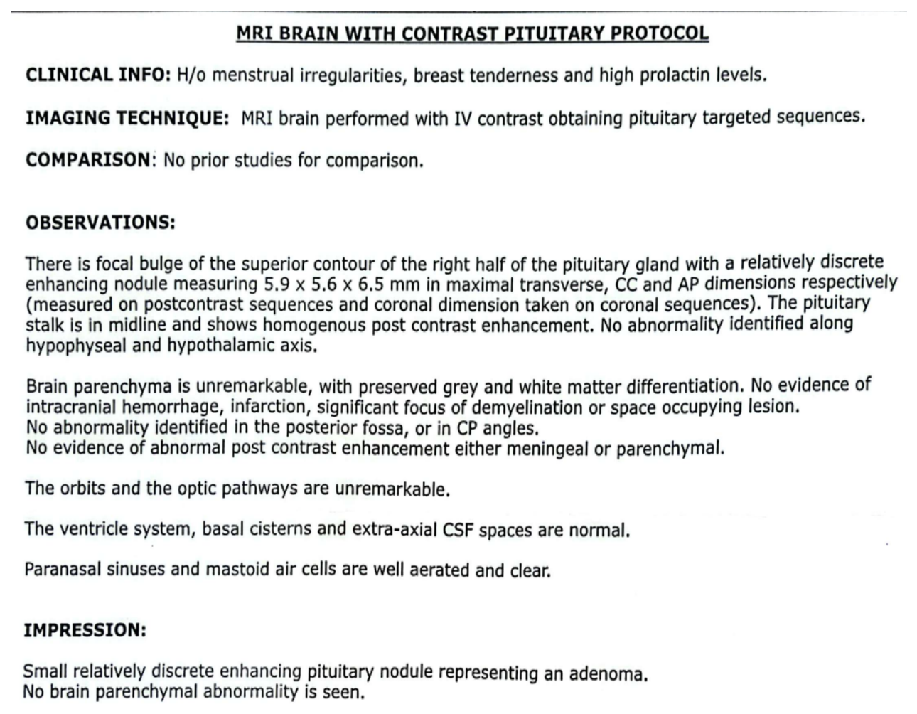
Figure 2 presents the MRI report of a patient diagnosed with a pituitary tumor, highlighting the initial size of the tumor.

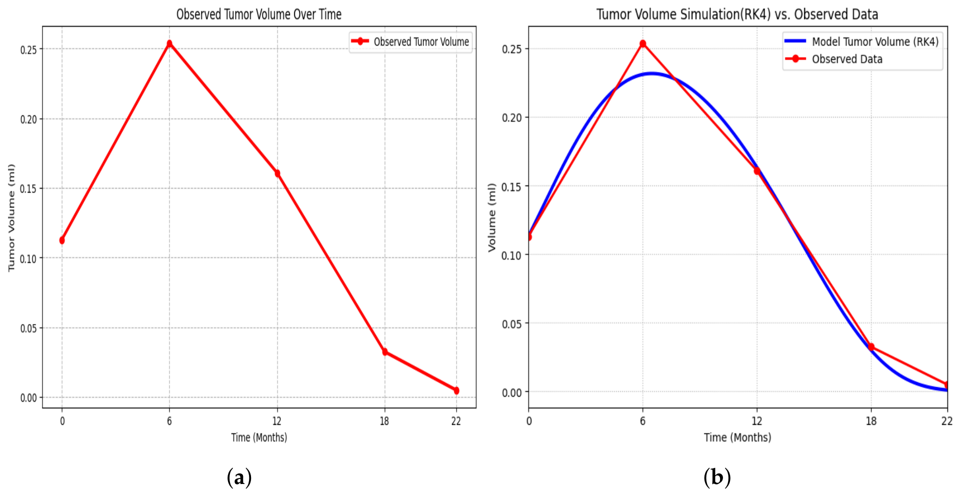
Figure 3a shows the longitudinal clinical measurements of a patient diagnosed with a pituitary tumor, where tumor volumes (in mL) have been recorded at several follow-up meetings, as listed in

Table 2. Tumor volume in (mm) and (mL).

Sr. No.	Tumor Size (mm)	Tumor Volume (mL)
1	$5.9\times 5.6\times 6.5$	$0.113$
2	$9\times 9\times 6$	$0.254$
3	$8\times 7\times 5.5$	$0.161$
4	$4.44\times 4\times 3.5$	$0.0325$
5	$2.9\times 2.55\times 1.3$	$0.0050$

. Following vaccination, the tumor progressed and then began to shrink over time. By approximately twenty-two months, the tumor volume had declined to near zero, indicating the recovery of the patient.

Based on the available information, a mathematical model was formulated and numerically solved using the fourth-order Runge–Kutta method. The resulting numerical solution was then compared with the clinical data, as illustrated in Figure 3b.

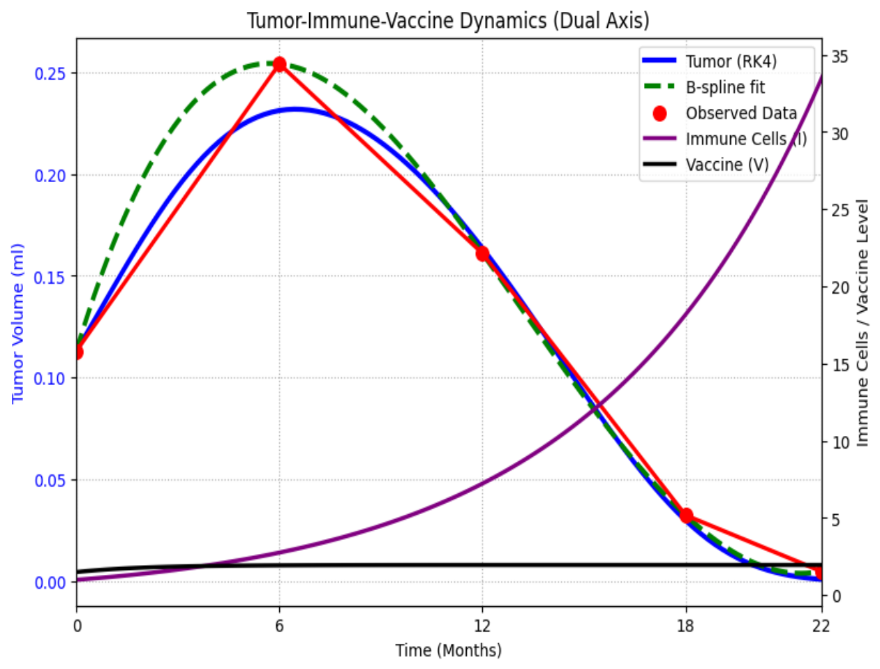
Figure 4 demonstrates the behavior of tumor and immune cells along with the vaccine. From the figure, it can be seen that the observed data and numerical outcomes show identical behavior with minimum error, i.e., at first the tumor increases, then with the passage of time and the administration of constant medication, the tumor decreases. While immune strength is improving with the vaccine. The comparison demonstrates a close agreement between the two datasets, with only minor discrepancies observed in the numerical approximations, as reported in

Table 3. Error comparison.

Time (Months)	Observed	RK4 Value	Absolute Error	RMSE of RK4
0	0.11300	0.11300	0.00000	0.010509
6	0.25400	0.23112	0.02288
12	0.16100	0.16357	0.00257
18	0.03250	0.02995	0.00255
22	0.00500	0.00104	0.00396

.

Physically, this comparison indicates that key processes like tumor, immune, and vaccine interaction are expressed correctly, and small variation or error in approximate results shows the variability in parameters or modeling uncertainties, and the model’s ability to describe tumor progression or suppression is validated by this comparison.

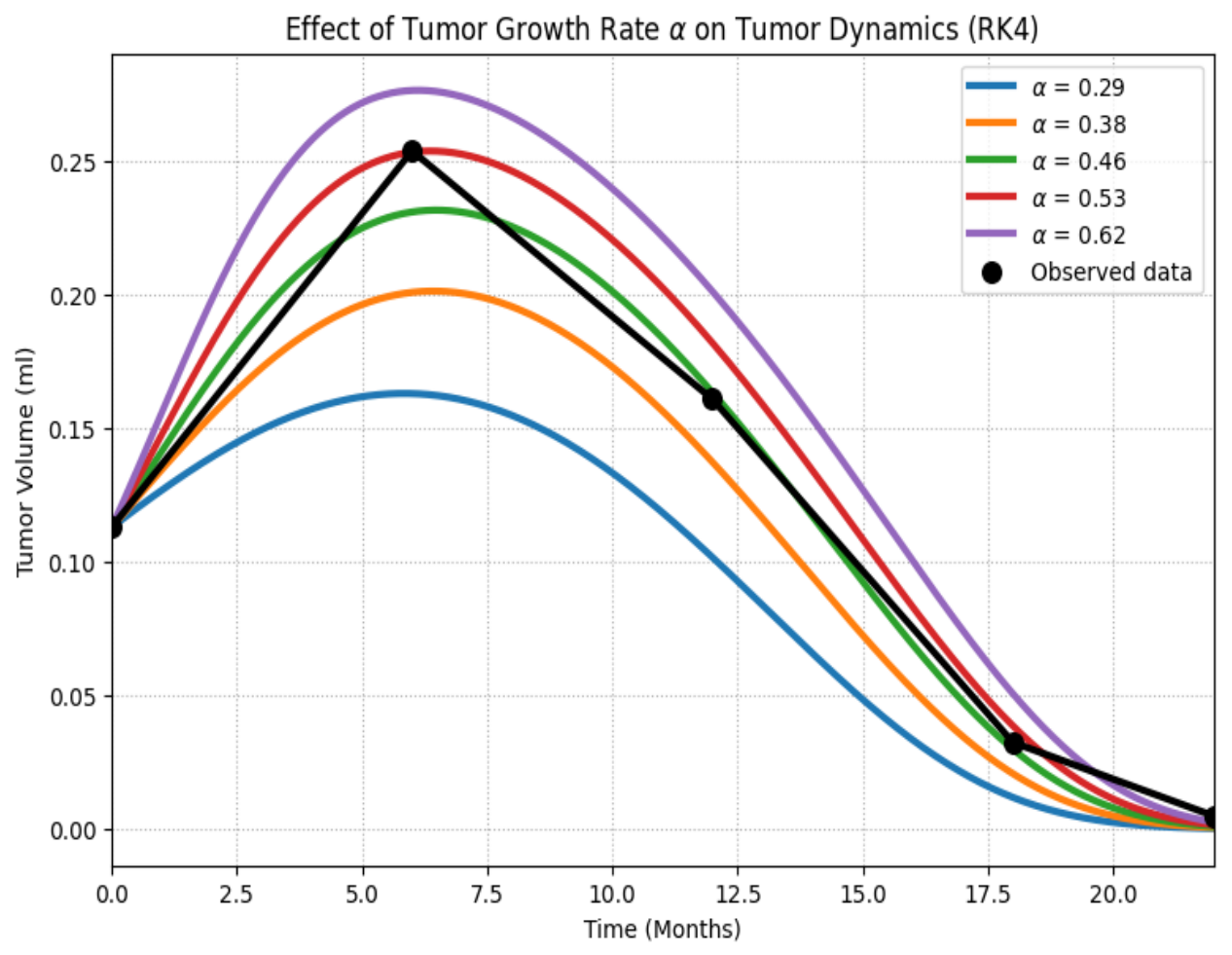
The influence of the tumor growth rate $\alpha$ is illustrated in Figure 5. The results show that for larger values of the growth rate (e.g., $\alpha =0.62$), tumor progression is more pronounced, indicating slower tumor elimination and the need for adjustment of other model parameters. In contrast, smaller values of $\alpha$ lead to reduced tumor growth and faster eradication. The case $\alpha =0.46$ provides the best agreement between the numerical simulations and the clinical data. 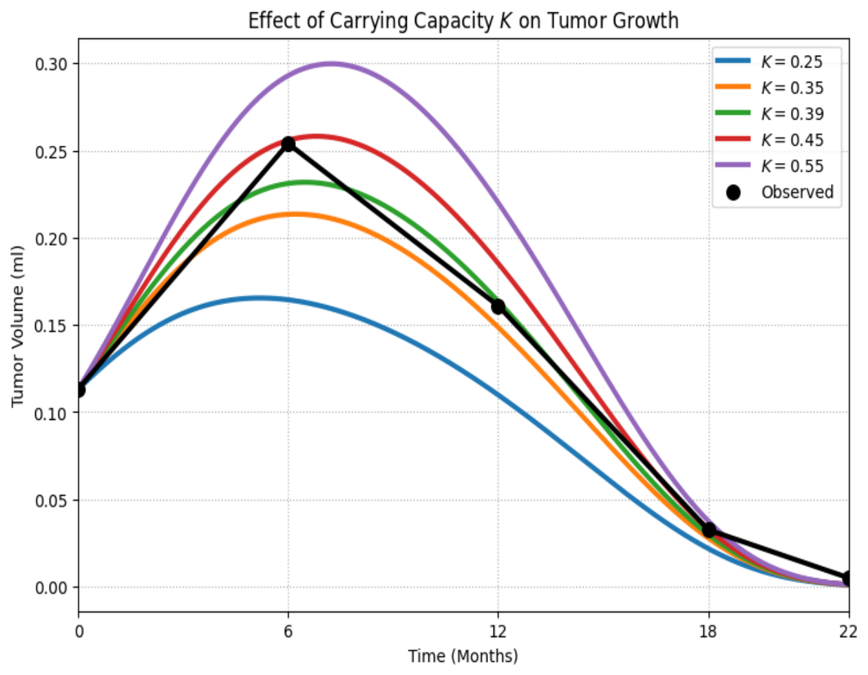Figure 6 illustrates the effect of the carrying capacity on tumor dynamics. From a biological perspective, larger values of K (for example, $K=0.55$) permit more rapid and sustained tumor growth, whereas smaller values of K (such as $K=0.25$) lead to slower tumor expansion, as observed in Figure 6.

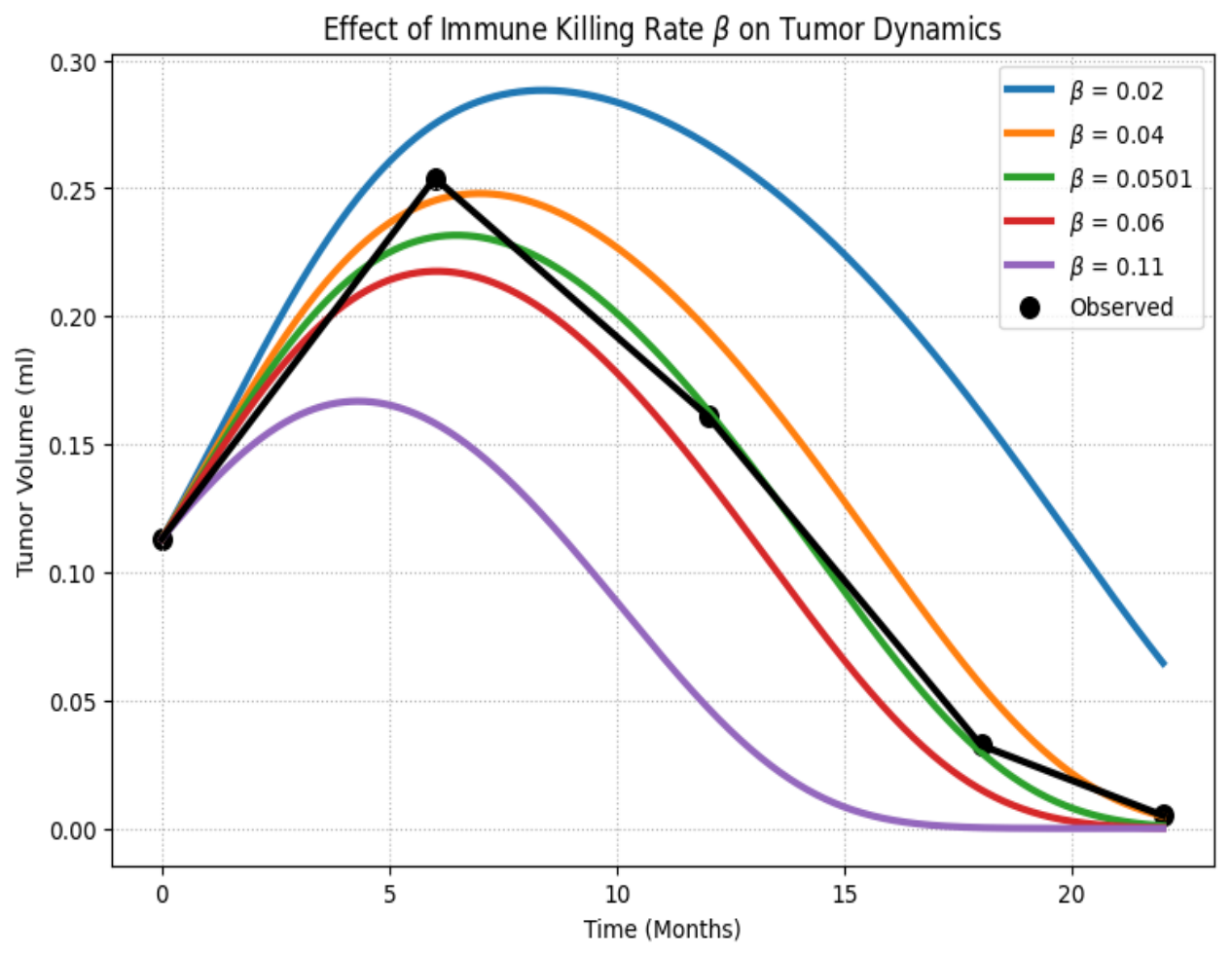
Figure 7 illustrates the influence of $\beta$ on tumors, and it can be noticed that as $\beta$ takes larger values (i.e., $\beta =0.11$) the tumor growth suppresses rapidly, indicating a strong immune response, and for smaller values like $\beta =0.02$, tumor elimination slows down, resulting in a weaker immune response.

Biologically, the immune killing rate is defined as the capacity of immune cells to eliminate tumor cells. Clinically, larger values of the immune killing rate means strong immune response and faster tumor eradication, whereas smaller values of the immune killing rate means a weak immune response, resulting in slower tumor destruction.

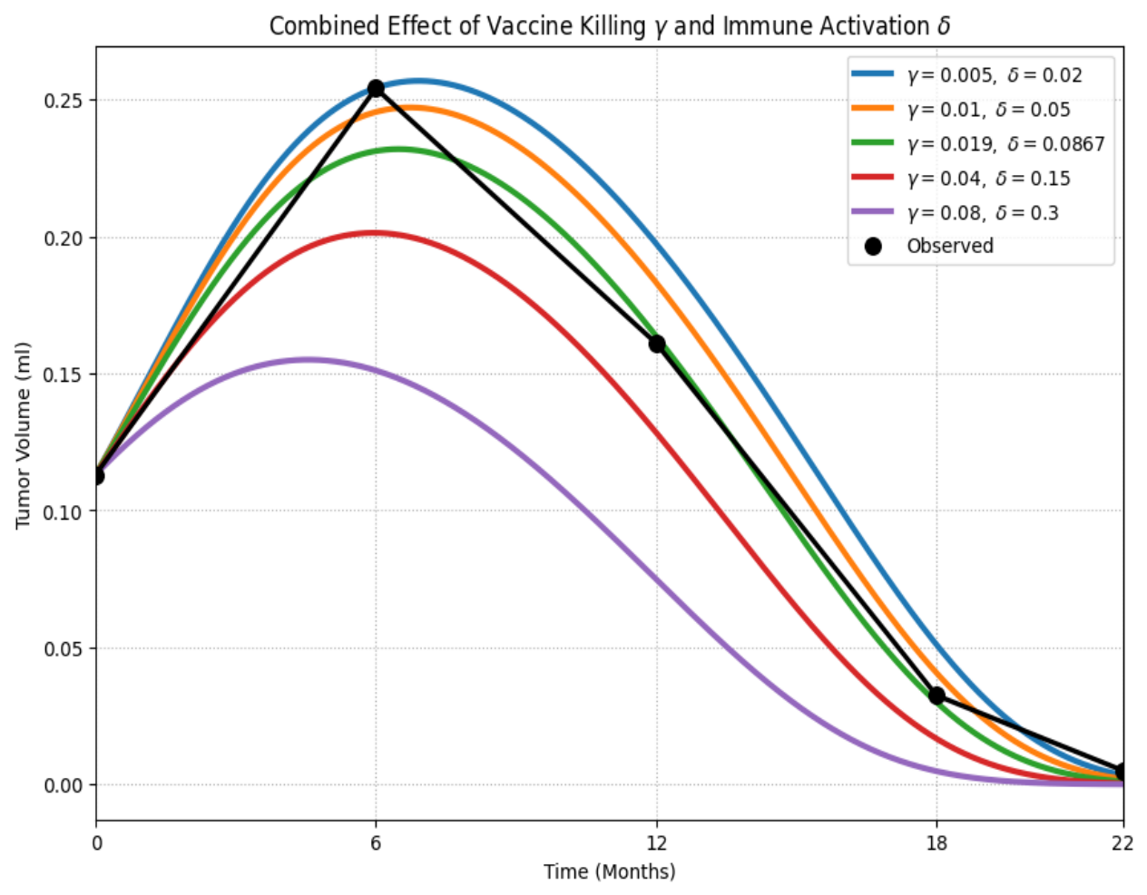
Figure 8 expresses the combined effect of the vaccine killing tumor $\gamma$ and immune activation rate $\delta$ on tumor. Biologically, both parameters play an important role in destroying tumor cells. Higher values of both parameters indicate faster destruction of tumor cells, while smaller values of $\gamma$ and $\delta$ show a slower decline in tumor volume. From Figure 8, it can be seen that, for γ = 0.08, and δ = 0.3, vaccine and immune cells simultaneously eradicate the tumor rapidly (see purple line in graph), indicating the effectiveness of the vaccine. On the other hand, if either parameter takes a smaller value, indicating slower or incomplete reduction in the tumor, this indicates the poor effectiveness of the vaccine and the immune system.

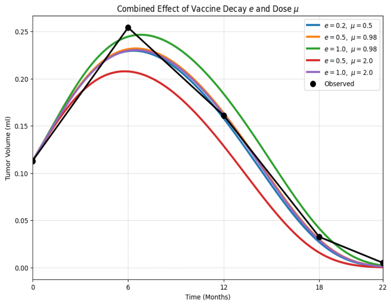
The graphical behavior of the impact of vaccine influx and decay rate on the tumor is expressed in Figure 9. It can be observed that for smaller values of drug decay and higher influx rate of vaccine (i.e., $e=0.5$ and $\mu =2.0$), the tumor declines more rapidly as compared to a smaller influx rate and a higher vaccine decay rate.

6. Conclusions

Pituitary adenoma progression is governed by complex interactions among tumor cells, immune responses, and therapeutic interventions. To investigate these dynamics, a tumor–immune–vaccine model based on ordinary differential equations was developed and analyzed. Fundamental properties of the system, including positivity, existence, uniqueness, and stability of equilibrium states, were established analytically. Numerical simulations obtained through the classical RK4 scheme and low RMSE values demonstrated good agreement between model predictions and clinical observations, indicating that the proposed tumor–immune–vaccine model successfully captured the observed tumor regression and may serve as a useful tool for evaluating treatment response. Parameter analysis showed that tumor growth parameters increase tumor burden, whereas immune- and vaccine-mediated mechanisms suppress tumor progression. Notably, enhanced immune killing and vaccine efficacy significantly reduced tumor volume, highlighting the importance of immune activation in controlling pituitary adenoma growth. The present model is restricted to tumor cells, immune cells, and vaccine dynamics, and does not account for additional biological mechanisms such as cytotoxic T cells, dendritic cells, angiogenesis, tumor-induced immune stimulation, immune suppression/exhaustion, or other therapeutic modalities. From a mathematical perspective, advanced analyses including bifurcation analysis, global sensitivity analysis, data-driven approaches, and optimal control investigations will be explored in future work to provide deeper insight into tumor–immune–vaccine dynamics together with other multicellular components.

This work can be used as a foundation for new researchers to develop even more complex patient-specific models aligned with treatment mechanisms.