


Abstract
Accurate aerodynamic modeling of aircraft during post-stall maneuvers remains challenging due to massive flow separation, vortex breakdown, and unsteady hysteresis. This paper presents a gray-box system identification framework that integrates a Long Short-Term Memory (LSTM) network into the physical equations of aircraft motion. Unlike black-box methods that sacrifice interpretability, the proposed architecture preserves the rigid-body Newton-Euler equations while replacing empirical aerodynamic coefficient models with an LSTM network. The LSTM directly predicts the aerodynamic coefficients, which are transformed into forces and moments via exact physical laws, ensuring hard constraint satisfaction. Validation using real flight test data from a large-scale (3/8) fighter aircraft at angles of attack up to 80° demonstrates that the method achieves regression coefficients exceeding 0.96 for all coefficients on unseen data, with near-zero mean errors. Quantitative comparisons show that the proposed method reduces prediction error by 50–70% compared to black-box LSTM and PINN baselines. The framework offers a practical balance of accuracy, interpretability, and extrapolation reliability for post-stall aerodynamic identification.
1. Introduction
The pursuit of high agility and supermaneuverability in next-generation fighter aircraft has made the characterization of unsteady aerodynamics at high angles of attack (AoA) a critical focus of aerospace research. During post-stall maneuvers—such as the Herbst maneuver or the Pugachev Cobra—aircraft experience complex flow phenomena including massive separation, asymmetric vortex shedding, and vortex breakdown. These conditions result in aerodynamic loads that exhibit significant nonlinearities and time-dependent hysteresis, where the forces and moments depend on both the instantaneous flight state and the motion history. Consequently, traditional modeling techniques based on steady-state databases and linear interpolation are insufficient for high-fidelity flight simulation and the design of robust control systems. Accurately identifying the dynamic parameters of aircraft under such conditions is fundamental to ensuring flight stability and safety [1], and validating flight control laws for agile platforms [2].
Conventional expert-experience-informed models, which can be categorized as white-box or structural gray-box methods, established the earliest foundations for aircraft dynamic identification. Goman and Khrabrov proposed a state-space modeling approach that introduced internal state variables to represent the airflow separation point [3]. This method provides physical interpretability by mapping macroscopic flow changes to aerodynamic loads. Mi et al. further extended this model by incorporating influencing factors like reduced frequency and oscillation amplitude to better capture dynamic variations [4]. Complementing these are indicial function models which utilize the response to a step change in motion to predict unsteady loads through convolution integrals, a concept further applied by Ghoreyshi and Cummings to model maneuvering control surfaces [5]. Despite their utility, Fan and Lutze observed that these structural models often struggle with complex, multi-degree-of-freedom (multi-DOF) coupled mechanisms [6].
With the growth of computational power, data-driven black-box models have emerged as a versatile alternative. They map inputs directly to outputs, bypassing complex physical derivations. Early efforts utilized Support Vector Machines (SVM) and Least Squares Support Vector Machines (LS-SVM) to model nonlinear forces. Chen et al. demonstrated that LS-SVM, when paired with specific excitation designs, could effectively capture the initial process of entering hysteresis loops [7], while Wang et al. used SVM to predict aerodynamic coefficients under arbitrary high-AoA motions [8]. Alkhedher provided a comparative study of Artificial Neural Networks (ANN) and Adaptive Neuro-Fuzzy Inference Systems (ANFIS), concluding that ANFIS models often exhibit superior accuracy, although they lack physical significance [9]. Yetkin et al. surveyed a wide array of AI methods, noting their promise for fast coefficient calculation while highlighting the “black-box” challenge of limited interpretability [10]. Additionally, Cheng et al. reviewed the applicability of these intelligent models, noting that they significantly outperform conventional models in constructing nonlinear mapping relations [11].
To address temporal dependencies, Recurrent Neural Networks (RNN) and their variants have become standard. Ignatyev and Khrabrov conducted a comparative study proving that RNNs are significantly more effective at modeling time-lag effects at high AoA compared to feed-forward architectures [12]. Building on this, Long Short-Term Memory (LSTM) networks were developed to solve the vanishing gradient problem. Li et al. successfully applied LSTM to model unsteady aerodynamics across multiple Mach numbers, demonstrating its ability to discover hidden patterns in high-dimensional datasets [13]. Kou and Zhang reviewed these data-driven reduced-order models, highlighting LSTM’s capability to handle the memory effects of the flow field [14]. Furthermore, Suresh et al. used RNNs to model lift coefficients from experimental data, incorporating generalization errors to ensure robustness [15], while George and Raol explored RNNs for parameter estimation using Lyapunov stability analysis [16].
Recognizing the trade-offs between accuracy and interpretability, researchers have developed hybrid or gray-box identification methods. A prominent approach is the Physics-Informed Neural Network (PINN) framework, defined by Raissi et al., where physical laws are integrated into the network loss function [17]. Yan et al. enhanced this framework using transfer learning and adaptive activation functions to improve convergence for carrier-based aircraft landing [18]. Similarly, Liu et al. proposed the DEM-LSTM model, which uses an LSTM to learn the parameters of a differential equation model (DEM), effectively combining data-driven flexibility with structural constraints [19]. These gray-box strategies, as discussed by Wang et al. regarding the Multi-fidelity Neural Network (MFNN), aim to provide models that are both accurate and physically consistent even when experimental data is sparse [20].
Further advanced fusion and integrated frameworks have leveraged multi-fidelity data and complex features. The Weighted Feature Fusion Model (WFFM) proposed by Dong et al. combines a state-space model with an LSTM network through a standardization and weighting layer [21]. This architecture establishes dual mappings: one from states to loads and another from low-fidelity trends to high-fidelity corrections. In a similar vein, Ma et al. introduced a Residual Transformer (ResTrans) autoencoder fused with a deep neural network to extract both temporal and spatial features [22]. Furthermore, Xiong et al. utilized point cloud deep neural networks for aerodynamic prediction, representing 3D geometry as a direct input feature [23].
In complex, noisy environments, online and adaptive identification is necessary. Xu et al. developed an online method using LS-SVM combined with the Unscented Kalman Filter (UKF), transforming identification into a state estimation problem [24]. For multi-DOF maneuvers, Dong et al. [25] utilized attention mechanisms to identify specific state variables that most significantly influence each coefficient. Marques and Anderson utilized finite memory neural networks to reflect the history of transonic loads [26], while Verma and Peyada applied extreme learning machines for near-stall parameter estimation [27]. Finally, Wu et al. proposed generative deep learning for airfoil flow field prediction [28], and Hou et al. demonstrated detection of aerodynamic disturbances using surface pressure and LSTM [29]. For additional studies on related topics, the reader is referred to [30,31].
Recent advances in neural network-based aerodynamic modeling have explored both nonlinear control strategies and algebraic frameworks, yet significant gaps remain for post-stall identification [32,33,34]. Bekhiti et al. [33] proposed a nonlinear adaptive control strategy for the Su-30 fighter aircraft integrating NDI, RBF neural networks, and pure-pursuit guidance, validated through Software-in-the-Loop simulations with Microsoft Flight Simulator 2004. In a separate work, Bekhiti et al. [34] developed an algebraic framework for operator matrix polynomials with applications to aeroelasticity, combining spectral factorization and block-pole assignment with a compact neural compensator for a two-degree-of-freedom aeroelastic wing. Compared to their control strategy [33], the present work uses real flight test data rather than simulation, eliminates the need for a pre-existing baseline model, and hard-codes the Newton-Euler equations as physical constraints rather than relying on NDI inversion. Compared to their algebraic framework [34], which focuses on aeroelastic wing flutter suppression with a shallow neural corrector, the proposed method addresses full six-degree-of-freedom aircraft dynamics under post-stall conditions, employs a deep LSTM architecture with gating mechanisms for temporal dependencies, and directly predicts aerodynamic coefficients rather than providing corrective terms. Thus, the proposed LSTM-driven gray-box framework uniquely combines temporal learning with hard-coded physics for post-stall aerodynamic identification, complementing the control-oriented and algebraically focused works of Bekhiti et al.
Despite significant progress in both pure data-driven modeling and hybrid physics-informed strategies, a critical challenge remains: how to best integrate temporal neural architectures into the existing physical frameworks of aircraft dynamics. While traditional black-box models excel at capturing high-dimensional nonlinearities, they often fail to provide the engineering reliability required for aggressive flight regimes. Conversely, conventional gray-box methods rely on pre-defined empirical expressions that cannot adequately capture the complex, time-dependent hysteresis characteristics of post-stall aerodynamics. The novelty of this research is threefold: (1) Direct embedding of LSTM gating into the inverse dynamics: Unlike previous hybrid methods that use neural networks as function approximators external to the physical model, our approach replaces the empirical aerodynamic coefficient functions with an LSTM network that receives the full temporal history of state and control inputs. The network’s forget, input, and output gates operate directly on the aerodynamic coefficient estimation problem, allowing the model to autonomously determine which past states influence current aerodynamic loads—a capability impossible with fixed-structure gray-box models. (2) Preservation of physical structure with data-driven flexibility: The proposed architecture maintains the rigid-body equations of motion exactly as derived from Newton-Euler principles. Only the aerodynamic coefficient terms —which are fundamentally uncertain in post-stall regimes—are learned from data. This selective learning ensures that all predictions remain physically consistent with conservation laws while gaining the flexibility to represent arbitrary nonlinearities. (3) Intrinsic temporal coupling versus superficial constraint layering: Previous physics-informed neural network (PINN) approaches incorporate physical laws only through additional loss function terms, creating a soft constraint that can be violated during inference. In contrast, our LSTM-driven gray-box architecture hard-codes the physical structure into the network’s forward pass: the LSTM outputs aerodynamic coefficients, which are then transformed back to forces and moments and fed into the rigid-body dynamics. The network cannot produce a prediction that violates Newton’s laws because the physical model is embedded in the prediction pipeline itself, not merely in the loss function.
The proposed LSTM-driven gray-box architecture achieves superior physical interpretability through three fundamental mechanisms that distinguish it from alternative modeling approaches. First, unlike purely black-box methods that learn direct mappings from states to forces or moments—treating the aircraft as an input-output system with no internal structure—our approach constrains the LSTM to predict only the six aerodynamic coefficients, quantities that possess direct physical meaning in flight mechanics. Engineers can therefore inspect these coefficient predictions to diagnose model behavior, verify compliance with physical expectations (e.g., lift coefficient increasing with angle of attack up to stall), and relate identified patterns to actual aerodynamic phenomena such as vortex breakdown or flow separation. Second, in contrast to Physics-Informed Neural Networks (PINNs) that incorporate physical laws only as soft penalty terms in the loss function—allowing the network to produce physically impossible predictions when extrapolating beyond training data—our approach hard-codes the Newton-Euler equations directly into the network’s forward pass. The rigid-body dynamics are executed using exact analytical expressions; the LSTM cannot bypass or violate these equations regardless of input conditions. This guarantees that all predictions respect conservation of translational and angular momentum, a critical requirement for engineering applications such as flight control law validation. Third, unlike conventional gray-box models that rely on pre-defined empirical expressions with fixed mathematical structures (e.g., first-order lags or convolution kernels) to represent unsteady effects, our LSTM-based approach learns the temporal dependence structure directly from data. The network’s gate activations—forget, input, and output gates—can be analyzed post-training to reveal which past time steps most strongly influence current aerodynamic predictions, providing insight into the effective memory horizon of the unsteady flow phenomena. For example, high forget gate values indicate that past states are being retained, suggesting long-term hysteresis effects, while rapid decay of cell state information suggests dominance of recent history. This level of diagnostic insight is impossible to obtain from black-box networks or fixed-structure empirical models, establishing the proposed method as a genuinely interpretable gray-box approach that balances the flexibility of deep learning with the transparency of physics-based modeling.
2. Gray-Box Approach for Aircraft System Identification
2.1. Aircraft Model
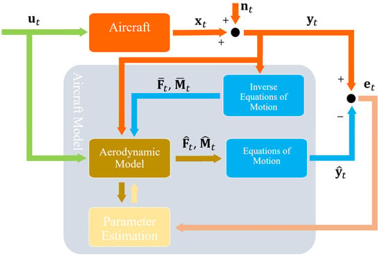
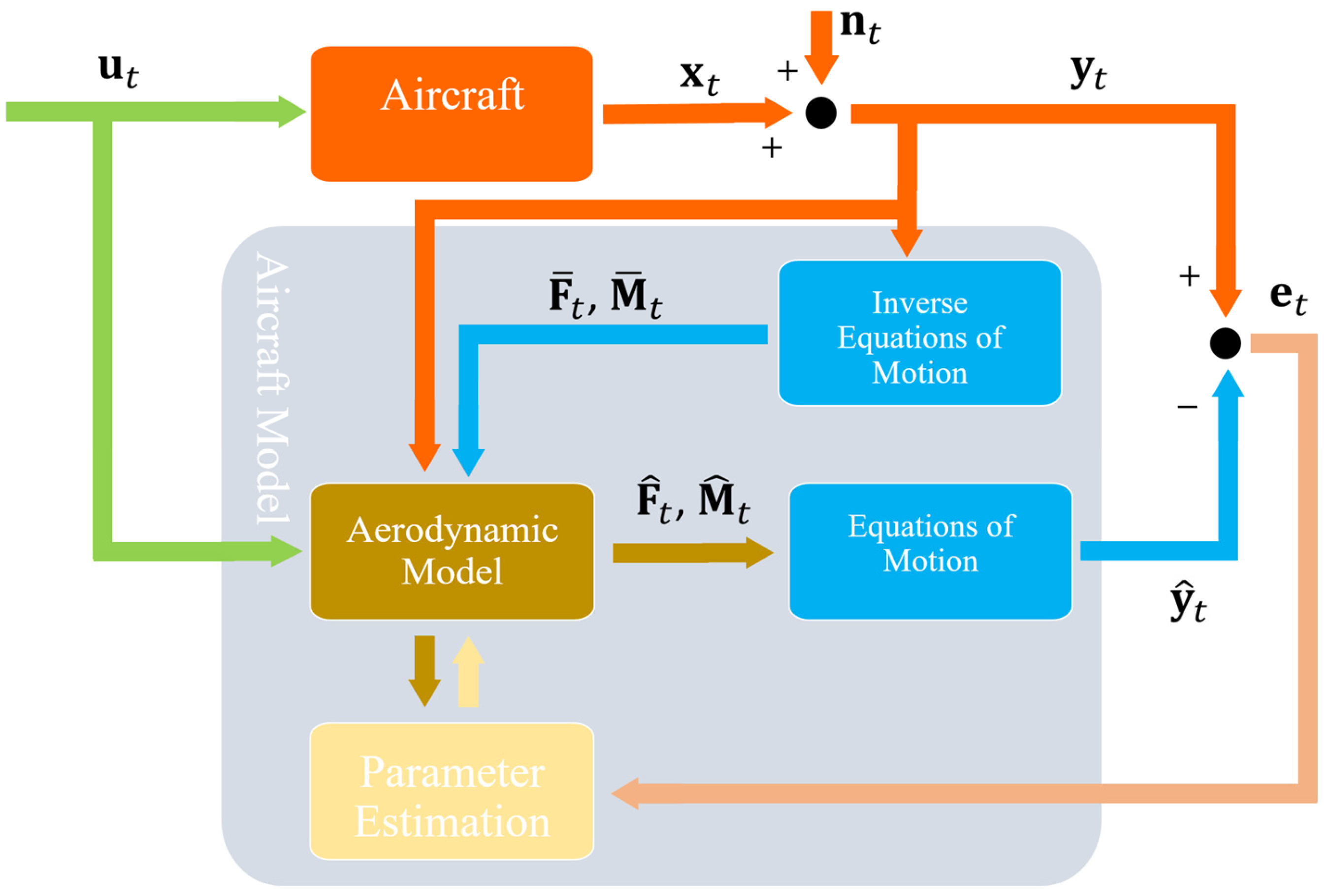
Gray-box identification represents a hybrid approach that combines the physical insight from first-principles modeling with the flexibility of data-driven techniques. In aircraft applications, this method retains the fundamental structure of the rigid-body equations of motion derived from Newton-Euler formalism—including the kinematic and kinetic relationships governing translational and rotational degrees of freedom—while using flight data to estimate uncertain aerodynamic force and moments that cannot be reliably obtained from analytical methods or wind tunnel tests. Therefore, the aerodynamic forces and moments are calculated by reverse equations of motion, and inputted to the model as the responses. For post-stall maneuvers, gray-box approaches are particularly valuable because the Newtonian mechanics describing aircraft motion remain valid even in extreme flight conditions, but the aerodynamic models embedded within these equations become highly uncertain due to separated flows and unsteady effects. This approach reduces the parameter space that must be identified—focusing only on the aerodynamic coefficients rather than the entire system dynamics—which typically necessitates less training data and yields more robust models with clearer physical meaning, enabling engineers to relate identified parameters to actual aerodynamic phenomena. In Figure 1, the gray-box method of aircraft system identification is shown.
Figure 1.
The gray-box method of aircraft system identification. [arrows: signals, boxes: systems/models, dots: add/subtract actions].
2.2. Assumptions
To isolate and rigorously study the aerodynamics of post-stall flight, the aircraft in this investigation is subjected to a set of simplifying yet physically plausible assumptions, including rigid body symmetry, unpowered flight, constant mass and inertia, static atmosphere, and flat-Earth approximation. Under these conditions, the rigid-body dynamics are fully described by the Newton-Euler equations, but the core challenge—and the focus of this work—lies in accurately identifying the aerodynamic force and moments that govern the right-hand side of these equations, particularly the nonlinear and unsteady coefficients that dominate in the post-stall regime.
2.3. Equations of Motion
The dynamic behavior of an aircraft is governed by a system of first-order, nonlinear, and strongly coupled differential equations. These equations serve as the mathematical foundation for flight dynamics analysis, taking aerodynamic forces and moments as inputs and producing the time evolution of flight variables, including linear and angular velocities, Euler angles, and position coordinates. In post-stall maneuvering, where conventional linearized models become invalid due to large angular excursions and highly nonlinear aerodynamics, the full nonlinear form of these equations must be retained.
According to Newton’s second law applied in the body-fixed reference frame, the translational dynamics are expressed as:
Similarly, Euler’s equations governing rotational motion are given by:
The kinematic relationships, derived from Euler angle propagation, relate angular velocities to the rate of change of aircraft attitude:
While body-velocity components, i.e., , provide a complete description of translational state, it is advantageous to reparametrize in terms of total velocity , angle of attack , and sideslip angle in the given dynamic pressure . This transformation, given below, is motivated by two considerations: these quantities can be measured directly from flight data, and aerodynamic forces exhibit more meaningful relationships with them:
Also, one can find the altitude based on the Navigation Equation, as follows:
2.4. Inverse Equations of Motion
In the equation error approach, which forms the foundation of many aircraft system identification methods, the aerodynamic force and moment coefficients are treated as dependent variables to be estimated from measured flight data. These coefficients are subsequently expressed as functions of independent regressors through a suitable model structure. The model parameters are then selected to minimize the sum of squared errors between the predicted coefficients and those derived from measurements across all six degrees of freedom. This method is particularly well-suited for post-stall aerodynamic identification, as it allows for flexible model structures capable of capturing the nonlinear and unsteady phenomena characteristic of high-angle-of-attack flight.
Since aerodynamic forces and moments cannot be measured directly during flight, they must be reconstructed from other measured quantities using the inverse form of the aircraft equations of motion. The required equations are derived by rearranging the translational and rotational dynamics from the previous subsection, solving explicitly for the aerodynamic force and moment coefficients. This inverse formulation effectively treats the aircraft as an “aerodynamic balance” in flight, where the observed motion provides insight into the underlying aerodynamic mechanisms.
The force and moment equations in the body-fixed reference frame are rearranged to isolate the aerodynamic force and moment components:
In the above equations, several quantities are obtained directly from measurements: the Euler angles are obtained by vertical gyros, the angular velocities are acquired by rate gyros, the translational accelerations are achieved by 3-axis accelerometers, and the airspeed , angle of attack , and sideslip angle are acquired by air data probes. The aircraft mass and inertia tensor are determined from ground-based measurements, including weight and balance procedures, prior to flight. Angular accelerations cannot be measured directly. They are obtained through smoothed numerical differentiation of the measured angular velocity time histories.
3. The LSTM Network
3.1. Memory Cells
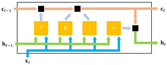
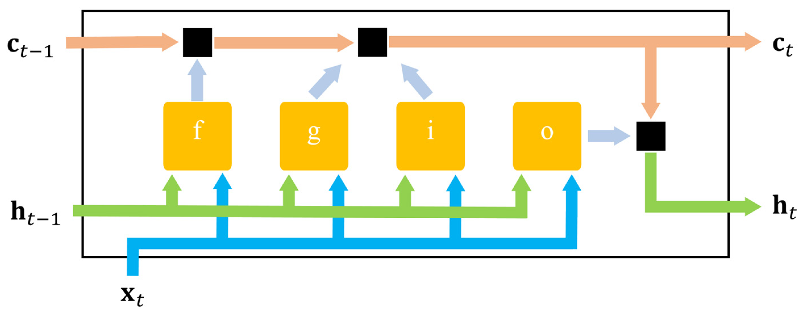
The LSTM memory cell regulates information flow through a gating architecture comprising three gates. The forget gate determines what previous information to discard. The input gate and candidate cell work together to store new information. The output gate controls what information propagates to subsequent time steps. This coordinated mechanism enables the memory cell to preserve critical information across long sequences while discarding obsolete content, effectively addressing the vanishing gradient problem and allowing the network to learn complex temporal dependencies.
The flowchart of a memory cells and its gates are illustrated in Figure 2. In this figure, and are the hidden and cell state vectors, respectively, while is the input vector. The , , , and are the forget gate, cell candidate, input gate, and output gate, respectively. At each time step , the LSTM cell receives the previous hidden state and the previous cell state and through the coordinated operation of its gates, it selectively forgets parts of , adds new information from the current input and the cell candidate to create new cell states , and then filters this updated cell state to produce the new hidden state .
Figure 2.
LSTM memory cell flow: input flows through forget, input, and output gates to produce the hidden state. [yellow blocks: gates, black squares: operations of forget, update, and output of the gates, blue arrows: inputs, green arrows: hidden states, copper arrows: cell states].
3.2. The Learnable Parameters
The learnable parameters within an LSTM layer are organized into three primary matrices: the input weights , the recurrent weights , and the bias vector . These matrices are not monolithic but are formed by vertically stacking the corresponding parameters for each of the four internal gates. This structuring is represented mathematically as:
In this notation, the subscripts , , , and correspond to the input gate, forget gate, cell candidate, and output gate, respectively.
The evolution of the layer’s memory is governed by two key state vectors:
- The cell state, which serves as the long-term memory, is updated at each time step according to:
Here, represents element-wise multiplication.
- The hidden state, which represents the short-term or output state, is then derived from the updated cell state:
The function is the state activation function.
The computation of the four internal components that control this memory update is detailed in the following set of equations. At each time step , the gates and the candidate cell are calculated using the current input and the previous hidden state :
As can be seen, the input weights are applied directly to the current input data , projecting it into the network’s internal space. Concurrently, the recurrent weights are applied to the previous hidden states , allowing the network to incorporate its own past activations. Finally, the bias is added. This combined, weighted sum is then passed through the specific activation functions (typically sigmoid for gates and tanh for the cell candidate) that govern the behavior of the input, forget, and output gates, as well as the cell state update.
3.3. The LSTM Layer
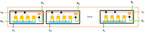
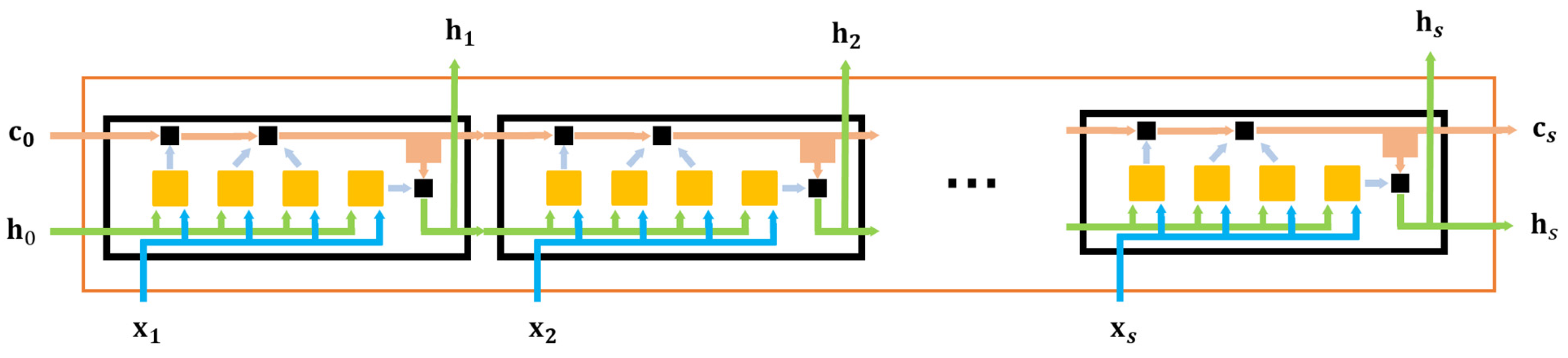
The LSTM layer is a recurrent neural network architecture distinguished by its array of memory cells, each functioning as a self-contained unit capable of maintaining and regulating information across extended temporal sequences. These memory cells collectively enable the layer to overcome the limitations of traditional recurrent networks by providing a mechanism for preserving long-term dependencies without experiencing the vanishing gradient problem. At each time step, every memory cell receives the current input and the previous hidden state, and through its internal gating architecture, produces an updated hidden state and cell state. The cell state serves as a long-term memory conduit that runs across time steps, while the hidden state represents the layer’s output at each step and carries information forward to subsequent time steps. When configured for sequence-to-sequence regression, the LSTM layer outputs the hidden state at every time step, producing a sequence of the same length as the input or, within an encoder–decoder framework, generating a new sequence of potentially different length. Multiple LSTM layers can be stacked hierarchically, where the first layer processes the raw input sequence and passes its entire output sequence to the second layer. This stacking enables the network to learn temporal features at different scales, with lower layers capturing short-term dynamics and higher layers extracting more abstract patterns. Figure 3 illustrates the LSTM layer architecture in which time steps are processed.
Figure 3.
LSTM layer processing over time steps: Each cell outputs hidden state to the next step. [yellow blocks: gates, black squares: operations of forget, update, and output of the gates, blue arrows: inputs, green arrows: hidden states, copper arrows: cell states].
3.4. LSTM Network for Sequence-to-Sequence Regression
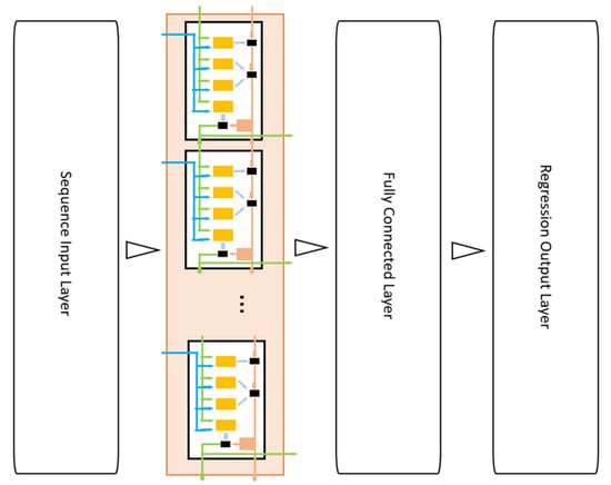
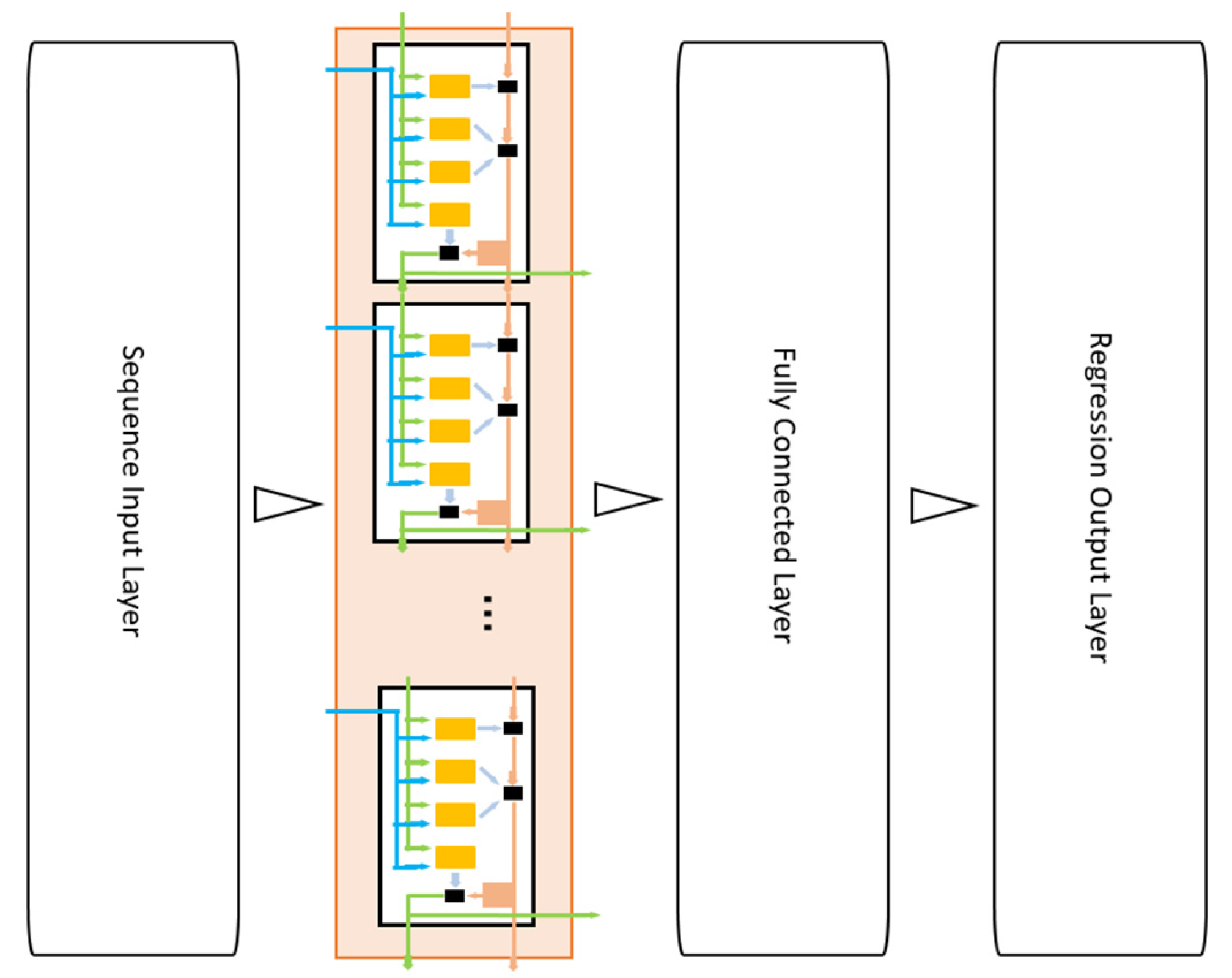
An LSTM network designed for sequence-to-sequence regression is architected to transform an input sequence of continuous values into an output sequence of continuous values, where the two sequences may differ in length. This is achieved by stacking four essential components: a sequence input layer, one or more LSTM layers, a fully connected layer, and a regression output layer. The architecture of the LSTM network designed for sequence-to-sequence regression is illustrated in Figure 4.
Figure 4.
The architecture of the LSTM network designed for sequence-to-sequence regression.
An LSTM network for sequence-to-sequence regression stacks four components: a sequence input layer, one or more LSTM layers, a fully connected layer, and a regression output layer. The input layer preserves temporal ordering and passes formatted data to subsequent layers. The LSTM layers learn temporal dependencies by outputting a hidden state at every time step. When multiple LSTM layers are stacked, each processes the entire hidden state sequence from the previous layer, enabling hierarchical learning of temporal features.
The first layer captures short-term dynamics directly from raw input, while subsequent layers extract more abstract patterns and longer-range dependencies, which is particularly valuable when output depends on patterns spanning multiple timescales.
The fully connected layer maps the high-dimensional LSTM outputs to the desired regression format at each time step. After the final LSTM layer produces a hidden state vector for every step in the output sequence, the fully connected layer applies a linear transformation independently to each vector. This transformation reduces dimensionality from the LSTM hidden size to the output feature size, typically one for univariate regression or the number of target variables for multivariate regression. Because the same learned weights are applied across all time steps, the mapping remains consistent throughout the sequence.
The regression output layer completes the architecture by computing the error between predicted and target sequences during training. It receives transformed values from the fully connected layer and compares them to ground truth using the mean squared error loss, which averages squared differences across all time steps and sequences. This loss drives backpropagation for weight updates. During inference, the layer simply outputs the predicted continuous values, producing the final forecasted sequence such as future stock prices or sensor measurements.
3.5. The Training Process
During training, these weight matrices ( and ) and the bias vector () are iteratively adjusted through backpropagation, enabling the network to learn the optimal transformations for sequence processing. Training optimizes the network by minimizing the Mean Squared Error (MSE) between predicted and target sequences. Forward propagation generates predictions, which are compared to targets via the loss function. Back-Propagation Through Time (BPTT) then computes gradients of the loss with respect to the network parameters. The Adam optimizer uses these gradients to iteratively update the weights. This cycle repeats over the training dataset for many epochs until convergence.
3.6. The Mathematical Formulation of the Gray-Box Coupling
To clarify the mathematical relationship between the physical rigid-body dynamics and the LSTM network, the complete formulation of the proposed gray-box identification framework is presented in this subsection. Unlike black-box methods that learn the entire dynamics, the new approach preserves the known physical structure while using the LSTM exclusively for the uncertain aerodynamic coefficients.
The LSTM network directly predicts the six dimensionless aerodynamic coefficients at each time step
The predicted coefficients are then transformed into aerodynamic forces and moments using the physical definitions:
The loss function for a sequence of length with aerodynamic coefficients is:
where is the calculated aerodynamic coefficient derived from flight data via the inverse equations of motion (6) and (7), and is the LSTM prediction. The predicted forces and moments are then substituted into the rigid-body Equations (1)–(5) to compute the flight parameters and advance the simulation. The distinguishing feature of a gray-box model is the preservation of known physical structure. In our framework:
- Known physics is hard-coded: Equations (1)–(5) are exact analytical expressions derived from Newton-Euler laws. These are never learned or approximated by the neural network.
- Only uncertain components are learned: The LSTM learns only the six aerodynamic quantities that are fundamentally uncertain in post-stall regimes due to flow separation and hysteresis.
- Physical consistency is architectural: Because the LSTM outputs coefficients that are immediately transformed into forces and moments via known physical laws, the network cannot produce predictions that violate momentum conservation. This is a hard constraint, not a soft penalty.
Unlike Physics-Informed Neural Networks (PINNs) that incorporate physical laws as soft penalty terms in the loss function, the proposed approach uses a standard mean squared error (MSE) loss on the aerodynamic coefficients only. No physics-based loss terms are required because physical constraints are hard-coded into the architecture itself. In PINNs, physics losses are added to enforce compliance with governing equations because the network learns the entire solution field. In the proposed approach, the governing Equations (1)–(5) are executed directly using the forces and moments derived from the LSTM’s coefficient predictions. The network cannot bypass or violate these equations. Therefore, any prediction that satisfies the training data implicitly respects the physical laws encoded in the dynamics.
The complete training and inference procedures are summarized in Algorithms 1 and 2.
| Algorithm 1: LSTM-driven gray-box identification framework: the training procedures |
|
| Algorithm 2: LSTM-driven gray-box identification framework: the inference procedures |
|
4. Flight Test Data
The primary objective of this paper is to develop a global aerodynamic model capable of accurately estimating aircraft state variables during complex nonlinear maneuvers, particularly at post-stall maneuvers. To this end, flight test data from a remotely piloted, large-scale (3/8) fighter airplane model, originally tested at the NASA Flight Research Center, are utilized in this study [35]. This unpowered model was a 3/8-scale representation of an advanced air superiority fighter with 45° swept leading-edge wings, twin vertical tails, and a fuselage length of 19.05 m at full scale. The model was constructed primarily of fiberglass with metal load-carrying members and was designed to be as stiff as the full-scale airplane, withstanding loads up to 5 g flight conditions.
The flight tests covered an altitude range from approximately 15,250 m down to 4600 m, with angles of attack reaching up to 80° during erect spins and −70° during inverted spins. Various maneuvers were performed to excite all relevant flight modes, predominantly operating in the nonlinear regime with angles of attack extending well beyond the stall region. The model was equipped with comprehensive instrumentation to acquire flight data at a sampling rate of 200 samples per second. The recorded quantities included Euler angles (pitch, roll, and heading angles measured by a four-gimbal, two-gyro platform system), angular rates (pitching, rolling, and yawing), linear accelerations at the center of gravity (longitudinal, lateral, and normal), airspeed, altitude, and control surface positions (each aileron, rudder, and horizontal stabilizer position). Additionally, angle of attack and sideslip angle were measured using vanes mounted on a boom 5.4 m ahead of the center of gravity, with appropriate corrections applied for local flow deflection, angular rates, and linear accelerations during post-flight data processing. The resolution of the full-scale measurement range ensured that each quantity could be resolved to less than 1 percent of the full-scale recording range, with eight critical quantities (attitudes, rates, and accelerations) recorded with both full and expanded scales in the primary regions of interest.
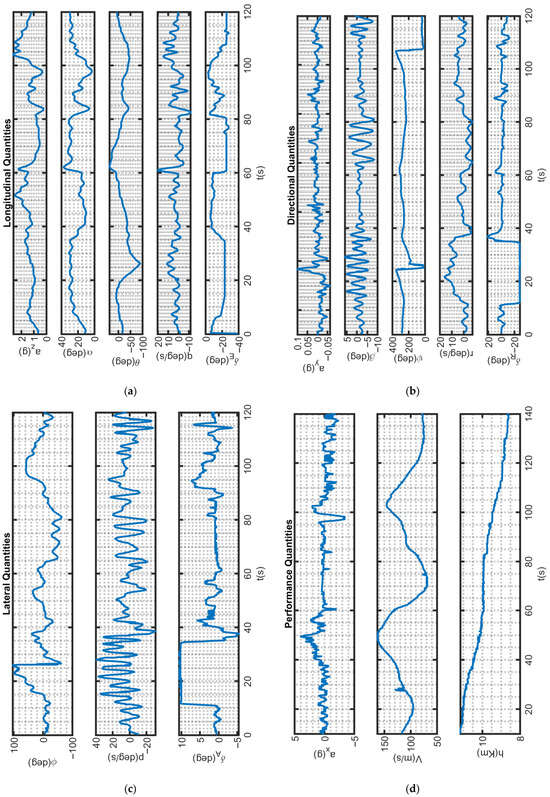
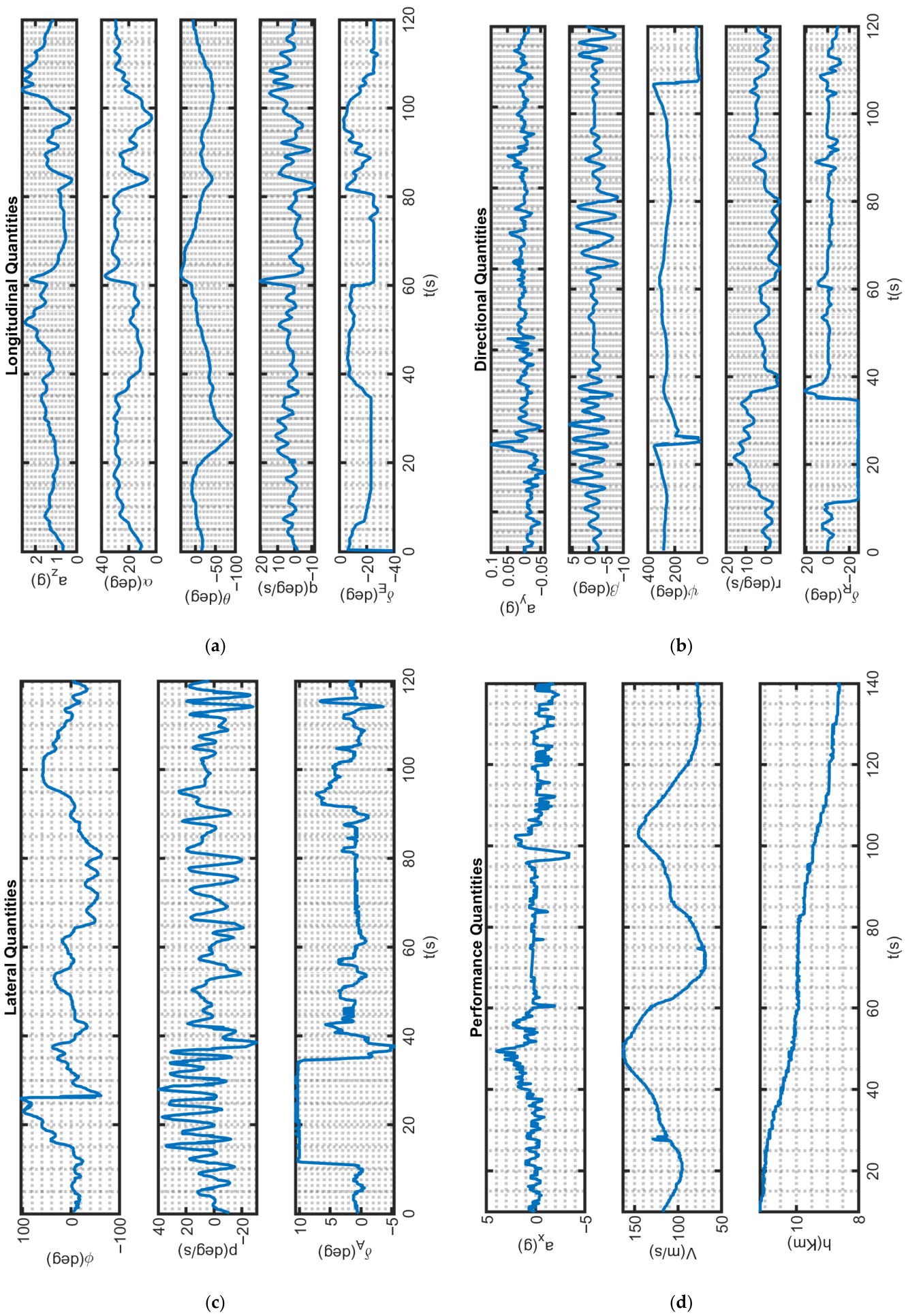
Two distinct sets of flight test data from this aircraft are employed in the present study. The first dataset is used for training the aerodynamic model, while the second dataset is reserved only for model test. The first dataset in shown in Figure 5.
Figure 5.
The training dataset: (a) Longitudinal quantities, (b) Directional quantities, (c) Lateral quantities, (d) Performance quantities.
5. The Utilized Model
5.1. The Regressors and Regressands
The state vector for the aircraft is defined as:
The heading angle and horizontal position coordinates (i.e., latitude and longitude) do not influence aerodynamic forces and moments; therefore, they may be omitted when the objective is purely aerodynamic identification.
The control input vector, commanding aerodynamic surfaces, is defined as:
Both the state vector and the control input vector are the inputs of the aerodynamic model. Therefore, the network has 18 regressors (inputs) for the identification process, namely the summation of 15 flight parameters of the state vector and 3 control command of the control input vector.
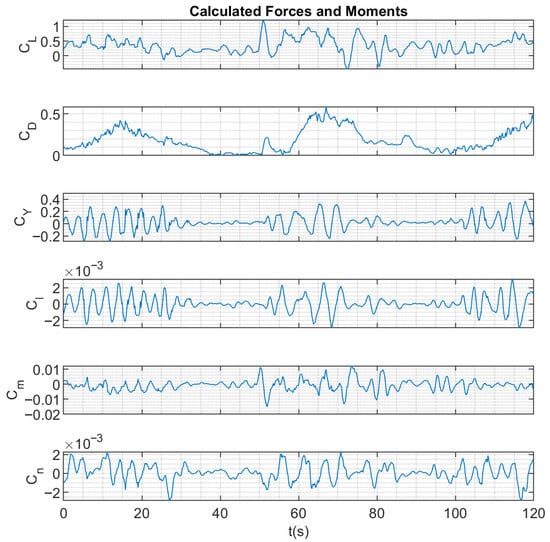
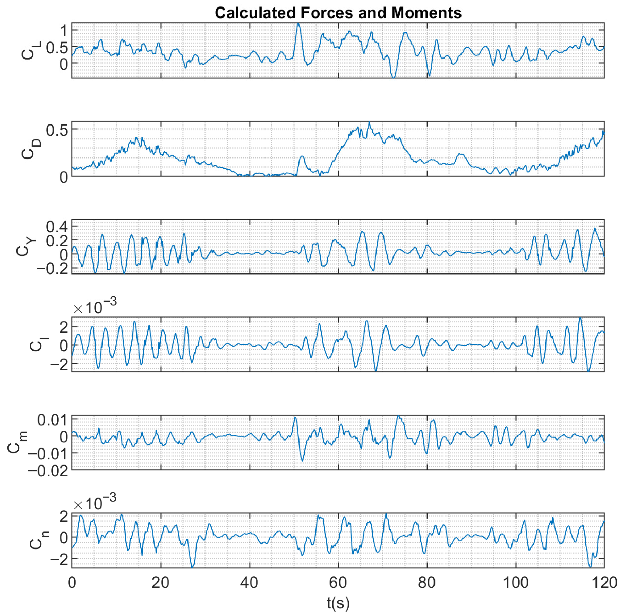
The regressands (targets) of the identification process are the force and moment coefficients. Therefore, there are 6 regressands, namely the lift, drag, sideforce, rolling moment, pitching moment, and yawing moment coefficients. These parameters are obtained from the state vector by the inverse equations of motion, as previously mentioned in sub-Section 2.4. For the training dataset, the regressands are illustrated in Figure 6.
Figure 6.
The regressands for the training dataset.
5.2. The Network Architecture, Learning Algorithm and Parameters
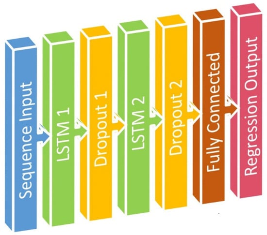
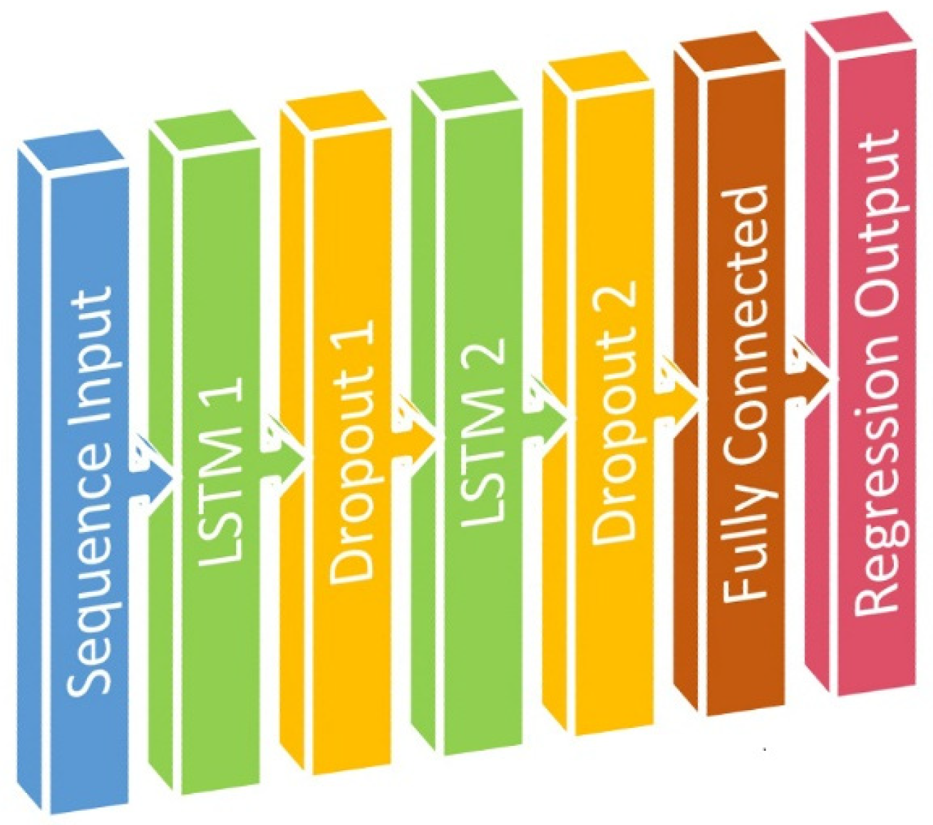
The aerodynamic model at the core of this investigation is a deep sequence-to-sequence regression network. The network is structured as a cascaded pipeline designed specifically for processing temporal data. The network begins with a sequence input layer that accepts 18 input channels, corresponding to the time-history features including the flight and control states. This is followed by two stacked LSTM layers, containing 80 and 60 hidden units, which are designed to capture the long-term temporal dependencies inherent in the unsteady aerodynamic data. To mitigate overfitting and improve generalization, a dropout layer is inserted after each LSTM layer. The final layers consist of a fully connected layer that reduces the feature space to 6 output channels, and a regression output layer that computes the final prediction of the aerodynamic coefficients. The network contains a total of 69,000 learnable parameters, balancing model capacity with computational efficiency for dynamic system identification. The architecture of the employed network is shown in Figure 7.
Figure 7.
The architecture of the employed network.
This architecture is particularly well-suited for the objectives of this paper for several reasons. First, the LSTM layers are specifically designed to model sequential data, making them ideal for capturing the time-dependent, unsteady aerodynamic effects that characterize post-stall maneuvers. Unlike traditional gray-box methods that rely on pre-defined mathematical structures, this deep network can autonomously discover and learn the complex, nonlinear relationships between past inputs and current aerodynamic states directly from flight data. The sequence-to-sequence configuration enables the model to map an entire input time series to an output time series, effectively performing dynamic identification without requiring an explicit state-space representation. Furthermore, the inclusion of dropout layers addresses a key concern in data-driven modeling by helping to ensure that the learned dynamics generalize to unseen maneuvers, rather than simply memorizing the training data.
To develop and rigorously evaluate the LSTM-based black-box identifier, the available time-series data is partitioned into three distinct subsets: 80% for training, 10% for validation, and 10% for testing. This partitioning is essential for developing a model that not only fits the training data but also generalizes effectively to unseen flight conditions, which is particularly critical given the complex and nonlinear nature of post-stall aerodynamics. The training set, comprising the majority of the data, is used to update the network’s 69,000 learnable parameters through backpropagation, allowing the network to learn the underlying input-output relationships. The validation set plays a crucial diagnostic role during the training process; after a specified number of epochs, the model’s performance on this unseen data is monitored to detect the onset of overfitting and to guide hyperparameter tuning. The test set is held back entirely until training is complete, at which point it provides an unbiased, final evaluation of the model’s predictive accuracy on data it has never encountered. The specific split of 80/10/10 is widely accepted in the machine learning community as a standard practice that balances several competing needs. The 80% training allocation provides a sufficiently large and diverse dataset for the LSTM to capture the complex, time-dependent aerodynamic phenomena characteristic of post-stall maneuvers. Simultaneously, the 10% validation and 10% test splits are adequate to provide statistically meaningful estimates of model performance without starving the training process of valuable data, ensuring a robust and credible comparison against the gray-box identification methods.
All training and evaluation were performed on a workstation equipped with an NVIDIA RTX 3050 GPU (4 GB VRAM), an Intel Core i7-10800H CPU @ 2.30 GHz, and 16 GB of RAM. The operating system was Windows 11 Pro. The LSTM network was implemented using MATLAB 2022a with the Deep Learning Toolbox. GPU acceleration was enabled using the Parallel Computing Toolbox with CUDA support. Data preprocessing and postprocessing were conducted using MATLAB’s built-in functions. A fixed random seed (rng(42) in MATLAB) was set before training to ensure reproducibility of results.
In this paper, the Adam algorithm is used for updating the parameters of the aerodynamic model. Adam, derived from adaptive moment estimation, is an optimization algorithm that enhances gradient descent by adapting the learning rate for each parameter and incorporating momentum to accelerate convergence. It maintains two key moving averages: the first moment which tracks the mean of the gradients (providing momentum), and the second moment , which tracks the uncentered variance (the squared gradients) to scale the learning rates individually for each parameter. These are computed using decay rates (Gradient Decay Factor) and (Squared Gradient Decay Factor), as follows [36]:
The parameters are then updated by combining these moments, where the gradient is effectively replaced by the momentum term and normalized by the square root of the second moment:
The learning rate multiplies the normalized update direction, scaling the overall magnitude of the change applied to the parameters. This mechanism allows parameters with large gradients to have their learning rates effectively reduced, while those with small gradients see an increase, all while maintaining directional momentum from recent gradients. A small constant prevents division by zero. The needed parameters of the learning algorithm are presented in Table 1.
Table 1.
The parameters of the model.
6. Results and Discussion
6.1. The First Dataset
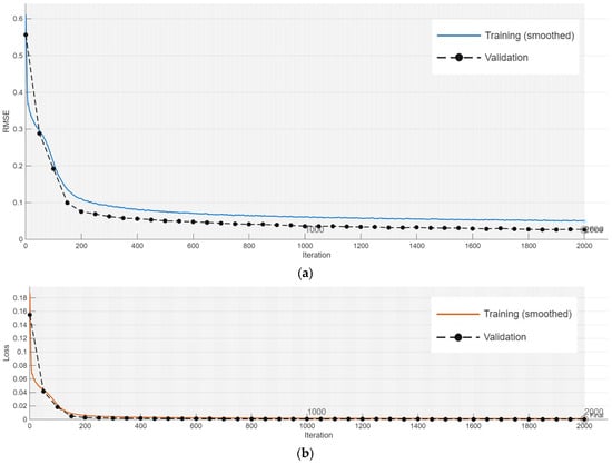
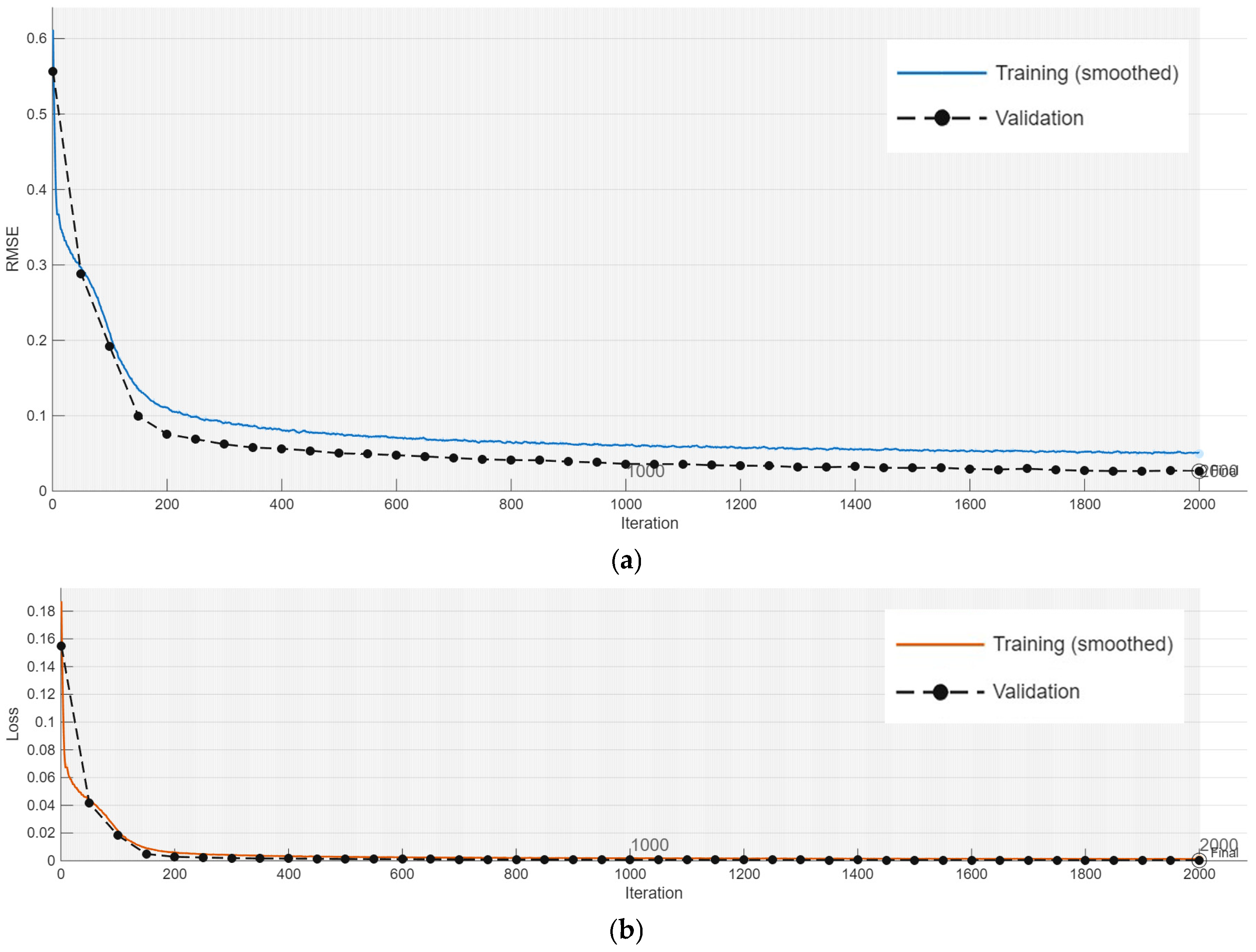
The first dataset is utilized for training the aerodynamic model, as well as validation, and test. The training progress plots are illustrated in Figure 8.
Figure 8.
The training progress plots: (a) RMSE, and (b) loss function.
These plots show the root-mean-square error (RMSE) and loss function, as defined in the following equations:
where and are the sequence length and number of response, respectively.
The plots provide valuable insight into the learning dynamics of the LSTM network over the course of 2000 epochs. The first plot displays the training RMSE against each iteration, alongside the validation RMSE at 50-iteration intervals. The lower plot presents the loss function with the same training and validation trajectories. Several key observations can be made from these profiles. First, both metrics converge rapidly within the first 200 iterations indicating that the network quickly learns the dominant dynamic patterns in the aerodynamic data. Thereafter, both learning curves transition into a prolonged period of gradual refinement, slowly decreasing to a final training RMSE of 0.0465 and a commensurately low loss value. This asymptotic convergence suggests that the learning rate is appropriately configured, allowing for stable optimization without oscillatory behavior or premature stagnation. Critically, the validation metrics closely track their training counterparts throughout the entire process, with no evidence of divergence or upward trend in the later epochs. This close alignment confirms that the network is learning generalizable features of the unsteady aerodynamics rather than simply memorizing the training sequences. The convergence is particularly significant, as the low error magnitude demonstrates that the LSTM network can predict the aerodynamic coefficients with high fidelity. In the context of post-stall aerodynamic modeling, where complex nonlinear phenomena inherently introduce some level of unpredictability, achieving an RMSE on the order of 1 × 10⁻² represents an acceptable and practically useful level of accuracy for dynamic identification, providing confidence in its ability to serve as a robust black-box comparator against the gray-box methods.
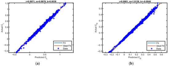
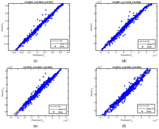
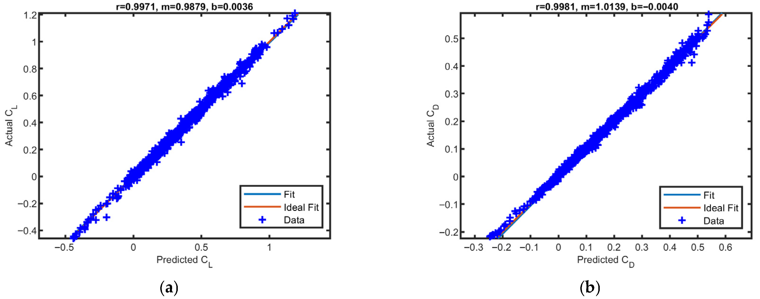
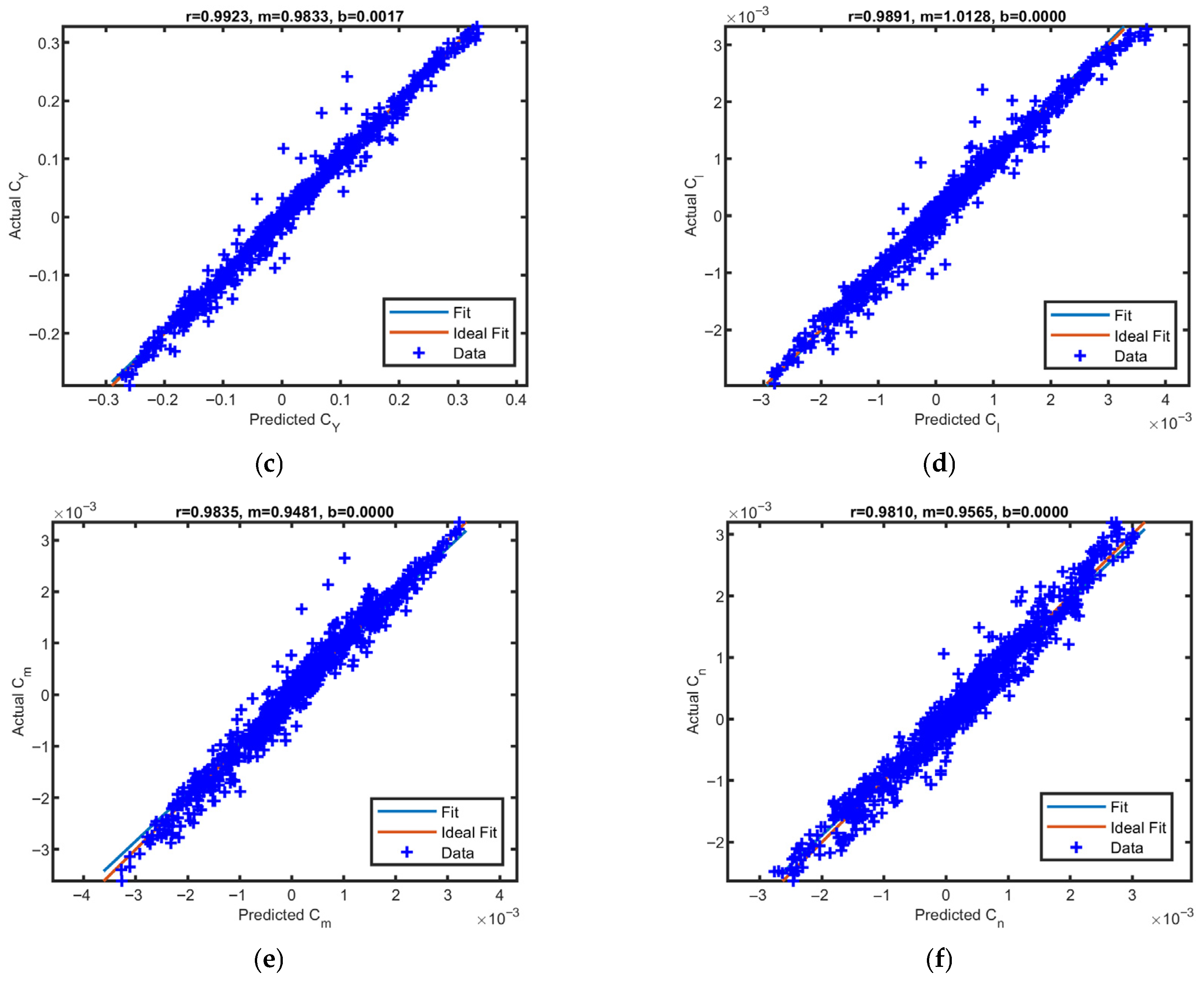
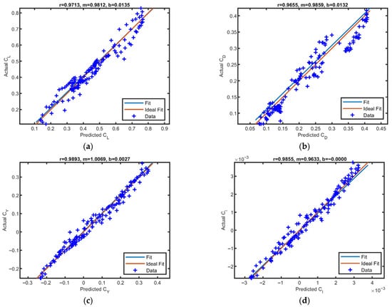
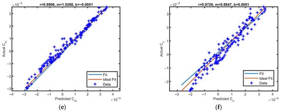
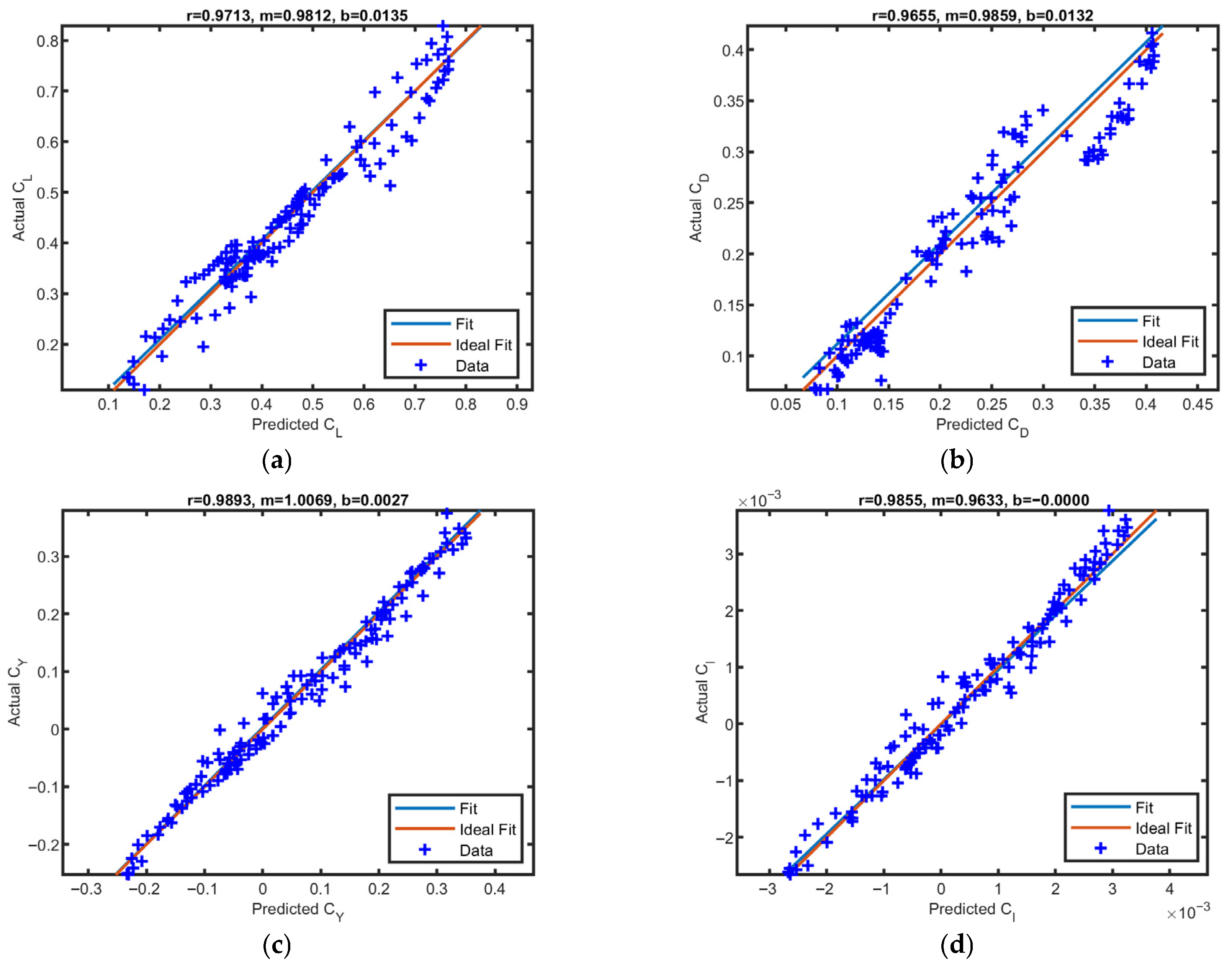
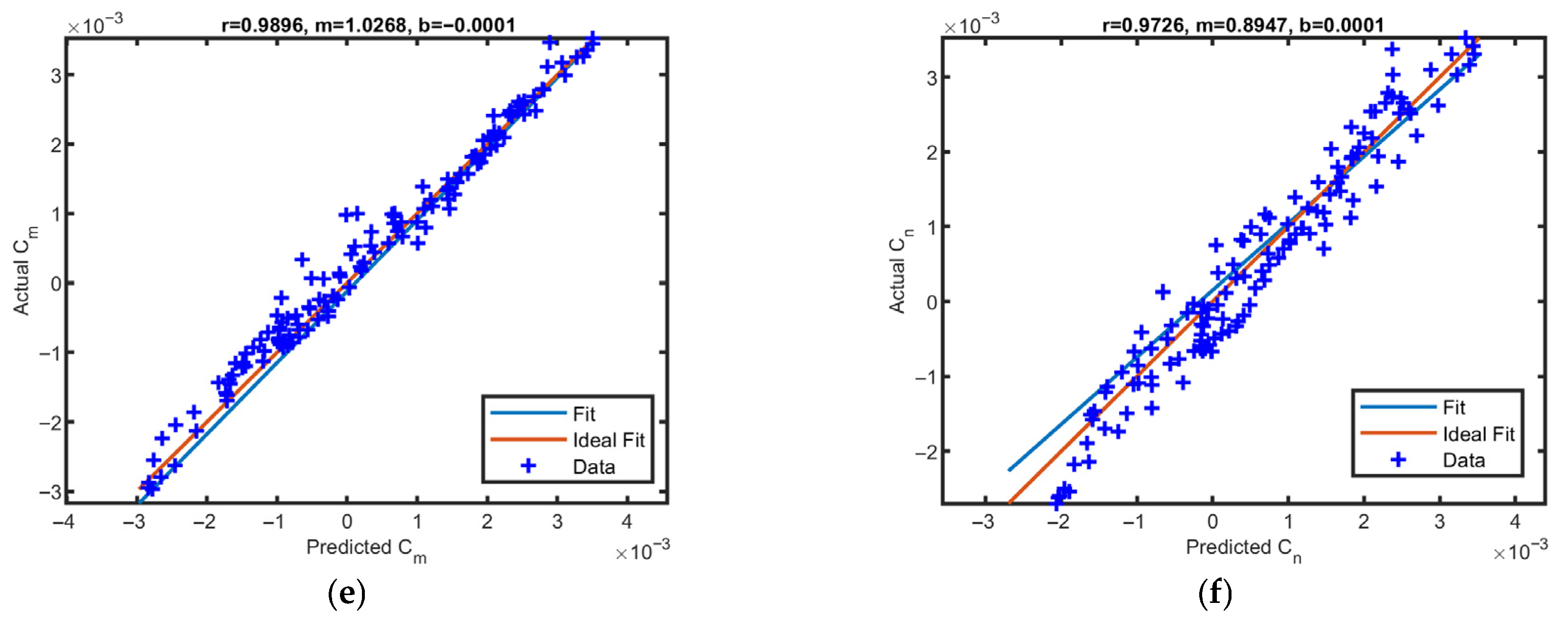
The regression plots for the training phase are illustrated in Figure 9. Also, the regression plots for the test phase are shown in Figure 10. These plots visually represent the relationship between the predicted values and the actual values during the training and test phases. Specifically, a strong regression plot exhibits predictions closely aligned with observed data, indicating that the model has effectively learned the underlying patterns. Key aspects to observe include the distribution of data points around the regression line; a tight clustering signifies higher accuracy, while a wide scatter suggests greater variability and potential for improvement in the model’s predictive capabilities. Deviations from the regression line can also highlight areas where the model struggles to capture complex relationships or suffers from overfitting.
Figure 9.
The regression plots for the training phase: (a) lift coefficient, (b) drag coefficient, (c) side force coefficient, (d) rolling moment coefficient, (e) pitching moment coefficient, (f) yawing moment coefficient.
Figure 10.
The regression plots for the test phase: (a) lift coefficient, (b) drag coefficient, (c) side force coefficient, (d) rolling moment coefficient, (e) pitching moment coefficient, (f) yawing moment coefficient.
The regression, slope, and bias values of the regression plots for the training and test phases are summarized in Table 2. As the comprehensive analysis demonstrates, the results reveal a highly effective regression model, as evidenced by its performance across the training and testing phases for all coefficients. The regression values, consistently approaching 1.0 (ranging from 0.9810 to 0.9981 in training and 0.9655 to 0.9896 in testing), strongly suggest that the model has adeptly captured the intricate relationships inherent in the data. This high degree of correspondence for the test dataset implies an excellent fit and robust generalization capabilities to new, unseen data. A particularly commendable aspect of this model’s performance lies in its bias metrics. The bias values are uniformly minuscule, hovering very close to zero across nearly all coefficients and both phases. This near-elimination of systematic error is a critical hallmark of a high-quality regression, ensuring that predictions are, on average, centered accurately around the true observed values without any consistent overestimation or underestimation bias. While the slope values present a slight degree of variability, with some coefficients showing slopes marginally above or below the ideal value of 1.0, these deviations are generally minor. They indicate that the predicted outcomes are scaling in a manner closely aligned with the actual data, avoiding substantial distortions in magnitude. The remarkable consistency of these strong regression values, negligible bias, and acceptable slope figures, maintained identically in both the training and testing environments, underscores the model’s reliability, accuracy, and its capacity to perform exceptionally well even on data it has not encountered during its learning phase, thereby confirming it as a superior regression solution for these coefficients.
Table 2.
The regression, slope, and bias values [with 95% confidence intervals] of the regression plots for the training and test phases.
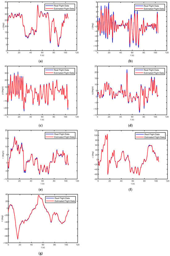
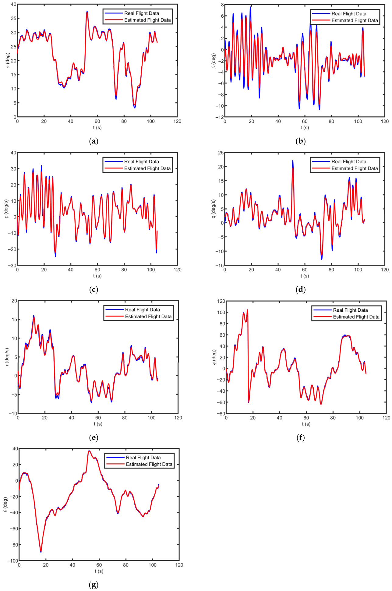
Comparisons are made between the real flight data and the flight parameters estimated by means of the inverse equations of motion from the calculated force and moments in Figure 11.
Figure 11.
Comparisons between the real and estimated flight data for the first dataset: (a) angle of attack, (b) sideslip angle, (c) roll rate, (d) pitch rate, (e) yaw rattabe, (f) bank angle, and (g) pitch angle.
To quantitatively assess the fidelity of the proposed LSTM-based gray-box method, the error statistics between the real flight data and the parameters estimated are computed. The root-mean-square error (RMSE), mean of error (ME), and standard deviation of error (SDE) for the seven key flight variables—angle of attack, sideslip angle, roll rate, pitch rate, yaw rate, bank angle, and pitch angle—are presented in Table 3. These metrics reveal that the model achieves high predictive accuracy for the training dataset. The RMSE values for the angular rates remain below 1.1 deg/s, while the angle of attack and sideslip angle errors are under 0.7 deg. Furthermore, the mean errors (ME) are consistently close to zero, indicating the absence of significant systematic bias. The standard deviations closely track the RMSE values, suggesting that the errors are primarily due to random, zero-mean fluctuations rather than structured inaccuracies. This level of performance on the training data confirms that the LSTM network has successfully captured the dominant nonlinear and unsteady aerodynamic characteristics of the post-stall maneuvers.
Table 3.
The error between the real and estimated flight parameters for the first dataset.
To evaluate model robustness and reduce dependency on a single train-test split, 5-fold cross-validation was performed on the first dataset. The data were partitioned into five equal segments; each fold used four segments for training and the remaining segment for validation. Table 4 reports the mean RMSE across the five folds for the six aerodynamic coefficients.
Table 4.
The 5-fold cross-validation results (mean RMSE ± standard deviation).
The sensitivity of model performance to key hyperparameters was analyzed by varying one parameter at a time while holding others at their nominal values (LSTM layers: 80/60 units; learning rate: 0.001; dropout: 0.2). Table 5 summarizes the results.
Table 5.
Sensitivity analysis: RMSE for under hyperparameter variation.
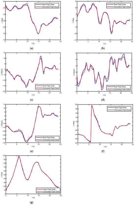
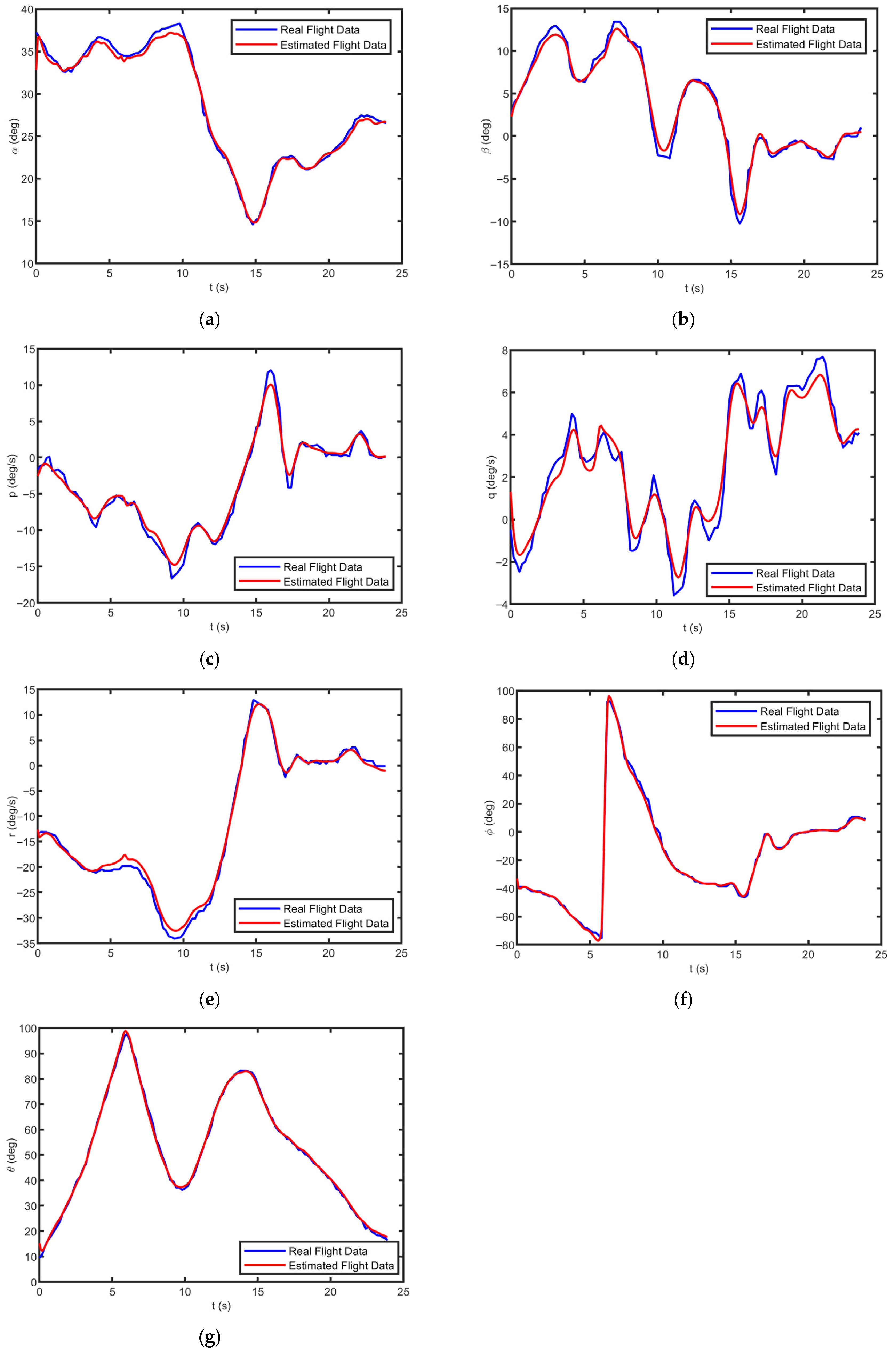
6.2. The Second Dataset
The generalization capability of the LSTM-based gray-box identifier is critically evaluated using the second, completely unseen flight test dataset. The qualitative comparisons presented in Figure 12 provide strong evidence for the model’s generalization capability on the second (unseen) flight dataset. Across all seven flight parameters, the estimated time histories (depicted as red lines) closely track the real flight data (blue lines) despite the complex, nonlinear nature of the post-stall maneuvers. The angle of attack response is captured with particular fidelity, with the model correctly reproducing both the primary excursions and the finer oscillatory features. The sideslip angle, roll rate and yaw rate also show excellent agreement, with only minor phase shifts and amplitude discrepancies occurring during the most aggressive transient regions. The pitch rate estimations, while exhibiting slightly larger deviations during the maneuver’s most extreme segments, still preserve the overall trend and magnitude. These comparisons confirm that the LSTM-based gray-box identifier does not merely memorize the training sequences but has learned the underlying unsteady aerodynamic relationships that govern the aircraft’s motion. The close alignment between real and estimated responses in Figure 12, even for a completely withheld dataset, demonstrates that the model successfully extrapolates to new flight conditions, a critical requirement for practical applications such as flight simulation, control law validation, and envelope expansion.
Figure 12.
Comparisons between the real and estimated flight data for the second dataset: (a) angle of attack, (b) sideslip angle, (c) roll rate, (d) pitch rate, (e) yaw rate, (f) bank angle, and (g) pitch angle.
Table 6 summarizes the error statistics (RMSE, SDE, and ME) between the real flight parameters and those estimated from the network’s predictions on this withheld data. While a slight increase in error magnitudes is observed compared to the training dataset, the overall performance remains remarkably robust. The RMSE for angle of attack is 0.5552 deg. and for sideslip angle it is 0.6235 deg. both of which are still within practically acceptable limits for post-stall aerodynamic identification. The angular rates show RMSE values ranging from 0.5636 deg/s for pitch rate to 0.9180 deg/s for yaw rate, demonstrating that the network preserves its ability to track temporal dynamics without significant degradation. Importantly, the mean errors remain small in magnitude (e.g., 0.0105 for sideslip, −0.0103 for pitch rate), confirming that no substantial bias has been introduced. The close alignment between RMSE and SDE across all variables further indicates that the errors are random and unbiased. This successful performance on the second dataset, without any retraining or fine-tuning, proves that the LSTM network has learned physically consistent, generalizable features of the unsteady aerodynamics rather than simply overfitting to the training sequences. Consequently, the proposed gray-box identifier demonstrates reliable extrapolation capability for complex, multi-degree-of-freedom post-stall maneuvers.
Table 6.
The error between the real and estimated flight parameters for the second dataset.
6.3. Quantitative Comparison with Baseline Models
To rigorously evaluate the advantages of the proposed LSTM-driven gray-box architecture, we compare its performance against two representative baseline models:
- Baseline 1 is a standard Physics-Informed Neural Network (PINN) that incorporates the rigid-body equations only as soft constraints in the loss function. The PINN baseline consists of a feedforward neural network with three hidden layers (128, 96, and 64 neurons) and tanh activations, receiving the instantaneous state and control inputs. The loss function combines mean squared error on aerodynamic coefficients with physics-based penalty terms derived from the residual of equations of motion.
- Baseline 2 is a conventional black-box LSTM model that maps the input regressors directly to outputs without preserving any physical structure. The black-box LSTM baseline uses the same two-layer stacked LSTM architecture (80 and 60 hidden units) as the proposed method but differs fundamentally in its output: rather than predicting aerodynamic coefficients, it directly predicts the flight parameters. No physical constraints are enforced, and the network learns the entire dynamics from scratch.
Table 7 shows the RMSE for the seven reconstructed flight parameters on the unseen second dataset.
Table 7.
The RMSE of the proposed method in comparison with baselines.
The proposed method consistently achieves the lowest prediction errors across all seven flight parameters. Notably, for angular rates (roll, pitch, yaw), the proposed method’s RMSE is approximately 40–60% lower than the black-box LSTM and 60–70% lower than the PINN. This superior performance is attributed to two factors: (1) the hard-coded physical constraints ensure that the predicted states remain dynamically consistent, preventing error accumulation over time; and (2) the LSTM’s gating mechanisms capture the historical dependencies essential for post-stall hysteresis, whereas the PINN’s feedforward architecture with soft constraints cannot adequately represent temporal effects.
As can be seen, the PINN baseline performs worst among the three models, despite incorporating physical knowledge. This counterintuitive result is explained by two factors. First, the PINN’s soft constraint approach allows physics violations during training, and the penalty weight required careful tuning to balance data fit and physical consistency; suboptimal weights led to either poor data fit (high weight) or unphysical predictions (low weight). Second, the feedforward PINN architecture lacks explicit temporal modeling, treating each time step independently. This is fundamentally inadequate for post-stall unsteady aerodynamics, where aerodynamic loads depend critically on flow history. The black-box LSTM baseline, while capturing temporal dependencies, suffers from the absence of physical structure. Only the proposed LSTM-gray architecture combines temporal learning with hard-coded physical constraints, achieving both high accuracy and physical consistency.
Beyond prediction accuracy, the computational requirements of each model are compared. The proposed model requires 28 min of training time on the previously mentioned hardware, which is approximately double that of Baseline 2 (13 min) and triple that of Baseline 1 (8 min). This increased training cost is attributed to the additional forward pass through the inverse dynamics equations at each time step, which must be computed before the loss can be evaluated. GPU memory usage during training peaks at 1.5 GB for the proposed method, 1.2 GB for the black-box LSTM, and 2.2 GB for the PINN. The higher memory consumption of the PINN is due to the need to retain computational graphs for physics loss backpropagation. Overall, while the proposed method incurs higher training costs than the baselines, its superior predictive accuracy and acceptable inference speed justify this trade-off for offline model development. For applications where training time is critical, the black-box LSTM offers a faster but less accurate alternative.
7. Conclusions
This paper presented a gray-box system identification framework for aircraft operating in the challenging post-stall regime, where conventional aerodynamic models fail due to massive flow separation, vortex breakdown, and unsteady hysteresis. By embedding a Long Short-Term Memory (LSTM) network into the physical model representation of aircraft dynamics, the proposed approach preserves the interpretability of first-principles models while leveraging the temporal learning capabilities of deep recurrent architectures. Unlike purely black-box methods that sacrifice physical meaning, this LSTM-driven gray-box identifier maintains the rigid-body equations of motion and uses the network exclusively to learn the uncertain, nonlinear aerodynamic force and moment coefficients directly from flight data.
The framework was developed and rigorously validated using real flight test data from a large-scale (3/8) remotely piloted fighter aircraft, with angles of attack reaching up to 80° during post-stall maneuvers. A sequence-to-sequence LSTM network comprising two stacked layers (80 and 60 hidden units) and approximately 69,000 learnable parameters was trained on the first dataset, with an 80/10/10 split for training, validation, and testing. The second, completely unseen dataset was reserved exclusively for evaluating generalization capability.
Quantitatively, the model achieved exceptional predictive accuracy. The regression coefficients for the six aerodynamic coefficients ranged from 0.9810 to 0.9981 during training and from 0.9655 to 0.9896 during testing, as summarized in Table 2. The bias values remained near zero across all coefficients and both phases, confirming the absence of systematic error. The slope values, while showing minor deviations from the ideal value of 1.0 (e.g., 0.9481 for pitching moment in training, 0.8947 for yawing moment in testing), indicated that predicted outcomes scaled in close alignment with actual data.
For the reconstructed flight parameters on the training dataset, the RMSE values were 0.4485° for angle of attack, 0.6984° for sideslip angle, and 1.0847 deg/s, 0.5901 deg/s, and 0.4602 deg/s for roll, pitch, and yaw rates, respectively. The mean errors (ME) were consistently close to zero, including 0.0048 for sideslip angle and 0.0110 for yaw rate, demonstrating no significant systematic bias. On the unseen second dataset, the model maintained robust performance, with RMSE values of 0.5552° for angle of attack, 0.6235° for sideslip angle, and angular rate errors ranging from 0.5636 deg/s (pitch rate) to 0.9180 deg/s (yaw rate). Although a modest increase in error magnitudes was observed, the mean errors remained small (e.g., 0.0105 for sideslip, −0.0103 for pitch rate), and the close alignment between RMSE and standard deviation confirmed that errors were random and unbiased.
Qualitatively, the time-history comparisons demonstrated that the estimated flight parameters closely tracked the real flight data, capturing both primary excursions and finer oscillatory features even during the most aggressive transient regions of the post-stall maneuvers. The training progress plots showed rapid convergence within the first 200 iterations, with validation metrics closely tracking training metrics throughout all 2000 epochs, confirming that the network learned generalizable features rather than memorizing the training sequences.
In summary, the LSTM-driven gray-box identification framework successfully balances accuracy, physical interpretability, and extrapolation reliability. The near-zero bias, high regression coefficients, and robust performance on unseen data demonstrate that the network has learned physically consistent, time-dependent aerodynamic relationships. This methodology offers a practical and scalable solution for aerodynamic model identification in aggressive flight regimes, with direct applications in flight simulation, envelope expansion, control law validation, and the design of next-generation agile aircraft. Future work may extend this framework to incorporate online adaptive learning, multi-fidelity data fusion, and real-time implementation for flight control systems.
Several limitations of the current study must be acknowledged. First, the method assumes a rigid aircraft with perfect XZ-plane symmetry, no propulsive effects, and a static atmosphere, neglecting aeroelastic coupling, thrust dynamics, and turbulence. Second, validation was conducted on only two flight datasets from a single aircraft configuration (3/8-scale fighter); generalization to other aircraft types and flight regimes remains unproven. Third, the LSTM requires substantial training data (approximately 10,000 time steps), and performance on sparse data has not been evaluated. Fourth, direct quantitative comparison with classical and hybrid methods was not performed. Future work will address these limitations through: (1) validation on benchmark datasets to enable cross-study comparison; (2) transfer learning to reduce data requirements; (3) model compression (pruning, quantization) targeting inference for real-time deployment; and (4) hardware-in-the-loop validation on embedded platforms.
Funding
This research received no external funding.
Data Availability Statement
The original contributions presented in this study are included in the article. Further inquiries can be directed to the corresponding author.
Conflicts of Interest
The author declares no conflict of interest.
Nomenclature
| Symbol | Definition |
| Wing span | |
| Bias vector | |
| Mean aerodynamic chord | |
| Cell state vectors | |
| Force coefficients in stability frame | |
| Moment coefficients in body frame | |
| Input gate, forget gate, cell candidate, and output gate | |
| Gravity acceleration | |
| Altitude | |
| Hidden state vectors | |
| Moments of inertia | |
| Aircraft mass | |
| Momentum term | |
| Rotational velocity components in body frame | |
| Dynamic pressure | |
| Number of response | |
| Recurrent weights | |
| Wing reference area | |
| Sequence length | |
| Time step | |
| Control input vector | |
| Translational velocity components in body frame | |
| Total velocity | |
| Second moment | |
| Input weights | |
| Input data | |
| State vector | |
| Learning rate | |
| Angle of attack | |
| Sideslip angle | |
| Gradient Decay Factor | |
| Squared Gradient Decay Factor | |
| Elevator, aileron and rudder control commands | |
| Euler angles | |
| State activation function | |
| Model parameters | |
| Small constant preventing division by zero |
References
- Mazhar, M.F.; Ahmad, J.; Shafi, I.; Wasim, M.; Abbas, M.; Ashraf, I. Advanced Practices in Aircraft System Identification: Perspective Evaluation and Practical Implementation Schemes. Int. J. Aeronaut. Space Sci. 2025, 27, 1950–1976. [Google Scholar] [CrossRef] [Scilit]
- Tischler, M.B. System identification methods for aircraft flight control development and validation. In Advances in Aircraft Flight Control; NASA: Washington, DC, USA, 2018; pp. 35–69. [Google Scholar]
- Goman, M.; Khrabrov, A. State-space representation of aerodynamic characteristics of an aircraft at high angles of attack. J. Aircr. 1994, 31, 1109–1115. [Google Scholar] [CrossRef] [Scilit]
- Mi, B.G.; Zhan, H.; Lu, S.S. An extended unsteady aerodynamic model at high angles of attack. Aerosp. Sci. Technol. 2018, 77, 788–801. [Google Scholar] [CrossRef] [Scilit]
- Ghoreyshi, M.; Cummings, R.M. Unsteady aerodynamic modeling of aircraft control surfaces by indicial response methods. AIAA J. 2014, 52, 2683–2700. [Google Scholar] [CrossRef] [Scilit]
- Fan, Y.; Lutze, F. Identification of an unsteady aerodynamic model at high angles of attack. In Proceedings of the 21st Atmospheric Flight Mechanics Conference, San Diego, CA, USA, 29–31 July 1996; p. 3407. [Google Scholar]
- Senlin, C.H.; Zhenghong, G.A.; Xinqi, Z.H.; Yiming, D.U.; Chao, P.A. Unstable unsteady aerodynamic modeling based on least squares support vector machines with general excitation. Chin. J. Aeronaut. 2020, 33, 2499–2509. [Google Scholar] [CrossRef] [Scilit]
- Wang, Q.; Qian, W.; He, K. Unsteady aerodynamic modeling at high angles of attack using support vector machines. Chin. J. Aeronaut. 2015, 28, 659–668. [Google Scholar] [CrossRef] [Scilit]
- Alkhedher, M. Comparative study of machine learning modeling for unsteady aerodynamics. Comput. Mater. Contin. 2022, 72, 1901. [Google Scholar] [CrossRef] [Scilit]
- Yetkin, S.; Abuhanieh, S.; Yigit, S. Investigation on the abilities of different artificial intelligence methods to predict the aerodynamic coefficients. Expert Syst. Appl. 2024, 237, 121324. [Google Scholar] [CrossRef] [Scilit]
- Mi, B.; Cheng, S.; Zhan, H.; Yu, J.; Wang, Y. Development on Unsteady Aerodynamic Modeling Technology at High Angles of Attack. Arch. Comput. Methods Eng. 2024, 31, 4305–4357. [Google Scholar] [CrossRef] [Scilit]
- Ignatyev, D.I.; Khrabrov, A.N. Neural network modeling of unsteady aerodynamic characteristics at high angles of attack. Aerosp. Sci. Technol. 2015, 41, 106–115. [Google Scholar] [CrossRef] [Scilit]
- Li, K.; Kou, J.; Zhang, W. Deep neural network for unsteady aerodynamic and aeroelastic modeling across multiple Mach numbers. Nonlinear Dyn. 2019, 96, 2157–2177. [Google Scholar] [CrossRef] [Scilit]
- Kou, J.; Zhang, W. Data-driven modeling for unsteady aerodynamics and aeroelasticity. Prog. Aerosp. Sci. 2021, 125, 100725. [Google Scholar] [CrossRef] [Scilit]
- Suresh, S.; Omkar, S.N.; Mani, V.; Prakash, T.G. Lift coefficient prediction at high angle of attack using recurrent neural network. Aerosp. Sci. Technol. 2003, 7, 595–602. [Google Scholar] [CrossRef] [Scilit]
- Mohan George, S.; Selvi, S.S.; Raol, J.R. Recurrent neural networks for aerodynamic parameter estimation with Lyapunov stability analysis. Syst. Sci. Control Eng. 2024, 12, 2363387. [Google Scholar] [CrossRef] [Scilit]
- Raissi, M.; Perdikaris, P.; Karniadakis, G.E. Physics-informed neural networks: A deep learning framework for solving forward and inverse problems involving nonlinear partial differential equations. J. Comput. Phys. 2019, 378, 686–707. [Google Scholar] [CrossRef] [Scilit]
- Yan, M.; Liu, K.; An, S.; Wang, G.; Jin, Z.; Zang, J. Transfer learning-driven adaptive physics-informed neural networks acceleration method for aerodynamic identification. Eng. Appl. Artif. Intell. 2026, 166, 113589. [Google Scholar] [CrossRef] [Scilit]
- Liu, C.P.; Song, W.P.; Xu, C.Z.; Han, Z.H. Physics-informed data-driven nonlinear unsteady aerodynamic modelling at high angles of attack. Chin. J. Aeronaut. 2025, 12, 103943. [Google Scholar] [CrossRef] [Scilit]
- Wang, X.; Kou, J.; Zhang, W.; Liu, Z. Incorporating physical models for dynamic stall prediction based on machine learning. AIAA J. 2022, 60, 4428–4439. [Google Scholar] [CrossRef] [Scilit]
- Dong, W.; Wang, X.; Lin, Q.; Cheng, C.; Zhu, L. A weighted feature fusion model for unsteady aerodynamic modeling at high angles of attack. Aerospace 2024, 11, 339. [Google Scholar] [CrossRef] [Scilit]
- Ma, J.; Zhu, Q.; Xue, T.; Ai, J.; Dong, Y. Aircraft dynamics modeling at high angle of attack incorporating residual transformer autoencoder and physical mechanisms. Aerosp. Sci. Technol. 2025, 160, 110045. [Google Scholar] [CrossRef] [Scilit]
- Xiong, F.; Zhang, L. A point cloud deep neural network metamodel method for aerodynamic prediction. Chin. J. Aeronaut. 2023, 36, 92–103. [Google Scholar] [CrossRef] [Scilit]
- Xu, B.; Yang, W.; Zhou, Y.; Zhao, W.; Wu, X.; Zhang, Z.; Liu, Y. A data-driven online estimation method for aerodynamic parameter of high-speed aircraft considering strong nonlinearity and noise. ISA Trans. 2025, 163, 86–97. [Google Scholar] [CrossRef] [Scilit]
- Dong, W.; Wang, X.; Han, D.; Lin, Q. Unsteady aerodynamic modeling and analysis of aircraft model in multi-DOF coupling maneuvers at high angles of attack with attention mechanism. Chin. J. Aeronaut. 2025, 38, 103444. [Google Scholar] [CrossRef] [Scilit]
- Marques, F.D.; Anderson, J. Identification and prediction of unsteady transonic aerodynamic loads by multi-layer functionals. J. Fluids Struct. 2001, 15, 83–106. [Google Scholar] [CrossRef] [Scilit]
- Verma, H.O.; Peyada, N.K. Estimation of aerodynamic parameters near stall using maximum likelihood and extreme learning machine-based methods. Aeronaut. J. 2021, 125, 489–509. [Google Scholar] [CrossRef] [Scilit]
- Haizhou, W.U.; Xuejun, L.I.; Wei, A.N.; Hongqiang, L.Y. A generative deep learning framework for airfoil flow field prediction with sparse data. Chin. J. Aeronaut. 2022, 35, 470–484. [Google Scholar] [CrossRef] [Scilit]
- Hou, W.; Darakananda, D.; Eldredge, J.D. Machine-learning-based detection of aerodynamic disturbances using surface pressure measurements. AIAA J. 2019, 57, 5079–5093. [Google Scholar] [CrossRef] [Scilit]
- Xu, D.; Zang, J.; Song, X.Y.; Zhang, Z.; Zhang, Y.W.; Chen, L.Q. Deep learning-enabled explicit dynamics model parameters for composite structures. Int. J. Mech. Sci. 2026, 316, 111472. [Google Scholar] [CrossRef] [Scilit]
- Xu, D.; Zang, J.; Song, X.Y.; Zhang, Z.; Zhang, Y.W.; Chen, L.Q. Uncertain dynamics characteristic forecasting in composite plates with multi-defects of electric aircraft via physics-augmented meta-learning. Aerosp. Sci. Technol. 2025, 164, 110363. [Google Scholar] [CrossRef] [Scilit]
- Zhe, H.U.; Yinan, K.O.; Weigang, Y.A.; Gang, C.H. Aircraft parameter estimation using a stacked long short-term memory network and Levenberg-Marquardt method. Chin. J. Aeronaut. 2024, 37, 123–136. [Google Scholar]
- Bekhiti, B.; Hariche, K.; Zaitsev, V.; Duan, G.R.; Sharkawy, A.N. The Algebraic Theory of Operator Matrix Polynomials with Applications to Aeroelasticity in Flight Dynamics and Control. Math. Comput. Appl. 2025, 30, 131. [Google Scholar] [CrossRef] [Scilit]
- Bekhiti, B.; Hariche, K.; Ma’arif, A.; Sharkawy, A.N. A Nonlinear Automatic Control Strategy for Autopiloting a Fourth-Generation Combat Aircraft: The Soukhoï Su-30. Int. J. Robot. Control Syst. 2025, 5, 2957–2994. [Google Scholar] [CrossRef] [Scilit]
- Holleman, E.C. Summary of Flight Tests to Determine the Spin and Controllability Characteristics of a Remotely Piloted, Large-Scale (3/8) Fighter Airplane Model; NASA Report No. H-889; NASA: Washington, DC, USA, 1976.
- Kingma, D.P.; Ba, J. Adam: A method for stochastic optimization. arXiv 2014, arXiv:1412.6980. [Google Scholar]

Disclaimer/Publisher’s Note: The statements, opinions and data contained in all publications are solely those of the individual author(s) and contributor(s) and not of MDPI and/or the editor(s). MDPI and/or the editor(s) disclaim responsibility for any injury to people or property resulting from any ideas, methods, instructions or products referred to in the content. |
© 2026 by the author. Licensee MDPI, Basel, Switzerland. This article is an open access article distributed under the terms and conditions of the Creative Commons Attribution (CC BY) license.