Modeling Diverse Hazard Shapes with the Power Length-Biased XLindley Distribution
Abstract
1. Introduction
- The development of a novel two-parameter lifetime distribution capable of modeling a wide range of complex hazard rate shapes, including decreasing, increasing, decreasing-increasing-decreasing, and inverted bathtub forms.
- Addressing a notable research gap by proposing a model that maintains analytical tractability while providing greater flexibility compared to existing models.
- A comprehensive mathematical treatment of the proposed model that encompasses its distributional properties, inferential methods, and applications to real-world data.
- Motivated by both theoretical considerations and practical limitations of existing models, the proposed distribution offers a valuable new tool for researchers and practitioners in fields where understanding time-to-event phenomena is essential.
2. PLXL Distribution and Its Statistical Properties
2.1. The PDF and Its Shape
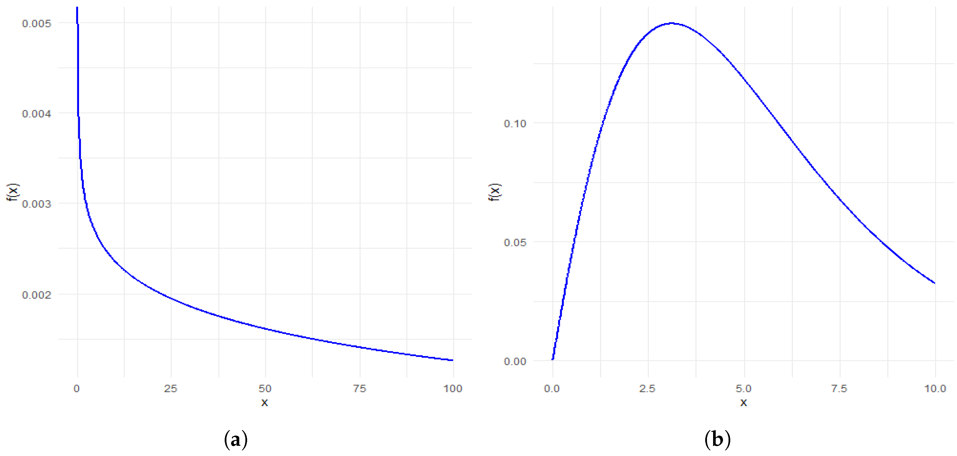
- decreasing if
- (a)
- ,
- (b)
- ;
- unimodal if
- (a)
- ,
- (b)
- .
- (a)
- If or , then , , and are all negative. Hence, for all and the PDF is decreasing.If , then and , and the discriminant , so the roots are complex. Hence, for all , and the PDF is decreasing.
- (b)
- If , then , , and are negative, so the PDF is decreasing.
- (a)
- If , then and . Regardless of the sign of , the coefficients of exhibit exactly one sign change. By Descartes’ Rule of Signs, has exactly one positive root. Also, and . Therefore, changes sign once, and is unimodal.
- (b)
- If , then , , and has one positive real root. Hence, the PDF is unimodal.
- The mode is at zero if
- If , the mode is
- If , the mode is
2.2. The HRF and Its Shapes
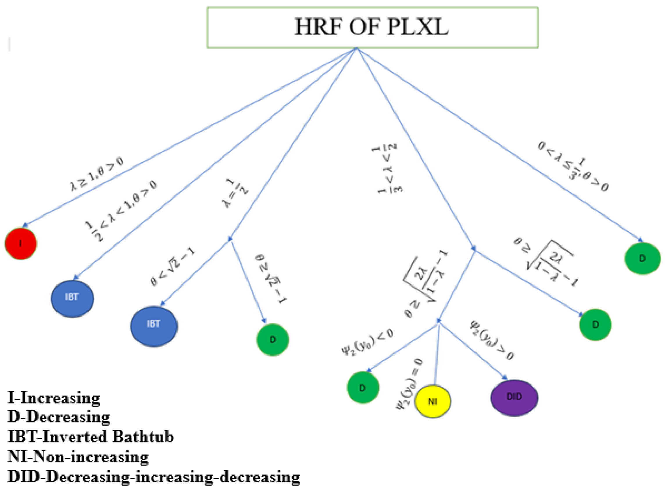
- Decreasing if .
- Non-increasing if .
- Decreasing-increasing-decreasing if .
- (i)
- .
- (ii)
- .
- (iii)
- .
- If , then for all positive y, and hence the HRF is decreasing.
- If , then the HRF is non-increasing since is negative for all positive y except at .
- If , then there should be two positive roots. Since changes direction one time with , we must have decreasing-increasing-decreasing shape for the hazard rate.
2.3. Change Point of the HRF
2.4. Moments of the PLXL Distribution
3. Estimation and Simulation
3.1. ML Estimation
3.2. LS Estimation
3.3. Generating Random Observations
- Generate observations and , , from the GG distributions: and , respectively.
- Generate observations from the uniform distribution over (0, 1).
- If , set ; else, set .
3.4. Comparison of the ML and LS Estimations Using Simulated Observations
- In all the cases, the MSEs of the MLEs and LSEs of both and decrease as sample size increases. This also indicates that the estimators and are consistent.
- In all the cases, the MSEs of the MLEs of both and are lesser than the MSEs of LSEs of and . This shows that the MLEs perform better than the LSEs.
- As sample size increases, the differences in MSE of MLEs and LSEs decrease, indicating that for large sample sizes, the MLEs and LSEs are almost equally efficient.
4. Modeling Right-Censored Data
5. Real-Life Application
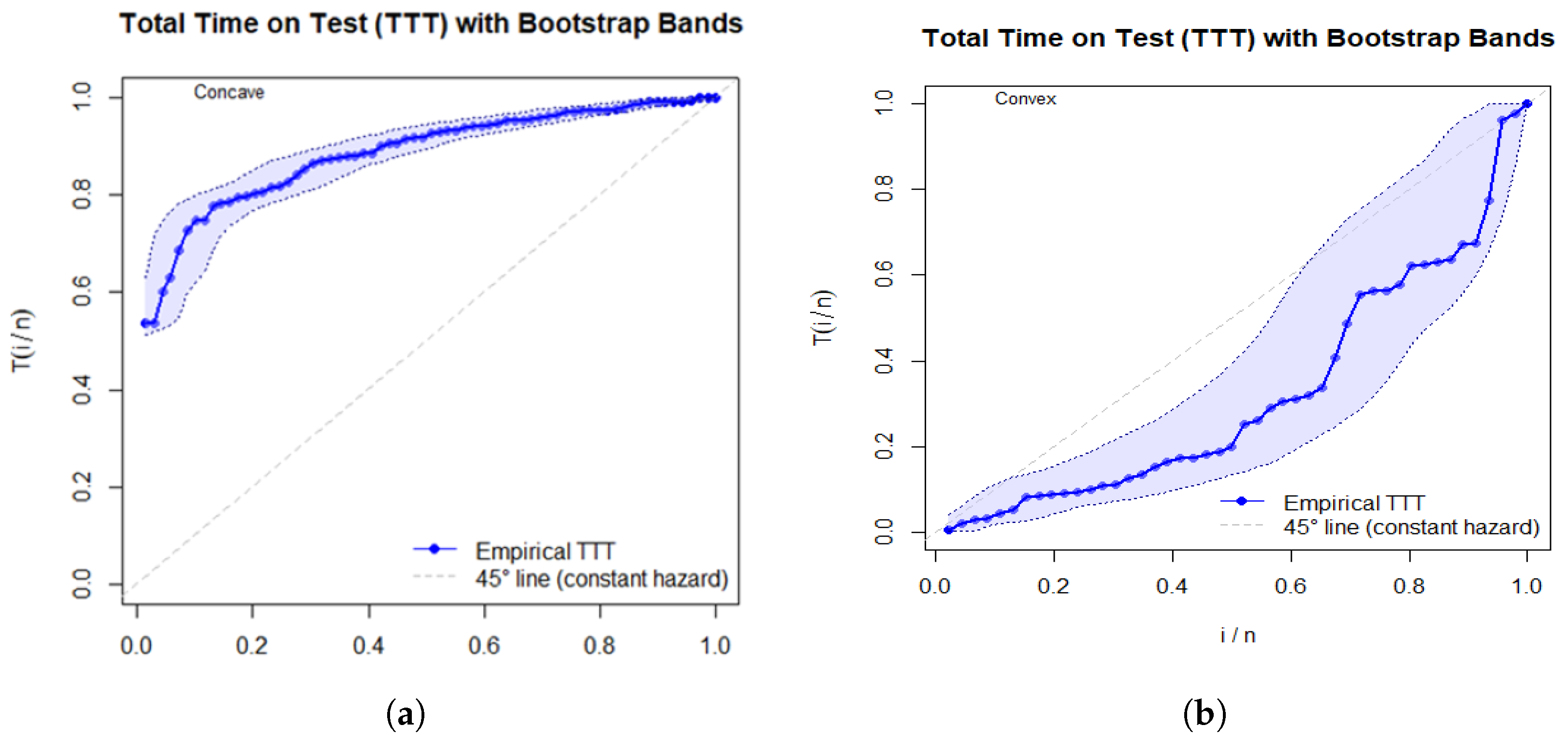
5.1. Modelling Uncensored Data
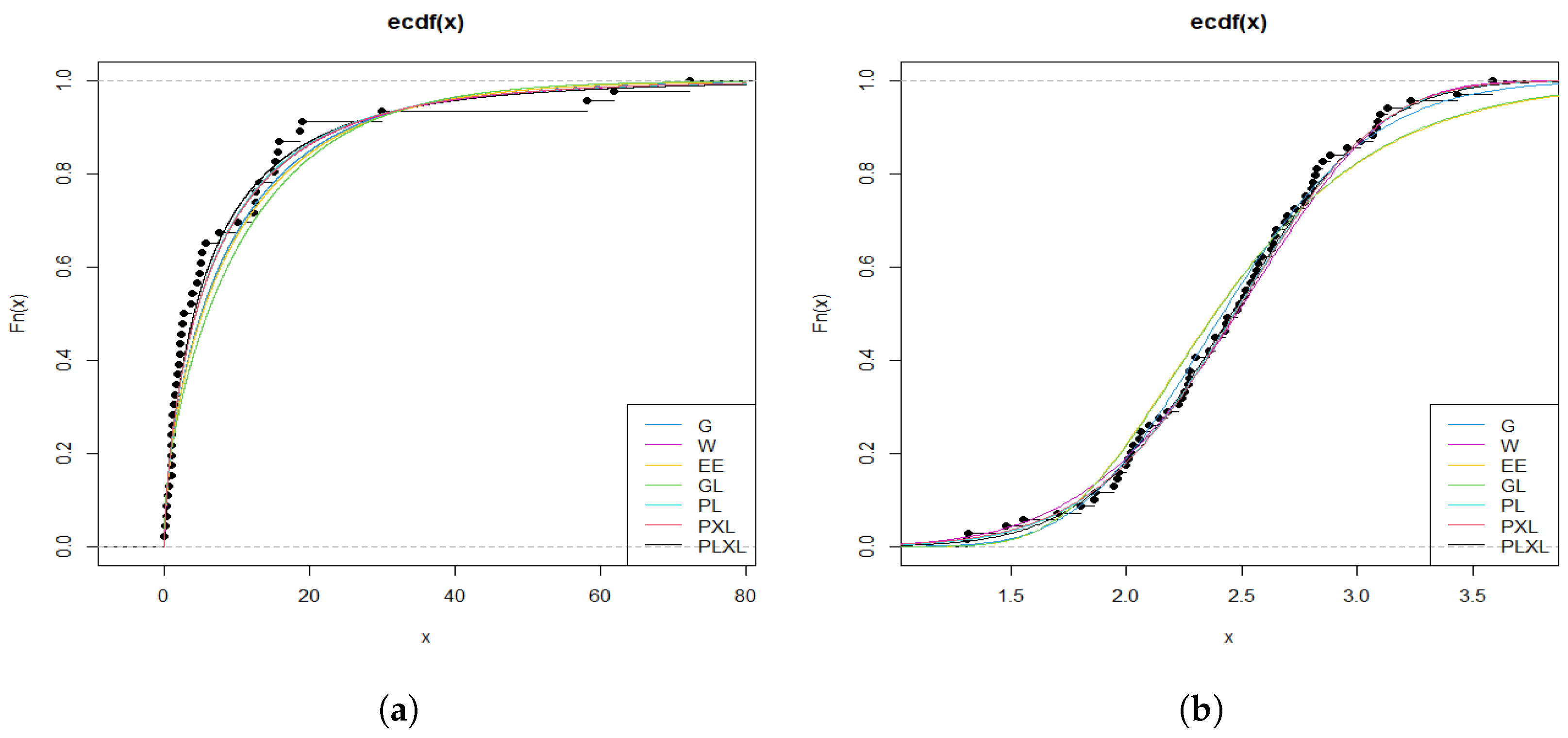
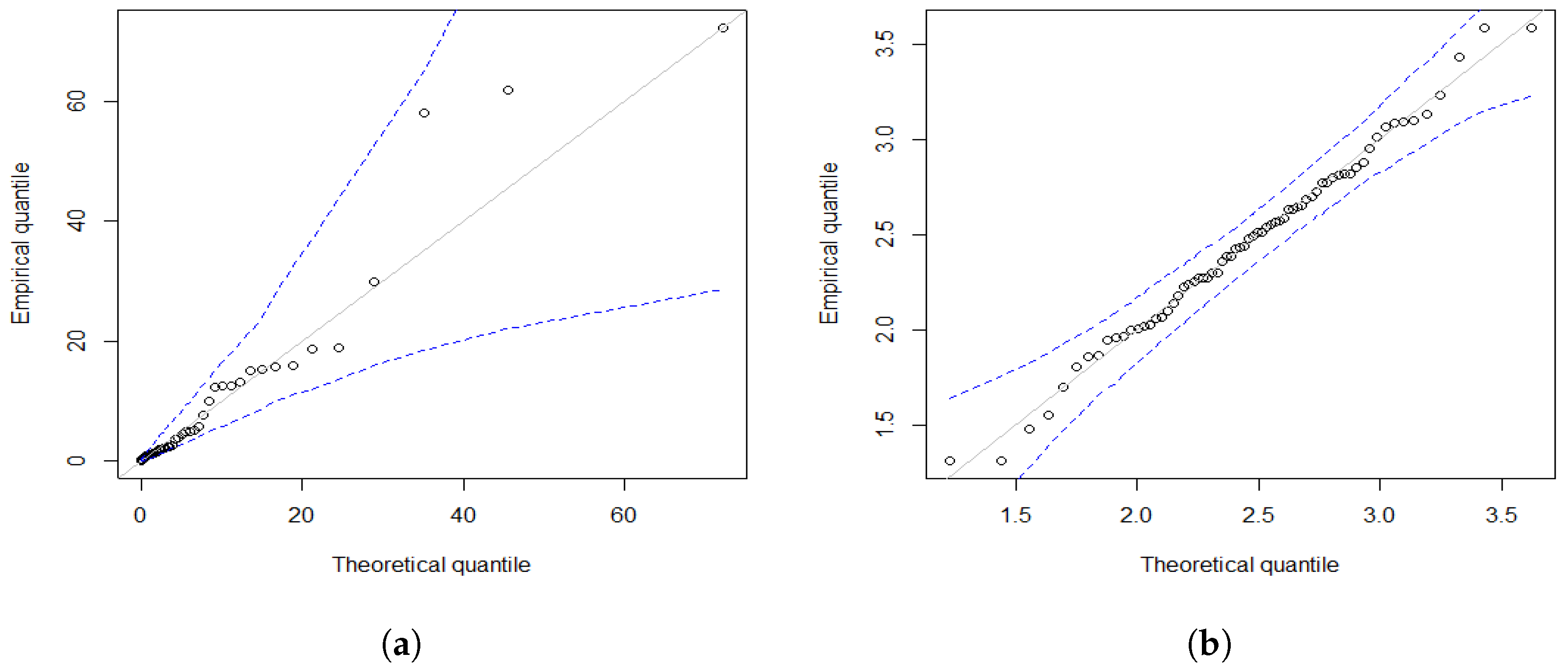
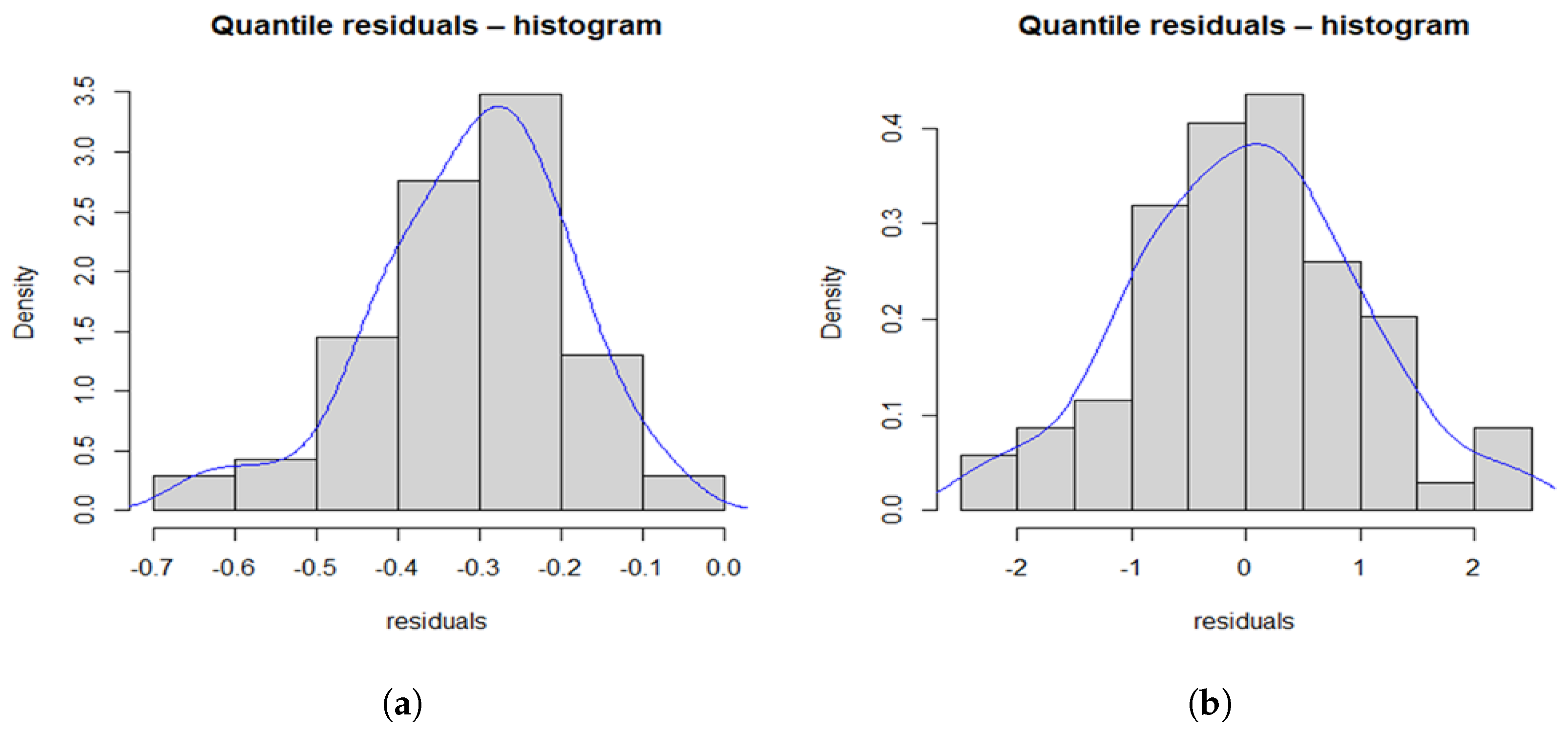
- Data set 1 (Vaccination rates):0.042, 0.205, 0.285, 0.319, 0.464, 0.550, 0.889, 0.895, 0.939, 0.986, 1.000, 1.088, 1.212, 1.244, 1.450, 1.593, 1.844, 2.039, 2.157, 2.167, 2.334, 2.440, 2.657, 3.685, 3.879, 4.493, 4.800, 4.944, 5.155, 5.674, 7.602, 10.004, 12.238, 12.520, 12.553, 13.063, 15.105, 15.229, 15.629, 15.848, 18.641, 18.940, 29.885, 58.162, 61.838, 72.286.
- Data set 2 (Carbon fiber stress):1.312, 1.314, 1.479, 1.552, 1.700, 1.803, 1.861, 1.865, 1.944, 1.958, 1.966, 1.997, 2.006, 2.021, 2.027, 2.055, 2.063, 2.098, 2.140, 2.179, 2.224, 2.240, 2.253, 2.270, 2.272, 2.274, 2.301, 2.301, 2.359, 2.382, 2.382, 2.426, 2.434, 2.435, 2.478, 2.490, 2.511, 2.514, 2.535, 2.554, 2.566, 2.570, 2.586, 2.629, 2.633, 2.642, 2.648, 2.684, 2.697, 2.726, 2.770, 2.773, 2.800, 2.809, 2.818, 2.821, 2.848, 2.880, 2.954, 3.012, 3.067, 3.084, 3.090, 3.096, 3.128, 3.233, 3.433, 3.585, 3.585.
5.2. Modelling Censored Data
- Data set 3 (remission times):4.50, 32.15, 3.88, 13.80, 19.13, 4.87, 3.02*, 5.85, 14.24, 5.71, 19.36*, 7.09, 7.87, 7.59, 20.28, 5.32, 5.49, 46.12, 2.02, 4.51, 5.17, 2.83, 9.22, 1.05, 0.20, 8.37, 3.82, 9.47, 36.66, 14.77, 26.31, 79.05, 10.06, 8.53, 4.65*, 2.02, 4.98, 11.98, 2.62, 4.26, 5.06, 1.76, 0.90, 11.25, 16.62, 4.40, 21.73, 10.34, 12.07, 34.26, 0.87*, 10.66, 6.97, 2.07, 0.51, 12.03, 0.08, 17.12, 3.36, 2.64, 1.40, 12.63, 43.01, 14.76, 2.75, 7.66, 0.81, 1.19, 7.32, 4.18, 3.36, 8.66, 1.26, 13.29, 1.46, 14.83, 6.76, 23.63, 24.80*, 5.62, 8.60*, 3.25, 10.86*, 18.10, 7.62, 7.63, 17.14, 25.74, 3.52, 2.87, 15.96, 17.36, 9.74, 3.31, 7.28, 1.35, 0.40, 2.26, 4.33*, 9.02, 5.41, 2.69, 22.69, 6.94, 2.54, 11.79, 2.46, 7.26, 2.69, 5.34, 3.48, 4.70*, 8.26, 6.93, 4.23, 3.70, 0.50, 10.75, 6.54, 3.64, 5.32, 13.11, 8.65, 3.57, 5.09, 7.39, 5.41, 11.64, 2.09, 2.23, 6.25, 7.93, 4.34, 25.82, 12.02.
6. Conclusions
Author Contributions
Funding
Data Availability Statement
Conflicts of Interest
References
- Efron, B. Logistic regression, survival analysis, and the Kaplan-Meier curve. J. Am. Stat. Assoc. 1988, 83, 414–425. [Google Scholar] [CrossRef]
- Andrews, D.F.; Herzberg, A. Data: A Collection of Problems from Many Fields for the Student and Research Worker; Series in Statistics; Springer: New York, NY, USA, 1985. [Google Scholar]
- Lindley, D.V. Fiducial distributions and Bayes’ theorem. J. R. Stat. Soc. Ser. B 1958, 20, 102–107. [Google Scholar] [CrossRef]
- Ghitany, M.; Al-Mutairi, D.; Balakrishnan, N.; Al-Enezi, L. Power Lindley distribution and associated inference. Comput. Stat. Data Anal. 2013, 64, 20–33. [Google Scholar] [CrossRef]
- Ghitany, M.; Alqallaf, F.; Al-Mutairi, D.K.; Husain, H.A. A two-parameter weighted Lindley distribution and its applications to survival data. Math. Comput. Simul. 2013, 81, 1190–1201. [Google Scholar] [CrossRef]
- Nadarajah, S.; Bakouch, H.; Tahmasbi, R. A generalized Lindley distribution. Sankhya B 2011, 73, 331–359. [Google Scholar] [CrossRef]
- Sharma, V.K.; Singh, S.K.; Singh, U.; Agiwal, V. The inverse Lindley distribution: A stress-strength reliability model with application to head and neck cancer data. J. Ind. Prod. Eng. 2015, 32, 162–173. [Google Scholar] [CrossRef]
- Barco, K.; Mazucheli, J.; Janeiro, V. The inverse power Lindley distribution. Commun. Stat.-Simul. Comput. 2017, 46, 6308–6323. [Google Scholar] [CrossRef]
- Chouia, S.; Zeghdoudi, H. The XLindley distribution: Properties and application. J. Stat. Theory Appl. 2021, 20, 318–327. [Google Scholar] [CrossRef]
- Metiri, F.; Zeghdoudi, H.; Ezzebsa, A. On the characterisation of XLindley distribution by truncated moments. properties and application. Oper. Res. Decis. 2022, 32, 97–109. [Google Scholar]
- Zinhom, E.; Nassar, M.; Radwan, S.; Elmasry, A. The wrapped XLindley distribution. Environ. Ecol. Stat. 2023, 30, 669–686. [Google Scholar] [CrossRef]
- Etaga, H.O.; Nwankwo, M.P.; Oramulu, D.O.; Anabike, I.C.; Obulezi, O.J. The double XLindley distribution: Properties and applications. Sch. J. Phys. Math. Stat. 2023, 10, 192–202. [Google Scholar] [CrossRef]
- Beghriche, A.; Tashkandy, Y.A.; Bakr, M.E.; Zeghdoudi, H.; Gemeay, A.M.; Hossain, M.M.; Muse, A.H. The inverse XLindley distribution: Properties and application. IEEE Access 2023, 11, 47272–47281. [Google Scholar] [CrossRef]
- MirMostafaee, S. The exponentiated new XLindley distribution: Properties, and Applications. J. Data Sci. Model. 2023, 2, 185–208. [Google Scholar]
- Gemeay, A.M.; Ezzebsa, A.; Zeghdoudi, H.; Tanış, C.; Tashkandy, Y.A.; Bakr, M.; Kumar, A. The power new XLindley distribution: Statistical inference, fuzzy reliability, and applications. Heliyon 2024, 10, e36594. [Google Scholar] [CrossRef]
- Alghamdi, F.M.; Ahsan-ul Haq, M.; Hussain, M.N.S.; Hussam, E.; Almetwally, E.M.; Aljohani, H.M.; Mustafa, M.S.; Alshawarbeh, E.; Yusuf, M. Discrete Poisson quasi-XLindley distribution with mathematical properties, regression model, and data analysis. J. Radiat. Res. Appl. Sci. 2024, 17, 100874. [Google Scholar] [CrossRef]
- Alomair, A.M.; Ahmed, M.; Tariq, S.; Ahsan-ul Haq, M.; Talib, J. An exponentiated XLindley distribution with properties, inference and applications. Heliyon 2024, 10, e25472. [Google Scholar] [CrossRef] [PubMed]
- Musekwa, R.R.; Makubate, B. A flexible generalized XLindley distribution with application to engineering. Sci. Afr. 2024, 24, e02192. [Google Scholar] [CrossRef]
- Alsadat, N. A new extension of XLindley distribution with mathematical properties, estimation, and application on the rainfall data. Heliyon 2024, 10, e38143. [Google Scholar] [CrossRef]
- Kouadria, M.; Zeghdoudi, H. The truncated new-XLindley distribution with applications. J. Comput. Anal. Appl. 2025, 34, 53–64. [Google Scholar]
- Wang, X. A simple proof of descartes’s rule of signs. Am. Math. Mon. 2004, 111, 525–526. [Google Scholar] [CrossRef]
- R Core Team. R: A Language and Environment for Statistical Computing; R Foundation for Statistical Computing: Vienna, Austria. 2025. Available online: https://www.R-project.org/ (accessed on 26 August 2025).
- Swain, J.; Venkatraman, S.; Wilson, J. Least squares estimation of distribution function in Johnson’s translation system. J. Stat. Comput. Simul. 2025, 29, 271–297. [Google Scholar] [CrossRef]
- Johnson, N.; Kotz, S.; Balakrishnan, N. Continuous Univariate Distribution; John Wiley: New York, NY, USA, 1995. [Google Scholar]
- Almongy, H.M.; Almetwally, E.; Ahmad, H.; Al-nefaie, A. Modelling of COVID-19 vaccination rate using odd Lomax inverted nadarajah-haghighi distribution. PLoS ONE 2022, 17, e0276181. [Google Scholar] [CrossRef]
- Aarset, M. How to identify a bathtub hazard rate. IEEE Trans. Reliab. 1987, 36, 106–108. [Google Scholar] [CrossRef]
- Gupta, R.; Kundu, D. Exponentiated exponential family: An alternative to gamma and Weibull distributions. Biom. J. 2001, 43, 117–130. [Google Scholar] [CrossRef]
- Lee, E.; Wang, J. Statistical Methods for Survival Data Analysis; John Wiley and Sons: New York, NY, USA, 2003. [Google Scholar]
- Abouammoh, A.; Alshingiti, A. Reliability estimation of generalized inverted exponential distribution. J. Stat. Comput. Simul. 2009, 79, 1301–1315. [Google Scholar] [CrossRef]
- Bhati, D.; Malik, M.; Vaman, H. Lindley–exponential distribution: Properties and applications. Metron 2015, 73, 335–357. [Google Scholar] [CrossRef]
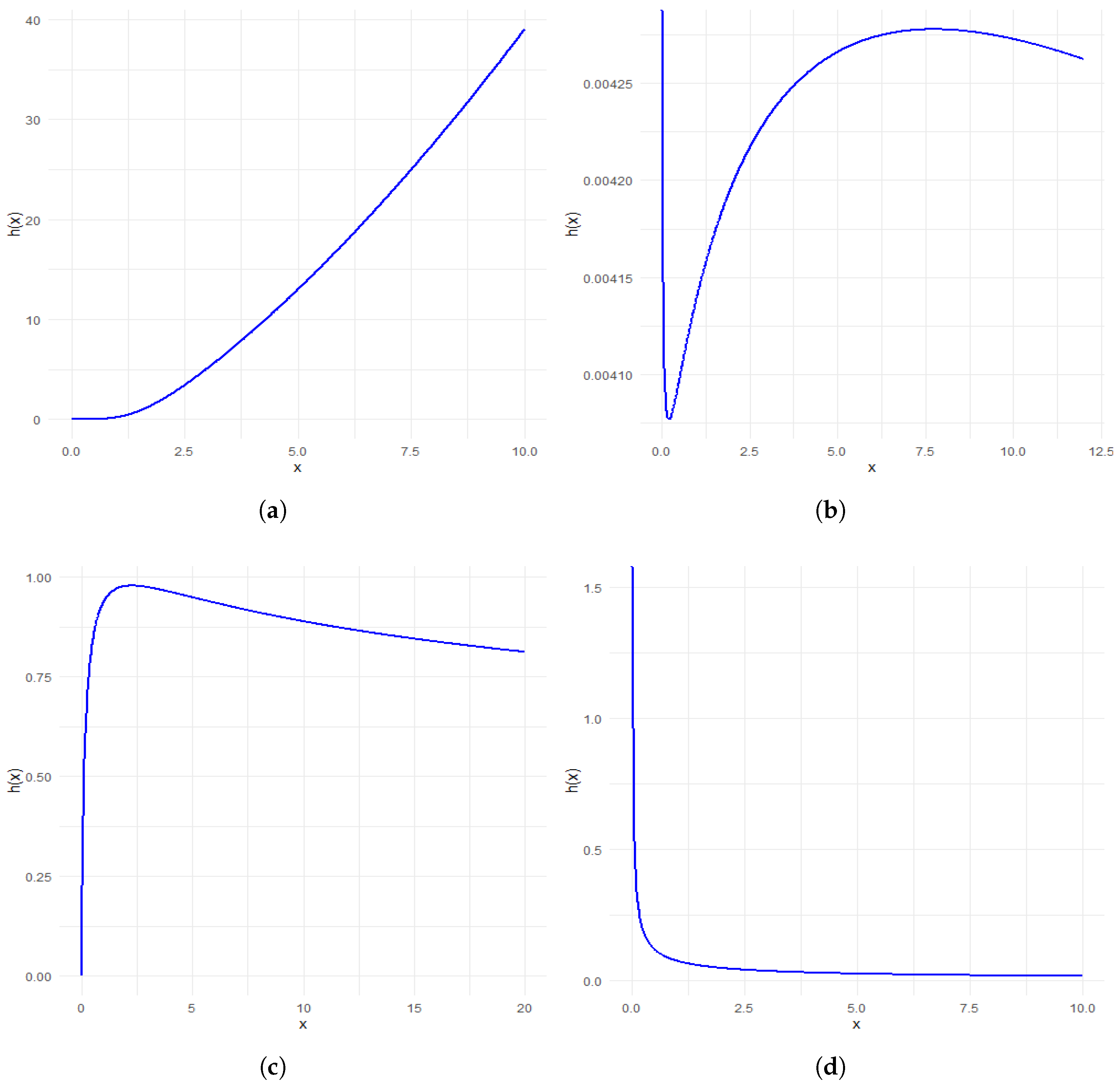

| Parameters () | Number of Change Points of the HRF | Change Points of the HRF |
|---|---|---|
| (0.48, 0.2) | 2 | 0.2038 and 7.7224 |
| (0.8, 2) | 1 | 2.24614 |
| (0.75, 0.1) | 1 | 210.48 |
| (0.45, 0.1) | 2 | 0.9706 and 50.3780 |
| (0.9, 0.5) | 1 | 49.27 |
| n | AE (MLE) | AE (LSE) | MSE (MLE) | MSE (LSE) | ||
|---|---|---|---|---|---|---|
| 0.5 | 0.8 | 20 | 0.5111 | 0.5924 | 0.0026 | 0.7022 |
| 50 | 0.5044 | 0.5020 | 0.0008 | 0.0018 | ||
| 100 | 0.5023 | 0.5011 | 0.0004 | 0.0009 | ||
| 150 | 0.5016 | 0.5007 | 0.0003 | 0.0006 | ||
| 0.6 | 1.0 | 20 | 0.6167 | 0.6227 | 0.0052 | 0.1348 |
| 50 | 0.6066 | 0.6026 | 0.0017 | 0.0041 | ||
| 100 | 0.6033 | 0.6016 | 0.0008 | 0.0019 | ||
| 150 | 0.6023 | 0.6012 | 0.0005 | 0.0012 | ||
| 1.0 | 0.5 | 20 | 1.0150 | 1.0587 | 0.0057 | 0.4178 |
| 50 | 1.0061 | 1.0020 | 0.0020 | 0.0035 | ||
| 100 | 1.0027 | 1.0014 | 0.0010 | 0.0016 | ||
| 150 | 1.0018 | 1.0005 | 0.0006 | 0.0011 | ||
| 2.0 | 1.5 | 20 | 2.0768 | 1.9323 | 0.1027 | 0.1940 |
| 50 | 2.0325 | 1.9758 | 0.0346 | 0.0713 | ||
| 100 | 2.0148 | 1.9882 | 0.0156 | 0.0351 | ||
| 150 | 2.0099 | 1.9938 | 0.0104 | 0.0229 |
| n | AE (MLE) | AE (LSE) | MSE (MLE) | MSE (LSE) | ||
|---|---|---|---|---|---|---|
| 0.5 | 0.8 | 20 | 0.8140 | 0.8075 | 0.0129 | 0.0148 |
| 50 | 0.8067 | 0.8046 | 0.0046 | 0.0054 | ||
| 100 | 0.8032 | 0.8024 | 0.0023 | 0.0027 | ||
| 150 | 0.8024 | 0.8017 | 0.0015 | 0.0018 | ||
| 0.6 | 1.0 | 20 | 1.0187 | 1.0103 | 0.0207 | 0.0237 |
| 50 | 1.0084 | 1.0057 | 0.0075 | 0.0088 | ||
| 100 | 1.0045 | 1.0035 | 0.0037 | 0.0043 | ||
| 150 | 1.0035 | 1.0027 | 0.0024 | 0.0028 | ||
| 1.0 | 0.5 | 20 | 0.5095 | 0.5043 | 0.0046 | 0.0054 |
| 50 | 0.5037 | 0.5022 | 0.0017 | 0.0020 | ||
| 100 | 0.5016 | 0.5015 | 0.0008 | 0.0009 | ||
| 150 | 0.5012 | 0.5007 | 0.0006 | 0.0007 | ||
| 2.0 | 1.5 | 20 | 1.5344 | 1.5174 | 0.0479 | 0.0556 |
| 50 | 1.5121 | 1.5075 | 0.0183 | 0.0208 | ||
| 100 | 1.5071 | 1.5042 | 0.0088 | 0.0102 | ||
| 150 | 1.5047 | 1.5047 | 0.0058 | 0.0068 |
| MODEL | MLEs | K-S | AD | CvM | AIC | BIC |
|---|---|---|---|---|---|---|
| G | (3.9530) | |||||
| (1.6299) | ||||||
| W | (0.3294) | |||||
| (0.0019) | ||||||
| EE | (32.9253) | |||||
| (0.1798) | ||||||
| GL | (23.8138) | |||||
| (0.1850) | ||||||
| PL | (0.3138) | |||||
| (0.0160) | ||||||
| PLXL | (0.3050) | |||||
| (0.0356) |
| MODEL | MLEs | K-S | AD | CvM | AIC | BIC |
|---|---|---|---|---|---|---|
| G | (0.1016) | (0.3127) | (0.3261) | (0.3047) | ||
| (0.0154) | ||||||
| W | (0.0757) | (0.6208) | (0.6209) | (0.5984) | ||
| (0.0638) | ||||||
| EE | (0.1032) | (0.2736) | (0.2797) | (0.2597) | ||
| (0.0157) | ||||||
| GL | (0.0645) | (0.1433) | (0.1151) | (0.1183) | ||
| (0.0196) | ||||||
| PL | (0.0565) | (0.6108) | (0.5859) | (0.5793) | ||
| (0.0920) | ||||||
| PXL | (0.0594) | (0.6286) | (0.5729) | (0.5763) | ||
| (0.0756) | ||||||
| PLXL | (0.0465) | (0.7130) | (0.7711) | (0.7128) | ||
| (0.1367) |
| MODEL | MLEs | AIC | BIC |
|---|---|---|---|
| GIE | (0.0815) | ||
| (0.2691) | |||
| IG | (0.0717) | ||
| (0.2613) | |||
| IW | (0.2091) | ||
| (0.0430) | |||
| IPL | (0.0405) | ||
| (0.2308) | |||
| LN | (0.0958) | ||
| (0.0692) | |||
| LE | (0.0129) | ||
| (0.1606) | |||
| PLXL | (0.0399) | ||
| (0.0596) |
Disclaimer/Publisher’s Note: The statements, opinions and data contained in all publications are solely those of the individual author(s) and contributor(s) and not of MDPI and/or the editor(s). MDPI and/or the editor(s) disclaim responsibility for any injury to people or property resulting from any ideas, methods, instructions or products referred to in the content. |
© 2025 by the authors. Licensee MDPI, Basel, Switzerland. This article is an open access article distributed under the terms and conditions of the Creative Commons Attribution (CC BY) license.
Share and Cite
Kharvi, S.; Irshad, M.R.; Chesneau, C.; Thekkepurayil, J.K.V. Modeling Diverse Hazard Shapes with the Power Length-Biased XLindley Distribution. Math. Comput. Appl. 2026, 31, 4. https://doi.org/10.3390/mca31010004
Kharvi S, Irshad MR, Chesneau C, Thekkepurayil JKV. Modeling Diverse Hazard Shapes with the Power Length-Biased XLindley Distribution. Mathematical and Computational Applications. 2026; 31(1):4. https://doi.org/10.3390/mca31010004
Chicago/Turabian StyleKharvi, Suresha, Muhammed Rasheed Irshad, Christophe Chesneau, and Jabir Kakkottakath Valappil Thekkepurayil. 2026. "Modeling Diverse Hazard Shapes with the Power Length-Biased XLindley Distribution" Mathematical and Computational Applications 31, no. 1: 4. https://doi.org/10.3390/mca31010004
APA StyleKharvi, S., Irshad, M. R., Chesneau, C., & Thekkepurayil, J. K. V. (2026). Modeling Diverse Hazard Shapes with the Power Length-Biased XLindley Distribution. Mathematical and Computational Applications, 31(1), 4. https://doi.org/10.3390/mca31010004


