A Mathematical Framework for E-Commerce Sales Prediction Using Attention-Enhanced BiLSTM and Bayesian Optimization

Abstract

Accurate sales prediction is crucial for inventory and marketing in e-commerce. Cross-border sales involve complex patterns that traditional models cannot capture. To address this, we propose an improved Bidirectional Long Short-Term Memory (BiLSTM) model, enhanced with an attention mechanism and Bayesian hyperparameter optimization. The attention mechanism focuses on key temporal features, improving trend identification. The BiLSTM captures both forward and backward dependencies, offering deeper insights into sales patterns. Bayesian optimization fine-tunes hyperparameters such as learning rate, hidden-layer size, and dropout rate to achieve optimal performance. These innovations together improve forecasting accuracy, making the model more adaptable and efficient for cross-border e-commerce sales. Experimental results show that the model achieves an Root Mean Square Error (RMSE) of 13.2, Mean Absolute Error (MAE) of 10.2, Mean Absolute Percentage Error (MAPE) of 8.7 percent, and a Coefficient of Determination (R²) of 0.92. It outperforms baseline models, including BiLSTM (RMSE 16.5, MAPE 10.9 percent), BiLSTM with Attention (RMSE 15.2, MAPE 10.1 percent), Temporal Convolutional Network (RMSE 15.0, MAPE 9.8 percent), and Transformer for Time Series (RMSE 14.8, MAPE 9.5 percent). These results highlight the model’s superior performance in forecasting cross-border e-commerce sales, making it a valuable tool for inventory management and demand planning.

1. Introduction

Accurate sales forecasting is crucial for e-commerce platforms, especially in cross-border markets where demand exhibits high volatility, pronounced seasonality, and regional heterogeneity [1]. Reliable predictions are essential not only for guiding pricing strategies, marketing planning, and resource allocation [2], but also for improving operational efficiency and anticipating regional consumer behavior [3]. In cross-border e-commerce, precise forecasting helps reduce stockouts and overstocking, enabling better decision-making for global market strategies [4,5]. The complexity of consumer preferences, rapid market fluctuations, and variations in regional demand patterns make forecasting challenging yet critical for sustainable growth and profitability [6].

Traditional time series models like AutoRegressive Integrated Moving Average (ARIMA) and exponential smoothing have long been used to predict sales due to their simplicity and interpretability [7]. However, these models are limited in their ability to capture complex nonlinear patterns and long-term temporal dependencies in dynamic sales data. For example, Gena et al. [8]. applied ARIMA to forecast weekly sales of a footwear brand over three years, effectively capturing sales trends but lacking adaptability to sudden demand fluctuations. Rostan et al. [9] applied ARIMA for option trading strategies during the 2008 financial crisis, achieving successful predictions over a 60-month period. Recently, machine learning methods such as XGBoost have been used for predictive tasks. Wang et al. [10]. utilized XGBoost to model user review-based ratings, extracting valuable consumer behavior features, while Cho et al. [11] compared Long Short-Term Memory (LSTM), Gated Recurrent Unit (GRU), CNN–LSTM, and XGBoost for Water Level prediction. In the financial sector, Tsai et al. [12] highlighted the importance of unified fiscal year-ends for financial comparability, and Khandelwal et al. [13] applied random forests to Amazon EC2 Spot Price prediction, demonstrating superior accuracy compared to linear regression and decision tree models. These studies indicate the effectiveness of modern machine learning models in capturing nonlinear, high-dimensional, and dynamic patterns across diverse domains.

Recent advances in deep learning provide further improvements for sequential data modeling. LSTM networks, introduced by Qin et al. [14], address the vanishing-gradient problem and effectively capture long-term dependencies. BiLSTM, proposed by Su et al. [15], improves prediction accuracy by modeling both forward and backward temporal contexts. Attention mechanisms, first introduced by Bahdanau et al. [16], enable selective focus on critical features, enhancing model interpretability and performance for complex and irregular datasets. Optimal model performance also depends on hyperparameter tuning; traditional grid and random search methods are computationally expensive and may fail to find the best configuration. Bayesian optimization, proposed by Snoek et al. [17], provides an efficient probabilistic framework for tuning hyperparameters and has been successfully applied to various neural network architectures.

Building on recent advances, this study presents an enhanced Attention BiLSTM model, integrated with Bayesian optimization for cross-border e-commerce sales forecasting. The model leverages BiLSTM to capture bidirectional temporal dependencies, incorporates an attention mechanism to selectively emphasize critical features, and employs Bayesian optimization for efficient hyperparameter tuning. Evaluation on real-world e-commerce datasets demonstrates that the proposed approach significantly outperforms traditional LSTM, standard BiLSTM, and ARIMA models in terms of predictive accuracy. Key contributions of this study include the following:

• Architectural Innovation: The design of an enhanced BiLSTM network aims to capture bidirectional temporal dependencies more effectively. It integrates an improved attention mechanism to selectively highlight critical sequential features.
• Attention Mechanism Enhancement: The introduction of a refined attention mechanism that adaptively weighs temporal information, enhancing the focus on influential patterns in complex cross-border e-commerce sales data.
• Hyperparameter Optimization: The application of Bayesian optimization to automatically and efficiently tune key model hyperparameters for optimal performance.
• Empirical Validation of Algorithmic Design: Demonstrate through extensive experiments on a large-scale cross-border e-commerce dataset, that covers multiple product categories, that the proposed structural improvements are effective.

2. Related Work

This section reviews related work on neural networks and attention-based methods for cross-border e-commerce forecasting (Section 2.1 and Section 2.2). By integrating these strands, we identify key gaps addressed by our model, including enhanced bidirectional temporal modeling, adaptive attention, and efficient hyperparameter optimization.

2.1. Neural Networks for Cross-Border E-Commerce

Neural networks have become increasingly important for predicting and analyzing cross-border e-commerce sales because they can model complex, non-linear relationships in data. Unlike traditional statistical methods, neural networks can automatically extract features from large-scale transactional datasets, capturing both temporal patterns and contextual factors such as seasonality, promotions, and regional demand variations [18]. In cross-border settings, where sales are influenced by multiple countries, currencies, and logistics constraints, neural networks provide a flexible framework for integrating heterogeneous data sources and learning meaningful patterns for accurate forecasting.

Moreover, advanced architectures such as LSTM and BiLSTM are particularly effective for handling sequential sales data, as they can retain long-term dependencies and incorporate past trends into future predictions. When combined with attention mechanisms, these models can selectively focus on the most relevant historical sales and external factors, improving interpretability and prediction accuracy [19]. As a result, neural network-based models have become a key tool for decision-making in cross-border e-commerce, enabling companies to optimize inventory, plan marketing strategies, and respond dynamically to global market fluctuations.

2.2. Attention-Based Sales Prediction

Attention-based sales prediction leverages the ability of neural networks to focus on the most relevant parts of historical data when making forecasts [20]. Unlike traditional sequential models that treat all past observations equally, attention mechanisms assign different weights to past time steps, allowing the model to selectively emphasize critical trends, seasonal effects, or promotional events. This approach enhances the model’s interpretability and improves accuracy, especially in complex and volatile sales environments where certain periods or features have disproportionate influence on future demand.

By integrating attention mechanisms with recurrent architectures such as LSTM or BiLSTM, models can capture both long-term dependencies and short-term fluctuations simultaneously. This combination is particularly effective in e-commerce scenarios, where sales patterns are influenced by multiple factors such as consumer behavior, marketing campaigns, and external events [21]. As a result, attention-based models provide a powerful tool for data-driven decision-making, enabling more precise inventory planning, dynamic pricing, and targeted marketing strategies.

3. Fundamentals

This section lays the foundation for our model. We start by reviewing e-commerce sales forecasting methods (Section 3.1). Then, we describe the Bidirectional LSTM structure and mechanism (Section 3.2), introduce Bayesian optimization for hyperparameter tuning (Section 3.3), and explain the enhanced attention mechanism for feature selection (Section 3.4). These concepts provide the technical basis for the methodology in Section 4.

3.1. E-Commerce Sales Forecast

Accurate e-commerce sales forecasting has been addressed using classical statistical and modern machine learning methods. Traditional time series models, such as ARIMA, model a univariate sales series $\left\{y_t\right\}$ as follows:

$$\mathrm{\Phi }\left(L\right){(1-L)}^d{y}_t=\mathrm{\Theta }\left(L\right){ϵ}_t+\sum _{j=1}^p{\alpha }_j{y}_{t-j}+\sum _{k=1}^q{\beta }_k{ϵ}_{t-k},{ϵ}_t\sim \mathcal{N}(0,{\sigma }^2),$$

(1)

where L is the lag operator, d the differencing order, $\mathrm{\Phi }\left(L\right)$ and $\mathrm{\Theta }\left(L\right)$ are AR and MA polynomials, and ${\alpha }_j,{\beta }_k$ denote additional lag coefficients capturing complex autocorrelations.The parameters p and q are the orders of the autoregressive (AR) and moving average (MA) components, respectively. The coefficients ${\alpha }_j$ and ${\beta }_k$ capture the influence of past sales and noise terms. The time series $y_t$ represents univariate sales, and the error terms ${ϵ}_t$ follow a normal distribution, $\mathcal{N}(0,{\sigma }^2)$, with dimensions $1\times 1$. This formulation allows modeling higher-order dependencies and enhanced seasonal structures.

Gradient boosting, particularly XGBoost, has shown strong performance in handling nonlinear, high-dimensional features. Given input features $X=[x_1,\dots ,x_n]$ (where each $x_i$ is a vector of features for the i-th sample) and target y, XGBoost constructs an additive model with interaction depth d:

$${\widehat{y}}_i=\sum _{k=1}^K{f}_k\left(x_i\right)=\sum _{k=1}^K\sum _{j=1}^d{w}_{kj}\mathbb{I}(x_i\in R_{kj}),f_k\in \mathcal{F},$$

(2)

where $f_k\left(x_i\right)$ is the contribution of the k-th base function, $w_{kj}$ is the weight of the j-th split, and $\mathbb{I}(x_i\in R_{kj})$ is an indicator function that is 1 if $x_i$ is in region $R_{kj}$, and 0 otherwise. The model is built by iteratively adding functions from the function space $\mathcal{F}$ to minimize residuals.The model is constructed by iteratively adding functions from the function space $\mathcal{F}$ to minimize the following regularized objective function:

$$\mathcal{L}=\sum _{i=1}^{N}l\left(y_i,\sum _{k=1}^K{f}_k\left(x_i\right)\right)+\sum _{k=1}^K\left(\gamma T_k+{\displaystyle \frac{1}{2}}\lambda \sum _{j=1}^{T_k}{w}_{kj}^2\right),$$

(3)

where $R_{kj}$ represents the j-th leaf region of the k-th tree, $T_k$ the number of leaves, and $w_{kj}$ the corresponding leaf weight. This formulation captures nonlinear interactions and hierarchical feature effects.

3.2. Bidirectional LSTM

BiLSTM networks are designed to capture both past and future dependencies in sequence data [22], making them particularly suitable for time series with volatile and asymmetric patterns, such as cross-border e-commerce sales. This characteristic also makes BiLSTM more suitable than Transformer models for small datasets, where attention-based Transformers may overfit or be sensitive to noise.

For an input sequence $X=\{x_1,x_2,\dots ,x_T\}$, the bidirectional hidden states are computed as follows:

$$H=\overrightarrow{H}\oplus \overleftarrow{H}=\sigma \left(X{W}_f+{\overrightarrow{H}}_{-1}{U}_f+X{W}_b+{\overleftarrow{H}}_{+1}{U}_b+B\right)$$

(4)

where X is the input sequence of size $T\times d$, $\overrightarrow{H}$ and $\overleftarrow{H}$ are the forward and backward hidden states with dimensions $T\times h$, $W_f$ and $W_b$ are weight matrices of size $d\times h$ and $h\times h$ respectively, $U_f$ and $U_b$ are weight matrices for the previous hidden state of size $h\times h$, and B is the bias vector of size h. The operator ⊕ denotes the concatenation of the forward and backward hidden states. This bidirectional structure enables the model to consider both historical and future information at each time step, which is especially effective in capturing temporal dynamics in short and volatile sequences, where global attention alone may be less reliable.

To aggregate the sequence information into a single context vector and emphasize the most relevant time steps, we apply a multi-head attention mechanism:

$$\widehat{H}=\sum _{t=1}^T\sum _{m=1}^M{\displaystyle \frac{exp\left({\mathbf{v}}_m^{\top }tanh(W_{\alpha }^m{h}_t+b_{\alpha }^m)\right)}{{\sum }_{k=1}^{T}exp\left({\mathbf{v}}_m^{\top }tanh(W_{\alpha }^m{h}_k+b_{\alpha }^m)\right)}}{h}_t$$

(5)

Here, $h_t$ is the concatenated hidden state, $W_{\alpha }^m$ and $b_{\alpha }^m$ are the attention weight matrices and biases for head m, and ${\mathbf{v}}_m$ is the attention vector. This mechanism allows the model to dynamically assign higher importance to critical time steps, such as sudden demand spikes or seasonal peaks. Compared with Transformer-based models, this selective focus enables BiLSTM to better handle short sequences and volatile data while avoiding overfitting.

Finally, the prediction and training objective are defined as follows:

$$\widehat{y}=\varphi (\widehat{H}{W}_y+b_y),\mathcal{L}\left(\theta \right)={\displaystyle \frac{1}{N}}\sum _{i=1}^N\parallel {\widehat{y}}_i-y_i{\parallel }^2+\lambda {\parallel \theta \parallel }^2$$

(6)

where $\widehat{y}$ is the predicted output, $W_y$ is the output weight matrix, $b_y$ is the bias, $\varphi$ is the activation function, and $\lambda$ controls regularization to prevent overfitting. By combining BiLSTM with attention, the model efficiently captures temporal dependencies and highlights key time steps, making it more robust than Transformers for small, highly volatile datasets. This justifies our choice of BiLSTM for the current study.

3.3. Hyperparameter Optimization in Deep Learning Models

Hyperparameter optimization is critical for improving deep learning models, particularly in high-dimensional search spaces. Bayesian optimization has proven effective by using a probabilistic surrogate model to estimate the objective function $f\left(\theta \right)$ and guide the search for optimal hyperparameters ${\theta }^{\ast }$. The goal is to maximize the objective:

$${\theta }^{\ast }=arg\underset{\theta }{max}\mathbb{E}\left[f\left(\theta \right)\right],$$

(7)

where $\mathbb{E}\left[f\right(\theta \left)\right]$ denotes the expected value of the objective function. To model $f\left(\theta \right)$, a Gaussian Process (GP) posterior is used, given by the following:

$$p\left(f\left(\theta \right)\right|D)=\mathcal{N}(f\left(\theta \right);\mu \left(\theta \right),\Sigma (\theta ,{\theta }^{\prime })),$$

(8)

where $\mu \left(\theta \right)$ is the mean prediction and $\mathrm{\Sigma }(\theta ,{\theta }^{\prime })$ is the covariance function. The acquisition function, such as Expected Improvement (EI), guides the search by evaluating the expected improvement over the current best solution:

$$\mathrm{EI}\left(\theta \right)=(f_{\mathrm{best}}-\mu \left(\theta \right))\mathrm{\Phi }\left({\displaystyle \frac{f_{\mathrm{best}}-\mu \left(\theta \right)}{\sigma \left(\theta \right)}}\right)+\sigma \left(\theta \right)\varphi \left({\displaystyle \frac{f_{\mathrm{best}}-\mu \left(\theta \right)}{\sigma \left(\theta \right)}}\right),$$

(9)

where $f_{\mathrm{best}}$ is the current best value, and $\mu \left(\theta \right)$ and $\sigma \left(\theta \right)$ are the predicted mean and standard deviation. The dimensions of $\mu \left(\theta \right)$ and $\sigma \left(\theta \right)$ are both $1\times 1$.

3.4. Attention Mechanism Enhancement for Sequential Feature Highlighting

Attention mechanisms enable models to focus on relevant parts of an input sequence. For a sequence of length T and feature dimension d, scaled dot-product attention with multiple heads and masking can be expressed as follows:

$${\mathbf{A}}_{t,i}^{\left(h\right)}={\displaystyle \frac{exp\left(\left({\mathbf{Q}}_t^{\left(h\right)}{\mathbf{K}}_i^{\left(h\right)\top }\right)/\sqrt{d_k}+M_{t,i}^{\left(h\right)}\right)}{{\sum }_{j=1}^{T}exp\left(\left({\mathbf{Q}}_t^{\left(h\right)}{\mathbf{K}}_j^{\left(h\right)\top }\right)/\sqrt{d_k}+M_{t,j}^{\left(h\right)}\right)}},t,i=1,\dots ,T,h=1,\dots ,H,$$

(10)

where ${\mathbf{Q}}^{\left(h\right)},{\mathbf{K}}^{\left(h\right)},{\mathbf{V}}^{\left(h\right)}\in {\mathbb{R}}^{T\times d_k}$ are the queries, keys, and values for head h, and $M^{\left(h\right)}\in {\mathbb{R}}^{T\times T}$ is an optional mask.

The context tensors for each head are computed as follows:

$${\widehat{\mathbf{H}}}_t^{\left(h\right)}=\sum _{i=1}^T{\mathbf{A}}_{t,i}^{\left(h\right)}{\mathbf{V}}_i^{\left(h\right)}\in {\mathbb{R}}^{d_k},t=1,\dots ,T,h=1,\dots ,H.$$

(11)

For full batch processing, multi-head attention can be written as a 4D tensor operation:

$${\mathbf{Z}}_{b,t,h,k}=\sum _{i=1}^T{\displaystyle \frac{exp\left(({\mathbf{Q}}_{b,t,h,:}·{\mathbf{K}}_{b,i,h,:}^{\top })/\sqrt{d_k}+M_{b,t,i,h}\right)}{{\sum }_{j=1}^{T}exp\left(({\mathbf{Q}}_{b,t,h,:}·{\mathbf{K}}_{b,j,h,:}^{\top })/\sqrt{d_k}+M_{b,t,j,h}\right)}}{\mathbf{V}}_{b,i,h,k},$$

(12)

$${\mathrm{Output}}_{b,t,:}={\mathrm{Concat}}_{h=1}^H{\mathbf{Z}}_{b,t,h,:}{W}_h^O+b^O,b=1,\dots ,B,t=1,\dots ,T,k=1,\dots ,d_k,$$

(13)

where B is the batch size and $W^O\in {\mathbb{R}}^{H{d}_k\times d}$. ${\mathbf{Q}}_{b,t,h,:}$, ${\mathbf{K}}_{b,i,h,:}$, and ${\mathbf{V}}_{b,i,h,k}$ are the query, key, and value matrices for the b-th batch, t-th timestep, h-th attention head, and i-th timestep. The dimensions of $\mathbf{Q}$, $\mathbf{K}$, and $\mathbf{V}$ are $(B,T,H,D)$, and $M_{b,t,i,h}$ is a masking term with dimensions $(B,T,T,H)$.

4. Methodology

This section presents our Enhanced BiLSTM model for cross-border e-commerce sales forecasting. We describe the core architecture (Section 4.1), adaptive attention mechanism (Section 4.2), Bayesian optimization for hyperparameter tuning (Section 4.3), and the full method overview (Section 4.4). Each component addresses model limitations, ensuring better accuracy and robustness.

4.1. Enhanced BiLSTM Network with Attention and Residual Connections

In time series forecasting, traditional LSTMs capture long-range dependencies but are limited by their unidirectional structure. BiLSTMs address this by processing sequences in both directions, yet they still struggle to prioritize the most relevant time steps, particularly in complex tasks like cross-border e-commerce sales forecasting. To overcome these challenges, we propose an Enhanced BiLSTM Network with dual-activation attention and residual connections, which selectively focuses on important time steps while preserving long-term dependencies, making it more suitable than Transformer-based models for small, volatile datasets.

Given an input sequence $X=\{x_1,x_2,\dots ,x_T\}$, the BiLSTM generates bidirectional hidden states $H=\{h_1,h_2,\dots ,h_T\}$, where $h_t=[\overrightarrow{h_t};\overleftarrow{h_t}]$ is the concatenation of forward and backward states at each time step. This bidirectional structure allows the model to capture both past and future dependencies, which is crucial for modeling asymmetric temporal effects in volatile sales data.

To focus on the most relevant time steps, we introduce an advanced attention mechanism that applies non-linear transformations and multiplicative interactions. The attention weight ${\alpha }_t$ is calculated as follows:

$${\alpha }_t={\displaystyle \frac{exp\left({\mathbf{v}}^{\top }·\mathrm{ReLU}({\mathbf{W}}_a{h}_t+{\mathbf{b}}_a)+{\mathbf{c}}^{\top }·\mathrm{sigmoid}({\mathbf{W}}_a^{\left(2\right)}{h}_t+{\mathbf{b}}_a^{\left(2\right)})\right)}{{\sum }_{k=1}^{T}exp\left({\mathbf{v}}^{\top }·\mathrm{ReLU}({\mathbf{W}}_a{h}_k+{\mathbf{b}}_a)+{\mathbf{c}}^{\top }·\mathrm{sigmoid}({\mathbf{W}}_a^{\left(2\right)}{h}_k+{\mathbf{b}}_a^{\left(2\right)})\right)}},$$

(14)

where ReLU emphasizes significant temporal features, such as seasonal peaks or promotions, while sigmoid attenuates less relevant signals, allowing the model to balance sensitivity to short-term fluctuations with the preservation of long-term trends. This dual-activation attention is particularly effective for small, volatile datasets where global attention mechanisms of Transformers may overfit or be sensitive to noise. The weighted hidden state is then computed as follows:

$${\widehat{h}}_t={\alpha }_t·\left({\mathbf{W}}_h·\mathrm{LeakyReLU}\left({\mathbf{W}}_h^{\left(2\right)}{h}_t+{\mathbf{b}}_h^{\left(2\right)}\right)\right),$$

(15)

where LeakyReLU allows gradients to propagate for negative activations, avoiding dead neurons and improving learning of low-activation features. This further enhances robustness in volatile sequences.

To enhance the model further, we incorporate residual connections. The residual-modified state $h_t^{\mathrm{res}}$ is defined as follows:

$$h_t^{\mathrm{res}}=\left(h_t+\gamma ·\tan \mathrm{h}\left({\mathbf{W}}_r·\mathrm{ReLU}\left({\mathbf{W}}_r^{\left(2\right)}{h}_t+{\mathbf{b}}_r^{\left(2\right)}\right)\right)\right)·\mathrm{sigmoid}\left({\mathbf{W}}_r^{\left(3\right)}{h}_t+{\mathbf{b}}_r^{\left(3\right)}\right),$$

(16)

where the residual connections help prevent vanishing gradients and combine transformed features with original hidden states, improving the model’s ability to capture complex temporal dependencies.The final prediction ${\widehat{y}}_t$ is computed as follows:

$${\widehat{y}}_t={\mathbf{W}}_y·\left(h_t^{\mathrm{res}}\right)·\mathrm{softmax}\left({\mathbf{W}}_y^{\left(2\right)}·h_t^{\mathrm{res}}+{\mathbf{b}}_y^{\left(2\right)}\right)+{\mathbf{b}}_y,$$

(17)

where the softmax normalization and linear projections map the enhanced hidden states to the output space, making the model capable of forecasting both normal and extreme fluctuations. Overall, this Enhanced BiLSTM framework is well-suited to small, highly volatile cross-border e-commerce sales data, offering greater stability and generalization than Transformer-based approaches on the current dataset.

The pseudocode for the methodology is summarized in Algorithm 1, highlighting the encoding, dual-activation attention, residual enhancement, and output projection steps.

Algorithm 1 Enhanced BiLSTM with Dual-Activation Attention and Residual Connections

Input: Time series $X\in {\mathbb{R}}^{T\times d}$  Output: Predicted values $\widehat{Y}\in {\mathbb{R}}^{T\times d_y}$     1.  BiLSTM Encoding: $h_t=[\overrightarrow{h_t};\overleftarrow{h_t}],H=\{h_1,\dots ,h_T\}$     2.  Dual-Activation Attention: $e_t={\mathbf{v}}^{\top }\mathrm{ReLU}({\mathbf{W}}_a{h}_t+{\mathbf{b}}_a)+{\mathbf{c}}^{\top }\mathrm{sigmoid}({\mathbf{W}}_a^{\left(2\right)}{h}_t+{\mathbf{b}}_a^{\left(2\right)})$ ${\alpha }_t=\mathrm{softmax}\left(e_t\right)$     3.  Weighted Hidden Representation: ${\widehat{h}}_t={\alpha }_t·[{\mathbf{W}}_h·\mathrm{LeakyReLU}({\mathbf{W}}_h^{\left(2\right)}{h}_t+{\mathbf{b}}_h^{\left(2\right)})]$     4.  Residual Enhancement: $r_t=tanh({\mathbf{W}}_r·\mathrm{ReLU}({\mathbf{W}}_r^{\left(2\right)}{h}_t+{\mathbf{b}}_r^{\left(2\right)}))$ $g_t=\mathrm{sigmoid}({\mathbf{W}}_r^{\left(3\right)}{h}_t+{\mathbf{b}}_r^{\left(3\right)})$ $h_t^{\mathrm{res}}=(h_t+\gamma ·r_t)\odot g_t$     5.  Output Projection: ${\widehat{y}}_t={\mathbf{W}}_y·h_t^{\mathrm{res}}·\mathrm{softmax}({\mathbf{W}}_y^{\left(2\right)}{h}_t^{\mathrm{res}}+{\mathbf{b}}_y^{\left(2\right)})+{\mathbf{b}}_y$     6.  Return: $\widehat{Y}=\{{\widehat{y}}_1,{\widehat{y}}_2,\dots ,{\widehat{y}}_T\}$

4.2. Adaptive Attention Mechanism

In cross-border e-commerce sales forecasting, time-series data often exhibit complex patterns, including seasonality, promotions, and sudden spikes. Moreover, the data is often limited in length, with high volatility, making it challenging for models to focus on the most relevant time steps. To address this, we propose an adaptive attention mechanism that dynamically assigns importance to each time step, guided by both current and historical hidden states. Let $h_t$ denote the hidden state at time step t. We first apply dual non-linear transformations:

$$u_t=tanh({\mathbf{W}}_u{h}_t+{\mathbf{b}}_u)\odot \mathrm{sigmoid}({\mathbf{W}}_s{h}_t+{\mathbf{b}}_s)$$

(18)

where the combination of tanh and sigmoid allows the model to simultaneously capture strong and subtle patterns. tanh emphasizes the dominant temporal signals, such as promotional peaks, while sigmoid acting as a gating mechanism to downweight noisy or less informative time steps. This design aligns with the dual-mode demand dynamics observed in cross-border e-commerce data. Next, we incorporate temporal context interaction by considering the previous hidden state:

$${\tilde{e}}_t={\mathbf{v}}^{\top }{u}_t+\gamma ·\left({\mathbf{h}}_{t-1}^{\top }{\mathbf{W}}_c{h}_t\right)$$

(19)

The term ${\mathbf{h}}_{t-1}^{\top }{\mathbf{W}}_c{h}_t$ captures dependencies between consecutive time steps, which is critical for short, volatile sequences where past sales patterns influence current demand. The learnable scaling factor $\gamma$ adjusts the relative contribution of historical context. The attention weight for each time step is then obtained using a softmax function:

$${\alpha }_t={\displaystyle \frac{exp\left({\tilde{e}}_t\right)}{{\sum }_{k=1}^{T}exp\left({\tilde{e}}_k\right)}}$$

(20)

This normalization ensures that the model selectively focuses on key time steps, giving higher weight to critical events such as promotions, seasonal peaks, or sudden demand spikes, while suppressing irrelevant fluctuations. Finally, the weighted hidden state is computed as follows:

$${\widehat{h}}_t={\alpha }_t·({\mathbf{W}}_h{h}_t+{\mathbf{b}}_h)$$

(21)

where ${\widehat{h}}_t$ is the resulting context-aware representation. This adaptive weighting is particularly effective for small, volatile datasets, allowing the BiLSTM to prioritize informative temporal features without overfitting.

4.3. Hyperparameter Optimization

Model performance is highly sensitive to hyperparameters, especially in small or noisy datasets. To ensure robust and stable forecasting, we adopt Bayesian optimization for systematic hyperparameter tuning. This approach balances exploration of the hyperparameter space with exploitation of promising configurations, which is crucial when the dataset is limited in size.

Let $\theta$ denote the set of hyperparameters, such as learning rate, hidden layer size, dropout rate, and attention layer weight initialization. The objective is to find the optimal ${\theta }^{\ast }$ that minimizes a validation loss function ${\mathcal{L}}_{val}\left(\theta \right)$ within a feasible search space $\mathrm{\Theta }$:

$${\theta }^{\ast }=arg\underset{\theta \in \mathrm{\Theta },{\theta }_{min}\le \theta \le {\theta }_{max}}{min}{\mathcal{L}}_{val}\left(\theta \right),$$

(22)

where ${\theta }_{min}$ and ${\theta }_{max}$ define practical bounds for each hyperparameter.

Bayesian optimization approximates the unknown objective function ${\mathcal{L}}_{val}\left(\theta \right)$ using a probabilistic surrogate, typically a Gaussian Process (GP) with observation noise:

$${\mathcal{L}}_{val}\left(\theta \right)\sim \mathcal{GP}\left(\mu \left(\theta \right),k(\theta ,{\theta }^{\prime })+{\sigma }_n^2{\delta }_{\theta ,{\theta }^{\prime }}\right),$$

(23)

where $\mu \left(\theta \right)$ is the mean function, $k(\theta ,{\theta }^{\prime })$ is the covariance kernel, ${\sigma }_n^2$ represents observation noise, and ${\delta }_{\theta ,{\theta }^{\prime }}$ is the Kronecker delta function.

By using the GP surrogate, Bayesian optimization efficiently predicts promising hyperparameters even with limited evaluations, which is particularly useful for small cross-border sales datasets that cannot support exhaustive grid search.

To select the next hyperparameter configuration, an acquisition function is used. We adopt the Expected Improvement (EI) criterion, which balances exploration and exploitation:

$$\mathrm{EI}\left(\theta \right)=\mathbb{E}\left[max(0,{\mathcal{L}}_{val}^{best}-{\mathcal{L}}_{val}\left(\theta \right))\right]=({\mathcal{L}}_{val}^{best}-{\mu }_t\left(\theta \right))\mathrm{\Phi }\left(Z\right)+{\sigma }_t\left(\theta \right)\varphi \left(Z\right),$$

(24)

$$Z={\displaystyle \frac{{\mathcal{L}}_{val}^{best}-{\mu }_t\left(\theta \right)}{{\sigma }_t\left(\theta \right)}},$$

(25)

where ${\mu }_t\left(\theta \right)$ and ${\sigma }_t^2\left(\theta \right)$ are the predictive mean and variance from the GP at iteration t; ${\mathcal{L}}_{val}^{best}$ is the best observed loss; and $\mathrm{\Phi }$ and $\varphi$ denote the standard normal CDF and PDF.

The next hyperparameter candidate is then chosen as follows:

$${\theta }_{t+1}=arg\underset{\theta \in \mathrm{\Theta }}{max}\mathrm{EI}(\theta \mid {\mathcal{D}}_t),$$

(26)

where ${\mathcal{D}}_t={\left\{({\theta }_i,{\mathcal{L}}_{val}\left({\theta }_i\right))\right\}}_{i=1}^t$ represents the set of hyperparameters evaluated up to iteration t.

Through iterative updates, Bayesian optimization efficiently converges to the optimal configuration ${\theta }^{\ast }$, improving model generalization and stability across different product categories and time periods. This is especially important for small, volatile cross-border e-commerce datasets, where manual tuning or naive search strategies may fail to achieve consistent performance.

4.4. Overview of the Proposed Method

Traditional time series models often fail to capture the complex, nonlinear, and seasonal patterns in international e-commerce sales data. Additionally, Transformer-based models can struggle with small datasets and highly volatile sequences due to their large parameter count and sensitivity to noise. To address these challenges, we propose an enhanced BiLSTM model with a dual-activation attention mechanism and Bayesian hyperparameter optimization, which balances expressiveness and robustness for limited, irregular sales data.

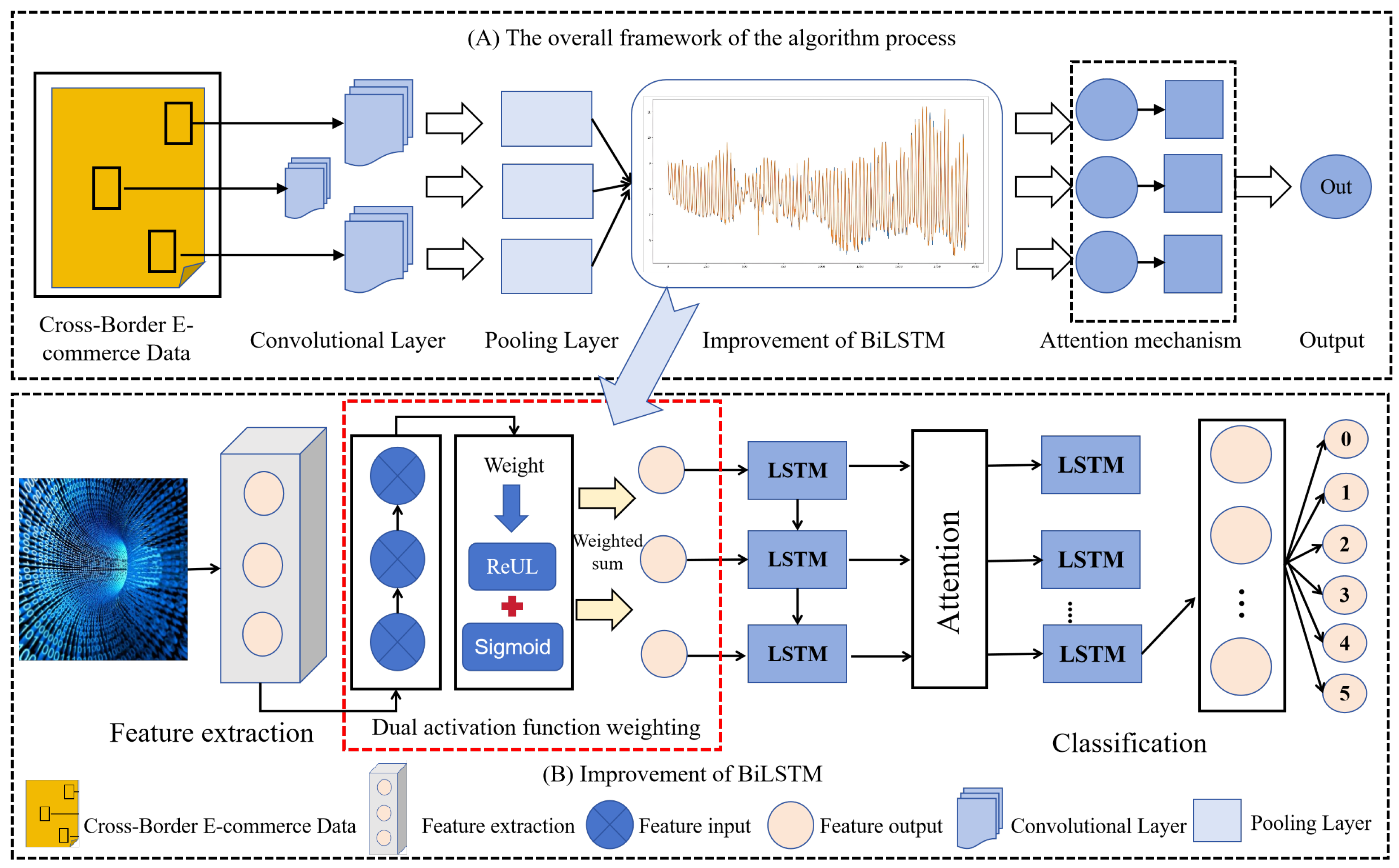
The framework consists of four core modules. The BiLSTM captures bidirectional dependencies, leveraging both past and future information. Its recurrent structure efficiently models temporal patterns in short sequences, mitigating overfitting compared to Transformers. The attention mechanism dynamically assigns weights to key time steps and features, emphasizing patterns such as seasonal trends, promotions, and sudden sales spikes. The dual-activation mechanism (ReLU + Sigmoid) further allows the model to amplify strong signals while suppressing noise, providing selective temporal feature weighting aligned with the irregular nature of cross-border sales. Bayesian optimization automatically tunes critical hyperparameters, including learning rate, hidden layer size, and dropout rate, ensuring optimal performance without manual tuning. This automated tuning is particularly important for volatile datasets, where sensitivity to hyperparameters can significantly impact forecasting stability.

Figure 1 illustrates the overall architecture. Input sales sequences are processed by BiLSTM layers to obtain hidden states, which are then weighted by the adaptive attention module. The resulting sequence representation is passed to the output layer for sales prediction, with hyperparameters optimized via Bayesian optimization to enhance generalization and stability across diverse e-commerce datasets. This design ensures that both strong seasonal/promotional patterns and subtle, context-dependent trends are captured effectively.

As shown in Figure 1, the model follows a clear and theoretically justified flow to capture complex sales patterns:

• BiLSTM Input Processing: The input time series is processed by the BiLSTM layer, which captures both past trends and future events, such as upcoming promotions. Its bidirectional modeling is especially effective for short, volatile sequences where long-range attention may be less reliable.
• Dual-Activation Module: A dual-activation mechanism applies both ReLU and Sigmoid to the BiLSTM hidden states. ReLU amplifies strong, discriminative signals (e.g., promotional spikes), while Sigmoid attenuates weak or noisy signals (e.g., regular months without promotions). This complementary design enables selective feature amplification and gating, improving the model’s ability to capture both short-term fluctuations and long-term trends.
• Adaptive Attention Mechanism: The attention module dynamically adjusts the weight of each time step. During peak seasons, like Black Friday, it assigns higher importance to promotional periods while reducing the influence of irrelevant data. Combined with dual-activation preprocessing, this mechanism ensures that the model focuses on both strong events and contextually relevant patterns.
• Residual Connections: Residual connections are added between the BiLSTM and attention layers. These connections stabilize training by preserving key features, preventing gradient vanishing, and enabling more complex interactions between original and transformed hidden states.
• Bayesian Optimization: Bayesian optimization tunes hyperparameters such as learning rate, hidden layer size, and dropout rate automatically. This adaptive tuning improves model generalization and stability, particularly important for small datasets with high volatility, where manual tuning may fail to achieve consistent performance.

Together, these components provide a principled and effective forecasting framework: the BiLSTM efficiently captures bidirectional temporal dependencies, the dual-activation attention module selectively emphasizes relevant time steps, residual connections enhance feature propagation, and Bayesian optimization ensures stable and optimal hyperparameter settings. This integrated design is particularly suitable for small, volatile cross-border e-commerce datasets, where Transformers may struggle with overfitting or noise sensitivity.

5. Experimental Setup

This section outlines the experimental design. We cover data and preprocessing (Section 5.1 and Section 5.2), experimental setup and training parameters (Section 5.3), baseline algorithms (Section 5.4), and evaluation metrics (Section 5.5). This ensures reliable results for assessing the model’s performance in cross-border e-commerce sales forecasting.

5.1. Data Source

The dataset used in this study is collected from the Amazon e-commerce platform, which is one of the largest and most diverse international online marketplaces (Amazon Sales Dataset: https://www.kaggle.com/datasets/karkavelrajaj/amazon-sales-dataset, accessed on 15 June 2025). The data encompasses historical sales records across multiple product categories, including electronics, home appliances, clothing, and personal care items. Each record contains time-stamped information such as sales volume, product identifier, category, price, discount, and relevant promotional events [23].

To ensure data quality and relevance for cross-border e-commerce sales forecasting, we handled missing values, detected outliers and normalized the data. Seasonal patterns, promotional spikes, and other irregular events were preserved to capture the inherent complexity of the sales dynamics on the Amazon platform. The resulting dataset provides a rich and high-resolution time series suitable for training and evaluating the proposed Enhanced BiLSTM model with adaptive attention and Bayesian hyperparameter optimization.

5.2. Data Preprocessing

The dataset used in this study is collected from the Amazon e-commerce platform Amazon Sales Dataset. In real-world data, noise, missing values, and inconsistencies may adversely affect model performance. Therefore, a systematic preprocessing procedure is applied before feature selection and model training. The main steps are as follows. An example of the processed dataset is shown in

Table 1. Preprocessed monthly sales data for Amazon products.

Month	Year	Product Category	Units Sold	Promotion	Season (Quarter)
1	2022	Electronics	1200	0	1
2	2022	Electronics	1350	0	1
3	2022	Electronics	1420	1	1
4	2022	Electronics	1300	0	2
5	2022	Home Appliances	950	0	2
6	2022	Home Appliances	870	1	2
7	2022	Clothing	2100	0	3
8	2022	Clothing	2350	1	3
9	2022	Personal Care	1500	0	3
10	2022	Personal Care	1650	1	4
11	2022	Electronics	1400	1	4
12	2022	Electronics	1550	1	4
13	2023	Electronics	1600	0	1
14	2023	Home Appliances	980	0	1
15	2023	Clothing	2400	1	1

.

• Data Cleaning: Duplicate records and missing entries are removed to ensure data quality. Outliers, such as extremely high or low sales values caused by data entry errors or exceptional events, are detected and handled appropriately. This step ensures that the data fed into the model is reliable and consistent.
• Data Encoding: Time-related features are extracted from the original timestamps, which are at a daily granularity. Numeric fields for year and month are created, e.g., year values as 2022, 2023, and month values as 1–12, to enable temporal modeling at monthly granularity.
• Data Aggregation: Sales are aggregated at the monthly level, which is an important granularity for capturing seasonal patterns and promotional effects. Analysis of historical sales shows that demand varies significantly across months, with peaks during promotional seasons such as Prime Day or Black Friday.
• Feature Construction: To capture seasonal effects, a numeric seasonal feature is added representing the quarter (1 to 4). Promotional activity is encoded as a binary feature, with 1 indicating the presence of a sale or discount campaign during the month and 0 otherwise. Additionally, other relevant product attributes, such as category, price tier, and rating, are included as features to enhance model performance.

After these preprocessing steps, the resulting dataset provides a clean, aggregated, and feature-rich time series of monthly sales for multiple product categories on the Amazon platform. This dataset is suitable for training and evaluating the proposed Enhanced BiLSTM model with adaptive attention and Bayesian hyperparameter optimization.

5.3. Experimental Environment and Parameter Settings

All experiments were conducted in a Python-based environment managed with Anaconda, using Python 3.8 as the development IDE. This setup ensures reproducible and efficient training for the proposed forecasting model. The detailed environment configuration and key parameter settings for the proposed model and all baseline algorithms are summarized in

Table 2. Experimental environment configuration.

Component	Specification
Python Version	3.10
Platform	Anaconda 3
Development IDE	PyCharm 2025.3
Hardware	Intel Core i7, 16 GB RAM, NVIDIA RTX 3060
Dataset Split	Training: Testing = 7:3 (time-based split)
	First 16 months for training, last 8 months for testing
General Training Parameters	Batch size = 64, Epochs = 300
Hyperparameter Search Ranges	Dropout rate: 0.1–0.5
	Learning rate: 0.0001–0.01

and

Table 3. Hyperparameter values for all models.

Model	Learning Rate	Hidden Units	Attention Dim.	Dropout Rate	Other Key Parameters
ARIMA	–	–	–	–	Seasonal period = 12
Standard LSTM	0.001	128	–	0.2	Layers = 2
BiLSTM	0.001	128	–	0.2	Layers = 2
BiLSTM + Attention	0.001	128	64	0.2	Layers = 2, Attention heads = 1
TCN	0.001	64	–	0.2	Layers = 4, Kernel size = 3, Dilation = 2
TFT	0.001	128	64	0.2	Encoder layers = 2, Attention heads = 2
Proposed Enhanced BiLSTM	0.001	128	64	0.2	Layers = 2, Residual $\gamma$ = 0.1, Dual-attention

.

5.3.1. Experimental Environment Configuration

This subsection describes the experimental environment and general training configuration used for all models to ensure reproducibility and fair comparison. All experiments were conducted in a unified software and hardware environment, and identical data preprocessing and training protocols were applied across the proposed model and all baseline algorithms. The detailed environment configuration, including software versions, hardware specifications, dataset split strategy, and general training parameters, is summarized in Table 2.

To account for the stochastic nature of deep learning training, each neural network model was executed 10 times with different random seeds under the same environment configuration shown in Table 2. The reported experimental results correspond to the mean performance across these runs, with standard deviations provided where applicable. This repeated-experiment protocol enhances the robustness of the results and provides a reliable basis for subsequent statistical significance analysis.

5.3.2. Model-Specific Parameter Settings

This subsection details the model-specific hyperparameter configurations used in the experiments. To ensure a fair and unbiased comparison, all baseline models were tuned using grid search with 3-fold time-based cross-validation on the training set, while the proposed Enhanced BiLSTM model was optimized using Bayesian optimization, as described in Section 4.3. The hyperparameter search ranges were kept consistent across models whenever applicable, and the best-performing configuration for each model was selected based on validation RMSE. The final selected hyperparameter values for all models are summarized in Table 3.

As shown in Table 3, the adopted parameter configuration strategy ensures experimental consistency and optimization fairness across all compared models. By sharing core training settings and comparable hyperparameter search spaces, performance differences can be attributed primarily to architectural design rather than experimental bias. Furthermore, several parameters were tailored to the characteristics of cross-border e-commerce sales data, such as the seasonal period of 12 for ARIMA to capture annual monthly seasonality, and the residual weighting factor $\gamma =0.1$ in the proposed model to balance feature propagation and training stability.

5.4. Comparison Algorithms

To evaluate the performance of the proposed Enhanced BiLSTM model with adaptive attention and Bayesian hyperparameter optimization, six baseline algorithms are considered. First, ARIMA, a classical statistical model, is included to capture linear and seasonal dependencies in time series data. Standard LSTM [24], a unidirectional LSTM network, and BiLSTM, a bidirectional LSTM [25] that leverages both past and future context, are used to assess the effectiveness of deep learning models with and without bidirectional information. Additionally, BiLSTM with a standard attention mechanism is employed to examine the benefits of basic attention weighting on hidden states.

Furthermore, two modern deep learning models are included to provide a more comprehensive comparison. The Temporal Convolutional Network (TCN) [26] is a convolution-based sequence model that efficiently captures long-range dependencies, whereas the Transformer for Time Series (TFT) [27] is an attention-based architecture designed for interpretable time series forecasting, capable of modeling complex temporal and feature interactions. These comparison algorithms collectively cover classical statistical approaches, traditional and bidirectional LSTM models, as well as advanced deep learning techniques, allowing a thorough evaluation of the proposed method’s ability to capture complex patterns in cross-border e-commerce sales data.

To ensure fair comparison, all baseline models were tuned using grid search with 3-fold time-based cross-validation on the training set. Key hyperparameters, including learning rate (0.0001–0.01), hidden layer size (64–256), dropout rate (0.1–0.5), and attention layer dimension (32–128, if applicable), were searched within reasonable ranges. The best-performing parameter combination for each baseline was selected based on validation RMSE, consistent with the tuning process of the proposed model using Bayesian optimization.

5.5. Evaluation Metrics

To assess the performance of the proposed Enhanced BiLSTM model and the baseline algorithms, four evaluation metrics are employed: RMSE, MAE, MAPE and $R^2$. To better account for varying scales and the importance of different time steps, we introduce weighted and normalized forms of these metrics.

The weighted RMSE is defined as follows:

$${\mathrm{RMSE}}_w=\sqrt{{\displaystyle \frac{{\sum }_{t=1}^T{w}_t{({\widehat{y}}_t-y_t)}^2}{{\sum }_{t=1}^T{w}_t}}},$$

(27)

where $w_t$ is a weight reflecting the relative importance of time step t.

The weighted MAE is expressed as follows:

$${\mathrm{MAE}}_w={\displaystyle \frac{{\sum }_{t=1}^T{w}_t|{\widehat{y}}_t-y_t|}{{\sum }_{t=1}^T{w}_t}}.$$

(28)

The weighted MAPE incorporates a small smoothing term $ϵ$ to avoid division by zero:

$${\mathrm{MAPE}}_w={\displaystyle \frac{100\%}{{\sum }_{t=1}^T{w}_t}}\sum _{t=1}^T{w}_t\left|{\displaystyle \frac{{\widehat{y}}_t-y_t}{y_t+ϵ}}\right|.$$

(29)

Finally, the generalized $R^2$ accounts for both weights and regularization:

$$R_w^2=1-{\displaystyle \frac{{\sum }_{t=1}^T{w}_t{({\widehat{y}}_t-y_t)}^2+\lambda {\parallel \theta \parallel }_2^2}{{\sum }_{t=1}^T{w}_t{(y_t-{\overline{y}}_w)}^2}},$$

(30)

where ${\overline{y}}_w={\displaystyle \frac{{\sum }_{t=1}^T{w}_t{y}_t}{{\sum }_{t=1}^T{w}_t}}$ is the weighted mean of observed values, $\theta$ represents model parameters, and $\lambda$ is a regularization coefficient.

These weighted and regularized metrics provide a more nuanced evaluation of model performance, reflecting both the importance of specific time steps and the stability of model parameters, which is particularly relevant in cross-border e-commerce sales forecasting.

6. Results

This section presents experimental results, including baseline comparisons (Section 6.1), ablation studies (Section 6.2), hyperparameter analysis (Section 6.3), computational efficiency evaluation (Section 6.4), and input sequence length analysis (Section 6.5), demonstrating the model’s effectiveness and practical applicability.

6.1. Comparison Results

We evaluated the proposed Enhanced BiLSTM with adaptive attention and Bayesian hyperparameter optimization on a two-year monthly sales dataset (24 time steps) from cross-border e-commerce, which exhibits seasonal fluctuations, promotional periods, and sudden demand spikes. The dataset was split into training (70%) and testing (30%) sets using a time-based split (first 16 months for training, last 8 months for testing) to prevent data leakage, which is critical for reliable time-series forecasting. All models were executed 10 independent times with different random seeds (1–10) to account for stochasticity in model initialization and training. The reported results correspond to the mean performance across these runs, and statistical significance was assessed using a two-tailed paired t-test ($\alpha =0.05$) comparing the proposed model with each baseline in

Table 4. Forecasting performance comparison among models.

Model	RMSE (Mean ± Std.)	MAE (Mean ± Std.)	MAPE (%) (Mean ± Std.)	${\mathit{R}}^2$ (Mean ± Std.)
ARIMA	21.5 ± 1.2	16.8 ± 0.9	14.9 ± 0.7	0.72 ± 0.03
Standard LSTM	16.8 ± 0.8	13.4 ± 0.6	11.7 ± 0.5	0.81 ± 0.02
BiLSTM	16.5 ± 0.7	12.6 ± 0.5	10.9 ± 0.4	0.84 ± 0.02
BiLSTM + Attention	15.2 ± 0.6	11.9 ± 0.4	10.1 ± 0.3	0.87 ± 0.01
TCN	15.0 ± 0.5	11.5 ± 0.4	9.8 ± 0.3	0.88 ± 0.01
TFT	14.8 ± 0.5	11.3 ± 0.3	9.5 ± 0.2	0.89 ± 0.01
Ours	13.2 ± 0.4	10.2 ± 0.3	8.7 ± 0.2	0.92 ± 0.01

.

As shown in Table 4, ARIMA, as a classical statistical model, exhibits the highest RMSE (21.5 ± 1.2) and MAPE (14.9 ± 0.7%), indicating limited capability in capturing nonlinear trends and seasonal effects. Standard LSTM and BiLSTM progressively improve accuracy, with RMSE decreasing to 16.5 ± 0.7 and MAPE to 10.9 ± 0.4%. Incorporating a standard attention mechanism further reduces the RMSE to 15.2 ± 0.6 and the MAPE to 10.1 ± 0.3%, highlighting the benefit of focusing on key temporal features. Modern deep learning models, TCN and TFT, achieve competitive results, with RMSE around 15.0–14.8 and MAPE around 9.8–9.5%. The proposed Enhanced BiLSTM achieves the lowest RMSE (13.2 ± 0.4), MAE (10.2 ± 0.3), MAPE (8.7 ± 0.2), and the highest $R^2$ (0.92 ± 0.01), demonstrating its superior ability to model complex sales patterns, including seasonal fluctuations, promotions, and sudden spikes, providing more reliable forecasts for cross-border e-commerce inventory and demand planning.

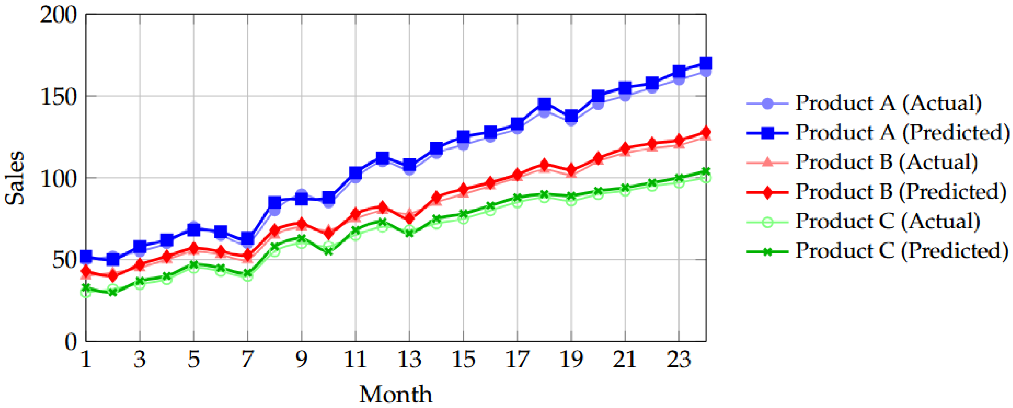
To illustrate the forecasting capability of the proposed Enhanced BiLSTM model, Figure 2 presents the predicted versus actual monthly sales for three representative products. The examples include periods with seasonal peaks, promotional events, and occasional sales spikes. The figure shows that the proposed model closely tracks actual sales trends and effectively captures fluctuations, demonstrating robustness in complex scenarios.

6.2. Model Component Evaluation

To quantify the contribution of each component in the proposed Enhanced BiLSTM model, a series of ablation experiments were conducted. The key modules considered include the adaptive attention mechanism, residual connections, and Bayesian hyperparameter optimization. Each component was systematically removed or replaced to assess its impact on forecasting performance, measured by RMSE, MAE, MAPE, and $R^2$.

The BiLSTM variant with residual connections but without the adaptive attention mechanism (BiLSTM + Residual) exhibits higher RMSE and MAPE compared to the full model, indicating that the attention module is essential for focusing on critical temporal features such as seasonal trends and promotional spikes. Removing residual connections while retaining the dual-activation attention module (BiLSTM + Attention) results in increased MAE and a slight decrease in $R^2$, demonstrating that residual connections help preserve feature representations and stabilize gradient flow during training. When all model components are included but Bayesian hyperparameter optimization is omitted (Enhanced BiLSTM w/o BO), the model shows slightly degraded RMSE and MAPE, highlighting the importance of automated hyperparameter tuning in achieving optimal generalization across diverse sales patterns. The standard BiLSTM without attention, residual connections, or Bayesian optimization serves as a baseline and shows the lowest predictive performance across all metrics.

Table 5. Ablation study results for Eenanced BiLSTM.

Model Variant	RMSE	MAE	MAPE (%)	${\mathit{R}}^2$
Base BiLSTM	16.5	12.6	10.9	0.84
BiLSTM + Residual	15.8	12.0	10.3	0.86
BiLSTM + Attention	15.2	11.9	10.1	0.87
Enhanced BiLSTM w/o BO	14.0	10.9	9.2	0.90
Proposed Enhanced BiLSTM	13.2	10.2	8.7	0.92

clearly shows the incremental contributions of each component. Introducing the adaptive attention mechanism reduces RMSE from 15.8 to 15.2 and MAPE from 10.3% to 10.1%, emphasizing its role in capturing relevant temporal dependencies. Adding residual connections further improves accuracy and stability, as reflected in the reduction of MAE to 11.9 and an increase of $R^2$ to 0.87. Incorporating Bayesian hyperparameter optimization allows the model to achieve its best performance, with RMSE of 13.2, MAE of 10.2, MAPE of 8.7%, and $R^2$ of 0.92, demonstrating that the full proposed Enhanced BiLSTM effectively integrates all modules to provide robust and accurate sales forecasts.

6.3. Hyperparameter Influence Evaluation

To examine how key hyperparameters affect the performance of the proposed Enhanced BiLSTM model, we conducted a series of sensitivity analyses. The hyperparameters considered include the learning rate, hidden-layer size, attention-layer dimension, and dropout rate. Each hyperparameter was varied within a reasonable range while keeping other parameters fixed to evaluate its effect on RMSE, MAE, MAPE, and $R^2$.

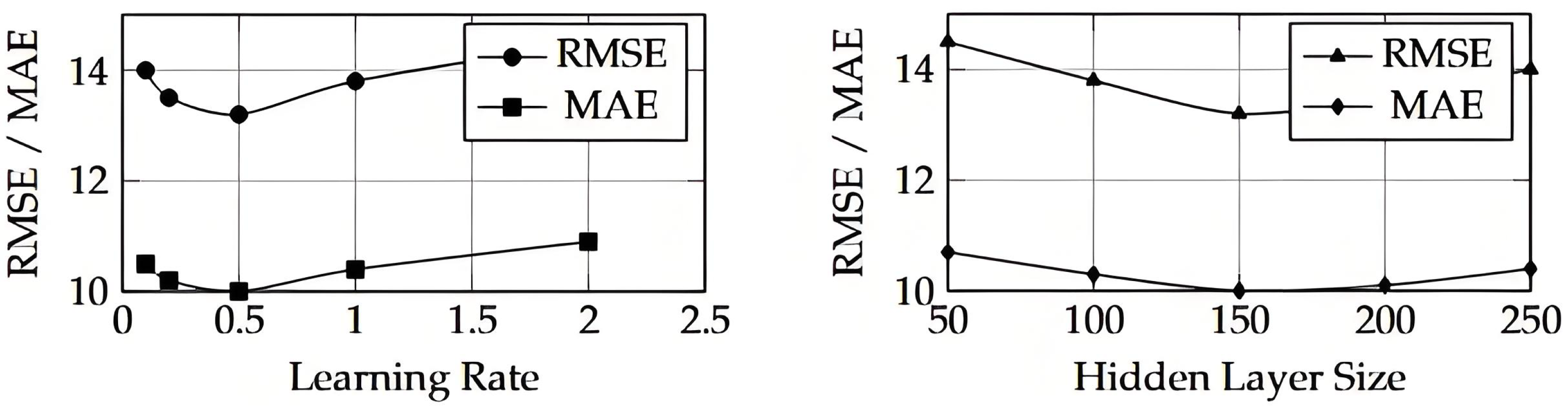
Figure 3 presents the relationship between selected hyperparameters and RMSE/MAE metrics. As shown, the model performance is sensitive to the choice of learning rate. A learning rate that is too large or too small leads to slower convergence or suboptimal solutions. Similarly, increasing the hidden layer size generally improves predictive accuracy up to a certain point, beyond which overfitting may occur. The attention layer dimension significantly affects the model’s ability to capture temporal dependencies, and an appropriately chosen dropout rate helps prevent overfitting while maintaining stable training.

These results highlight the importance of automated hyperparameter tuning. By employing Bayesian optimization, the model can efficiently search the hyperparameter space and identify configurations that achieve near-optimal forecasting performance, avoiding manual trial-and-error and ensuring robust generalization across diverse cross-border e-commerce datasets. To explore the effect of key hyperparameters on the performance of the proposed Enhanced BiLSTM model, we conducted a series of sensitivity analyses. The hyperparameters considered include the learning rate, hidden-layer size, attention-layer dimension, and dropout rate. Each hyperparameter was varied within a reasonable range while keeping other parameters fixed to evaluate its effect on RMSE, MAE, MAPE, and $R^2$.

Table 6. Effect of hyperparameter settings on model performance.

Hyperparameter	Learning Rate	Hidden Layer Size	Attention Layer Dimension	Dropout Rate	RMSE	MAE
Default Setting	0.001	128	64	0.2	13.2	10.2
Higher Learning Rate	0.01	128	64	0.2	14.5	11.0
Lower Learning Rate	0.0001	128	64	0.2	15.0	11.3
Larger Hidden Layer	0.001	256	64	0.2	13.5	10.5
Smaller Hidden Layer	0.001	64	64	0.2	14.0	11.0
Larger Attention Layer	0.001	128	128	0.2	13.0	10.0
Smaller Attention Layer	0.001	128	32	0.2	14.0	11.2
Higher Dropout Rate	0.001	128	64	0.4	13.5	10.6
Lower Dropout Rate	0.001	128	64	0.1	14.0	11.0

shows the effect of selected hyperparameters on RMSE and MAE. The model is sensitive to the learning rate. A learning rate that is too large or too small leads to slower convergence or suboptimal solutions. For example, 0.01 or 0.0001 increases both RMSE and MAE compared to 0.001. Increasing the hidden layer size to 256 slightly improves accuracy. A smaller size of 64 reduces performance. The attention layer dimension also matters. A larger layer of 128 improves results, while a smaller layer of 32 worsens them. Dropout affects stability. A rate of 0.2 works best. Higher (0.4) or lower (0.1) rates slightly reduce performance. These results highlight the importance of carefully selecting hyperparameters for optimal model performance.

These results highlight the importance of automated hyperparameter tuning. By employing Bayesian optimization, the model can efficiently search the hyperparameter space and identify configurations that achieve near-optimal forecasting performance, avoiding manual trial-and-error and ensuring robust generalization across diverse cross-border e-commerce datasets.

6.4. Training Time and Computational Efficiency Evaluation

Along with forecasting accuracy, the computational efficiency of the Enhanced BiLSTM model is vital for practical use in cross-border e-commerce. We evaluated the training time per epoch, inference time per sample, and total number of trainable parameters for the proposed model and all baseline algorithms.

Table 7. Computational efficiency comparison across models.

Model	Train Time/Epoch (s)	Inference Time/Sample (ms)	Parameters (M)
ARIMA	0.5	0.01	0.001
LSTM	12	0.15	1.2
BiLSTM	14	0.18	2.3
BiLSTM + Att	18	0.22	2.5
TCN	20	0.25	2.8
TFT	22	0.30	3.1
Enhanced BiLSTM	19	0.23	2.6

summarizes the results. Classical statistical models such as ARIMA have minimal parameter counts and fast computation but suffer from lower predictive accuracy. Standard LSTMs and BiLSTMs introduce additional parameters and require longer training times, whereas models with attention mechanisms and modern architectures, such as TCN and TFT, further increase computational cost. The proposed Enhanced BiLSTM strikes a balance by achieving high predictive performance with a moderate increase in parameters and training time. Its inference speed remains suitable for real-time or near-real-time forecasting, making it a practical choice for operational deployment.

These results demonstrate that although the Enhanced BiLSTM model introduces additional parameters due to the adaptive attention and residual modules, the computational overhead remains moderate. The model maintains reasonable training and inference times while delivering superior predictive performance, confirming its suitability for practical cross-border e-commerce forecasting tasks.

6.5. Effect of Sequence Length/Time Window

The length of the input sequence, or historical observation window, can significantly impact forecasting performance in cross-border e-commerce sales. Short windows may miss long-term trends or seasonal patterns, while overly long windows can introduce noise and increase computational cost. To investigate this, we evaluated the Enhanced BiLSTM model using different time windows: 3 months, 6 months, and 12 months of historical sales data.

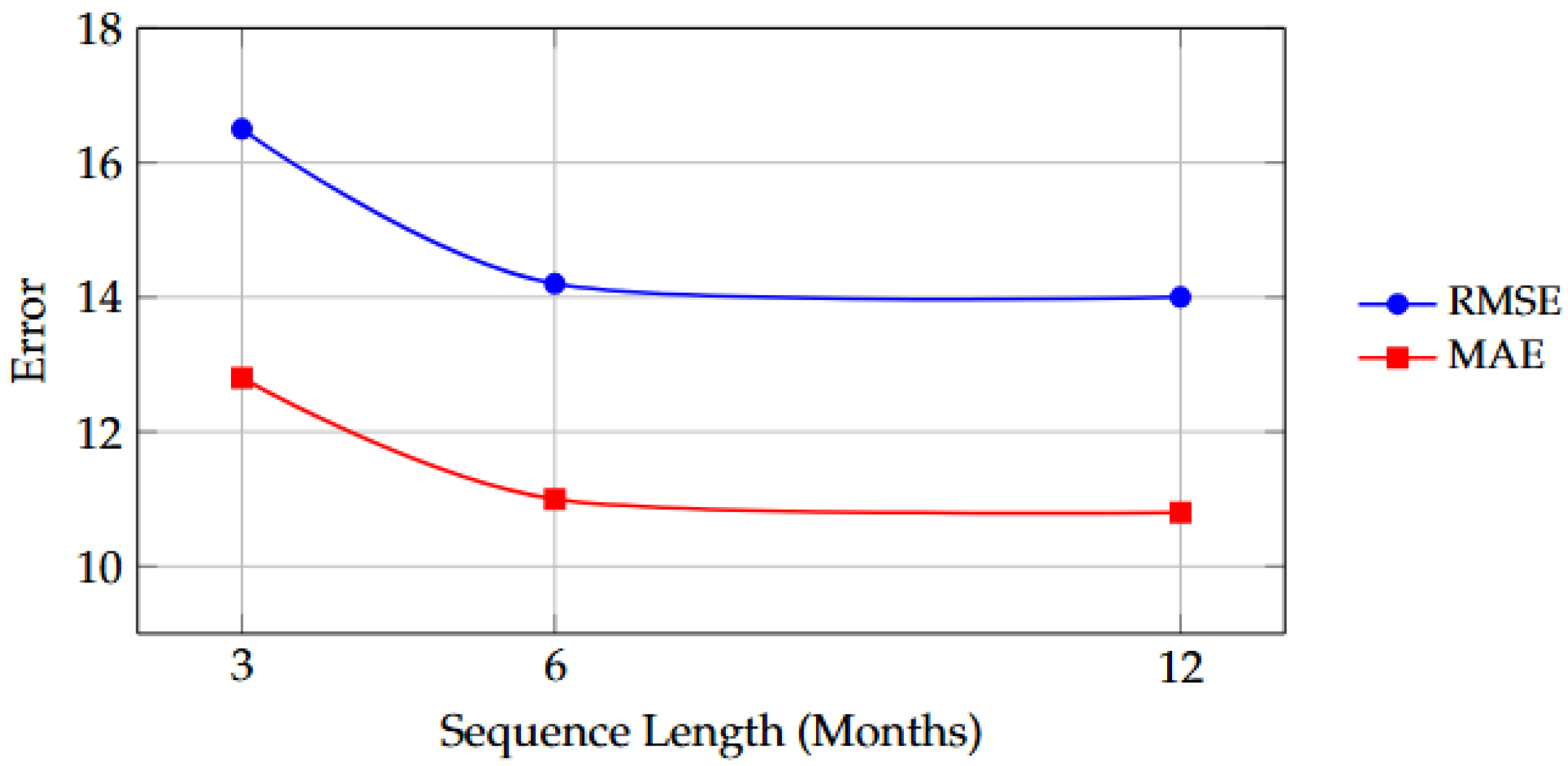
Figure 4 shows the RMSE and MAE for each window length. The results indicate that a 6-month window generally provides the best trade-off, capturing both short-term fluctuations and seasonal trends without overfitting. Shorter windows (3 months) fail to capture recurring seasonal effects, leading to higher RMSE and MAPE, whereas longer windows (12 months) yield only marginal improvement but increase model complexity. These results emphasize the importance of choosing an appropriate sequence length to balance short-term responsiveness and long-term pattern recognition in cross-border e-commerce sales forecasting.

Additionally,

Table 8. Impact of sequence length on model performance.

Sequence Length	RMSE	MAE	MAPE (%)
3 months	16.2	12.8	11.2
6 months	13.2	10.2	8.7
12 months	13.0	10.1	8.5

presents a summary of the performance metrics (RMSE, MAE, and MAPE) for each sequence length. It shows that the 6-month window achieves the best performance in terms of both RMSE and MAPE, further confirming the findings from the figure.

7. Conclusions

This study proposes an enhanced BiLSTM model for cross-border e-commerce sales forecasting, which integrates bidirectional temporal modeling, an adaptive attention mechanism, and Bayesian optimization for hyperparameter tuning. The model overcomes the limitations of traditional time-series models and existing deep learning approaches, effectively capturing complex nonlinear sales patterns, seasonality, and demand fluctuations. The following conclusions are drawn from the experimental results:

• The model outperforms six baseline models, achieving a RMSE of 13.2, MAE of 10.2, MAPE of 8.7%, and a coefficient of R² of 0.92, demonstrating its superior accuracy in cross-border e-commerce sales forecasting.
• Ablation studies show the contribution of each component: the adaptive attention mechanism improves prediction accuracy, residual connections reduce errors, and Bayesian optimization enhances overall model performance.
• The model strikes an effective balance between performance and computational efficiency. With fast training and inference times, it demonstrates practicality for real-world deployment, making it suitable for large-scale, real-time forecasting tasks.

Despite these advantages, the model has some limitations. It relies solely on historical sales data and does not incorporate external factors such as macroeconomic indicators or social media sentiment, which may impact demand forecasting in cross-border e-commerce. The fixed input sequence length may also not be optimal for products with irregular demand patterns, and scalability challenges may arise in large-scale e-commerce platforms.

Future work will address these limitations by integrating multi-source data, adapting the model to specific product categories, and exploring dynamic attention mechanisms. We also plan to optimize the model for large-scale deployment and test it on a wider range of cross-border e-commerce datasets. Additionally, we will explore Transformer-based models to handle longer datasets and capture global dependencies more effectively.

References

1. Qi, K.; Wu, W.; Ni, Y. SymOpt-CNSVR: A Novel Prediction Model Based on Symmetric Optimization for Delivery Duration Forecasting. Symmetry 2025, 17, 1608. [Google Scholar]
2. Zhu, L.; Liu, W.; Tan, H.; Hu, T. A novel Bayesian optimization prediction framework for four-axis industrial robot joint motion state. Complex Intell. Syst. 2024, 10, 4867–4881. [Google Scholar] [CrossRef]
3. Gong, Z. Optimization of cross-border E-commerce (CBEC) supply chain management based on fuzzy logic and auction theory. Sci. Rep. 2024, 14, 14088. [Google Scholar]
4. Li, J.; Li, J.; Li, J.; Zhang, G. Bayesian-Optimized GCN-BiLSTM-Adaboost Model for Power-Load Forecasting. Electronics 2025, 14, 3332. [Google Scholar]
5. Guo, X.; Mo, Y.; Yan, K. Short-Term Photovoltaic Power Forecasting Based on Historical Information and Deep Learning Methods. Sensors 2022, 22, 9630. [Google Scholar] [CrossRef]
6. Kwon, H.; Do, T.N.; Won, W.; Kim, J. An optimization model for the market-responsive operation of naphtha cracking process with price prediction. Chem. Eng. Res. Des. 2022, 188, 681–693. [Google Scholar] [CrossRef]
7. Lou, G.; Lin, W.; Huang, G.; Xiang, W. A two-stage online remaining useful life prediction framework for supercapacitors based on the fusion of deep learning network and state estimation algorithm. Eng. Appl. Artif. Intell. 2023, 123, 106399. [Google Scholar] [CrossRef]
8. Gena, X.; Zhang, Y. Sales Forecasting using ARIMA Models: A Case Study in the Retail Industry. J. Retail Anal. 2015, 12, 45–56. [Google Scholar]
9. Rostan, P.; Rostan, A.; Nurunnabi, M. Options Trading Strategy Based on ARIMA Forecasting. PSU Res. Rev. 2020, 4, 111–127. [Google Scholar] [CrossRef]
10. Wang, P.; Xu, Z. A Novel Consumer Purchase Behavior Recognition Method Using Ensemble Learning Algorithm. Math. Probl. Eng. 2020, 2020, 6673535. [Google Scholar] [CrossRef]
11. Cho, M.; Kim, C.; Jung, K.; Jung, H. Water Level Prediction Model Applying a Long Short-Term Memory (LSTM)—Gated Recurrent Unit (GRU) Method for Flood Prediction. Water 2022, 14, 2221. [Google Scholar] [CrossRef]
12. Tsai, P.-F.; Gao, C.-H.; Yuan, S.-M. Stock Selection Using Machine Learning Based on Financial Ratios. Mathematics 2023, 11, 4758. [Google Scholar] [CrossRef]
13. Khandelwal, V.; Chaturvedi, A.K.; Gupta, C.P. Amazon EC2 Spot Price Prediction Using Regression Random Forests. IEEE Trans. Cloud Comput. 2020, 8, 59–72. [Google Scholar] [CrossRef]
14. Qin, C.; Chen, L.; Cai, Z.; Liu, M.; Jin, L. Long short-term memory with activation on gradient. Neural Netw. 2023, 164, 135–145. [Google Scholar] [CrossRef]
15. Su, Y.; Kuo, C.-C.J. On extended long short-term memory and dependent bidirectional recurrent neural network. Neurocomputing 2019, 356, 151–161. [Google Scholar] [CrossRef]
16. Bahdanau, D.; Cho, K.; Bengio, Y. Neural machine translation by jointly learning to align and translate. In Proceedings of the International Conference on Learning Representations (ICLR), San Diego, CA, USA, 7–9 May 2015. [Google Scholar]
17. Snoek, J.; Larochelle, H.; Adams, R.P. Practical Bayesian optimization of machine learning algorithms. In Proceedings of the Advances in Neural Information Processing Systems (NeurIPS), Lake Tahoe, NV, USA, 3–8 December 2012; Volume 25, pp. 2951–2959. [Google Scholar]
18. Li, G.; Li, N. Customs classification for cross-border e-commerce based on text-image adaptive convolutional neural network. Electron. Commer. Res. 2019, 19, 779–800. [Google Scholar]
19. Jiang, C. Research on sales forecasting and consumption recommendation system of e-commerce agricultural products based on LSTM model. GeoJournal 2025, 90, 93. [Google Scholar] [CrossRef]
20. Li, J.; Pan, Y.; Yang, Y.; Tse, C.H. Digital platform attention and international sales: An attention-based view. J. Int. Bus. Stud. 2022, 53, 1817–1835. [Google Scholar] [CrossRef]
21. Singh, K.; Booma, P.M.; Eaganathan, U. E-commerce system for sale prediction using machine learning technique. J. Phys. Conf. Ser. 2020, 1712, 012042. [Google Scholar] [CrossRef]
22. He, M.; Zhuang, L.; Yang, S.; Xu, Z.; Li, W.; Lu, J. An energy-efficient VNE algorithm based on bidirectional long short-term memory. J. Netw. Syst. Manag. 2022, 30, 45. [Google Scholar] [CrossRef]
23. Jürgensmeier, L.; Bischoff, J.; Skiera, B. Opportunities for self-preferencing in international online marketplaces. Int. Mark. Rev. 2024, 41, 1118–1132. [Google Scholar] [CrossRef]
24. Gers, F.A.; Schmidhuber, J.; Cummins, F. Learning to forget: Continual prediction with LSTM. Neural Comput. 2000, 12, 2451–2471. [Google Scholar] [CrossRef] [PubMed]
25. Hochreiter, S.; Schmidhuber, J. Long Short-Term Memory. Neural Comput. 1997, 9, 1735–1780. [Google Scholar] [CrossRef] [PubMed]
26. Bai, S.; Zhuang, F.; He, X. An empirical evaluation of generic convolutional and recurrent networks for sequence modeling. In Proceedings of the International Conference on Learning Representations (ICLR 2019), New Orleans, LA, USA, 6–9 May 2019. [Google Scholar]
27. Lim, B.; Arık, S.Ö.; Loeff, N.; Pfister, T. Temporal Fusion Transformers for interpretable multi-horizon time series forecasting. Int. J. Forecast. 2021, 37, 1748–1764. [Google Scholar] [CrossRef]
Figure 1. The overall framework of the proposed enhanced BiLSTM model for cross-border e-commerce sales forecasting.
Mca 31 00017 g001
Figure 2. Prediction examples for selected products, showing actual vs. predicted sales over 24 months.
Mca 31 00017 g002
Figure 3. Sensitivity analysis of key hyperparameters on RMSE and MAE for the Enhanced BiLSTM model.
Mca 31 00017 g003
Figure 4. Effect of input sequence length on forecasting performance for the Enhanced BiLSTM model.
Mca 31 00017 g004