Article

Theory of Functional Connections Extended to Continuous Integral Constraints

Aerospace Engineering, Texas A&M University, College Station, TX 77843, USA
Math. Comput. Appl. 2025, 30(5), 105; https://doi.org/10.3390/mca30050105
Submission received: 21 August 2025 / Revised: 22 September 2025 / Accepted: 23 September 2025 / Published: 24 September 2025
(This article belongs to the Section Engineering)

Abstract

This study extends the Theory of Functional Connections, previously applied to constraints specified at discrete points, to encompass continuous integral constraints of the form x 0 x f f ( x , t ) d x = I ( t ) , where I ( t ) can be a constant, a prescribed function, or an unknown function to be estimated through optimization. The framework of continuous integral constraints is developed within the context of initial value problems (IVP) and boundary value problems (BVP). To demonstrate the effectiveness of this analytical approach, examples validate the method and highlight distinctions between satisfying continuous integral constraints via simple interpolation versus functional interpolation. A limitation of the proposed approach is the inability to inherently enforce inequality constraints, such as the positivity constraint f ( x , t ) 0 , for modeling probability density functions in classical mechanics. Despite this, numerical experiments on boundary-value problems rarely result in negative values, indicating that the issue occurs infrequently. However, a mitigation strategy based on non-negative least-squares methods combined with Bernstein polynomials is proposed to address these rare cases. This approach is validated through an additional numerical test, demonstrating its efficacy in ensuring nonnegativity when required.

1. Introduction

The Theory of Functional Connections (TFC), introduced in [1,2], then expanded in [3,4], and summarized in [5], generalizes the traditional interpolation problem—where a function is constructed using n linearly independent support functions to satisfy n constraints—into the broader functional interpolation problem. This framework aims to find a functional representing the entire set of interpolation functions satisfying a given set of n constraints. These functionals define the subspace of functions that satisfy the constraints, effectively narrowing the solution space to the region where the solution to a constrained optimization problem resides. By utilizing these functionals, constrained optimization problems are transformed into unconstrained ones, enabling solutions through simpler, more robust, accurate, faster, and more reliable methods. This means that TFC can turn problems with constraints into unconstrained ones in a way that may make them easier to solve.
The seminal paper [1] has shown how to address univariate constraints involving points, derivatives, and any linear combination of these. The theory was then extended to accommodate integral, infinite, and multivariate constraints and applied to solving ordinary, partial, and integrodifferential equations. The univariate version of TFC can be expressed in one of the following two forms:
f x , g ( x ) = g ( x ) + j = 1 n η j x , g ( x ) s j ( x ) f x , g ( x ) = g ( x ) + j = 1 n ϕ j x , s ( x ) ρ j x , g ( x ) ,
where n represents the number of linear constraints, g ( x ) is the free function, and s j ( x ) are n user-defined, linearly independent support functions. The terms η j ( x , g ( x ) ) are the coefficient functionals, ϕ j ( x ) are switching functions (which take a value of 1 when evaluated at their respective constraint and 0 at other constraints), and ρ j x , g ( x ) are projection functionals that express the constraints in terms of the free function. Detailed explanations and properties of these elements are provided in [3,4,5] and will be applied in this article without further justification.
Since the publication of [1], numerous applications and extensions of TFC have emerged, demonstrating its versatility across various fields. These applications include the extension to shear-type and mixed derivatives [6], an easy representation of any fractional operator [7,8], how to solve geodesic boundary value problems in curved spaces [9], and an extension of continuation methods [10]. Furthermore, TFC has been applied to indirect optimal control [11,12], modeling stiff chemical kinetics [13], and studying epidemiological dynamics [14]. It also shows promise in nonlinear programming [15] and structural mechanics [16,17], among other areas. Applying TFC in neural networks has proven particularly efficient [18,19], especially regarding the accuracy and the capacity to address high-dimensional problems. Notably, TFC enhances the performance of Physics-Informed Neural Networks [20,21] by effectively removing constraints from the optimization process, which traditional neural networks struggle to incorporate. This capability allows the class of neural networks to improve computational efficiency and accuracy in solving complex problems.
At first glance, TFC and spectral methods may appear similar in their approach to solving differential equations and constrained optimization problems. However, two key differences set them apart: (1) Spectral methods express the solution itself as a sum of basis functions, while TFC uses this representation for the free function. This distinction enables TFC to analytically enforce constraints within its formulation, whereas spectral methods treat constraints as supplementary data, approximating their satisfaction based on the accuracy of the residuals. (2) For linear boundary value problems, the computational strategies differ significantly. Spectral methods often rely on iterative techniques, such as the shooting method, to transform the BVP into an equivalent IVP for ease of computation. In contrast, TFC directly tackles BVPs using linear least-squares methods, thereby eliminating the need for iterative procedures. Both methodologies can incorporate optimization through either the Galerkin method, which ensures orthogonality between the residual vector and the selected basis functions, or the Collocation method, which minimizes the residual vector’s norm.
There are distinctions also with the Lagrange multiplier method for enforcing constraints in optimization problems. The Lagrange multiplier method introduces auxiliary variables–the multipliers–which must be calculated to satisfy the imposed constraints; while the computation of the multipliers is relatively straightforward in certain scenarios, it can become highly complex or even practically unmanageable in others, significantly increasing the problem’s difficulty. In contrast, TFC avoids the introduction of additional variables and facilitates the derivation of constrained functionals without encountering such computational challenges. However, a notable limitation of TFC is its current inability to handle inequality constraints, a domain where the Lagrange multiplier method excels. Both methods share a common drawback: they are prone to identifying solutions that correspond to local optima rather than guaranteeing global optima, particularly in the case of non-convex problems. As a result, supplementary verification techniques or alternative optimization methods may be necessary to ensure the global validity and quality of the obtained solutions. In conclusion, while TFC does not entirely supplant the Lagrange multiplier method, it offers a compelling alternative in scenarios where the computation of multipliers is prohibitively complex or infeasible, provided the constraints are restricted to equalities.
Appendix B of Ref. [5] addresses one particularly noteworthy unresolved problem: the development of an “integral-preserving” functional. The ability to derive such a functional would mark a significant advancement, facilitating the establishment of methodologies aimed at ensuring the preservation of an integral condition. This aspect emphasizes the crucial nature of integral constraints, which assure physical, mathematical, and practical coherence in systems characterized by fundamental conservation principles or cumulative properties. The ability to derive a continuous integral functional is essential for the effective resolution of stochastic differential equations, including the Fokker–Planck equation. This article proposes a solution to this challenge and extends the work of TFC by deriving continuous integral-constrained functionals. These newly developed functionals are not only well-suited for enforcing integral-preserving constraints but also extend their applicability to cases where the integral constraint is assigned and not constant or to cases where it is an unknown function that must be determined as part of an optimization process.
In the next section, an integral invariant functional is derived using the “ η ” formulation for an IVP and the “switching-projection” formulation for BVP.

2. Integral Invariant Functionals

Integral invariant scenarios, commonly referred to as conservation laws or integrability conditions, describe situations in which specific quantities remain unchanged or invariant over time despite the dynamic evolution of the system. These conditions are fundamental in various scientific and mathematical disciplines, as they reflect the inherent symmetries and structure of natural laws. For instance, in physics, the conservation of energy asserts that the total energy of a closed system is constant, regardless of internal changes. In fluid dynamics, the conservation of mass ensures that mass cannot be created or destroyed, while in electromagnetism, the conservation of charge governs the behavior of electric and magnetic fields. Similarly, in mechanics, both linear and angular momentum are conserved under certain conditions, underpinning the motion of objects in fields such as astronomy and classical mechanics. Likewise, the conservation of probability in both classical and quantum mechanics guarantees that the likelihood of all possible outcomes sums to one, preserving the predictability and consistency of the system’s behavior.
The next subsection shows how to obtain constrained functionals that can be used in stochastic differential equations and optimization problems when considering initial value problems. The purpose is to derive a functional, f x , t , g ( x , t ) , that analytically satisfies the integral constraint,
x 0 x f f x , t , g ( x , t ) d x = 1 ,
for any time t [ t 0 , t f ] and for any expression of the free function, g ( x , t ) . The optimal free function minimizing the optimization problem will be found by expanding it as a linear combination of orthogonal polynomials (as performed in [2,22] to solve ordinary differential equations by least-squares) or as a single-layer feed-forward neural network by machine learning, as performed in [14,19].

2.1. Constrained Functionals for Initial Value Problems

Let us consider deriving a functional, f x , t , g ( x , t ) , where ( x , t ) [ x 0 , x f ] × [ t 0 , t f ] , subject to the x-constraints,
f ( x 0 , t ) = b 0 ( t ) and f ( x f , t ) = b f ( t ) ,
and to the (initial) time value problem (constraint),
f ( x , t 0 ) = f 0 ( x ) ,
satisfying x 0 x f f 0 ( x ) d x = 1 .
Equations (1) and (2) represent three constraints. These constraints must be consistent. This means they must satisfy,
f 0 ( x 0 ) = b 0 ( t 0 ) and f 0 ( x f ) = b f ( t 0 ) .
Using monomials as support functions, s ( x ) : = { 1 , x , x 2 } , the support matrix for these constraints is,
B = s 1 ( x 0 ) s 2 ( x 0 ) s 3 ( x 0 ) s 1 ( x f ) s 2 ( x f ) s 3 ( x f ) x 0 x f s 1 ( τ ) d τ x 0 x f s 2 ( τ ) d τ x 0 x f s 3 ( τ ) d τ = 1 x 0 x 0 2 1 x f x f 2 x f x 0 x f 2 x 0 2 2 x f 3 x 0 3 3 .
The inverse of this matrix,
B 1 = x f ( x f + 2 x 0 ) ( x 0 x f ) 2 x 0 ( x 0 + 2 x f ) ( x 0 x f ) 2 6 x 0 x f ( x 0 x f ) 3 2 ( x 0 + 2 x f ) ( x 0 x f ) 2 2 ( x f + 2 x 0 ) ( x 0 x f ) 2 6 ( x 0 + x f ) ( x 0 x f ) 3 3 ( x 0 x f ) 2 3 ( x 0 x f ) 2 6 ( x 0 x f ) 3 = c 11 c 12 c 13 c 21 c 22 c 23 c 31 c 32 c 33
provides the coefficients of the switching functions,
ϕ 1 ( x ) = c 11 + c 21 x + c 31 x 2 ϕ 2 ( x ) = c 12 + c 22 x + c 32 x 2 ϕ 3 ( x ) = c 13 + c 23 x + c 33 x 2 ,
while the projection functionals are,
ρ 1 ( t ) = b 0 ( t ) g ( x ) ( x 0 , t ) , ρ 2 ( t ) = b f ( t ) g ( x ) ( x f , t ) , and ρ 3 ( t ) = 1 x 0 x f g ( x ) ( x , t ) d x .
Therefore, using the TFC switching-projection formulation [5], the constrained functional for the x-constraints is,
f ( x ) x , t , g ( x ) ( x , t ) = g ( x ) ( x , t ) + ϕ 1 ( x ) b 0 ( t ) g ( x ) ( x 0 , t ) + ϕ 2 ( x ) b f ( t ) g ( x ) ( x f , t ) + ϕ 3 ( x ) 1 x 0 x f g ( x ) ( x , t ) d x
while the constrained functional for the t-constraint, given in Equation (3), is,
f ( t ) x , t , g ( t ) ( x , t ) = g ( t ) ( x , t ) + f 0 ( x ) g ( t ) ( x , t 0 ) .
The overall constrained functional (satisfying all constraints) is then obtained by replacing the free function, g ( x ) ( x , t ) , in Equation (5), with the expression of f ( t ) x , t , g ( t ) ( x , t ) , provided by Equation (6). Removing the superscripts, we then obtain,
f x , t , g ( x , t ) = g ( x , t ) + f 0 ( x ) g ( x , t 0 ) + ϕ 3 ( x ) 1 x 0 x f g ( x , t ) + f 0 ( x ) g ( x , t 0 ) d x + ϕ 1 ( x ) b 0 ( t ) g ( x 0 , t ) f 0 ( x 0 ) + g ( x 0 , t 0 ) + ϕ 2 ( x ) b f ( t ) g ( x f , t ) f 0 ( x f ) + g ( x f , t 0 )

Numerical Validation

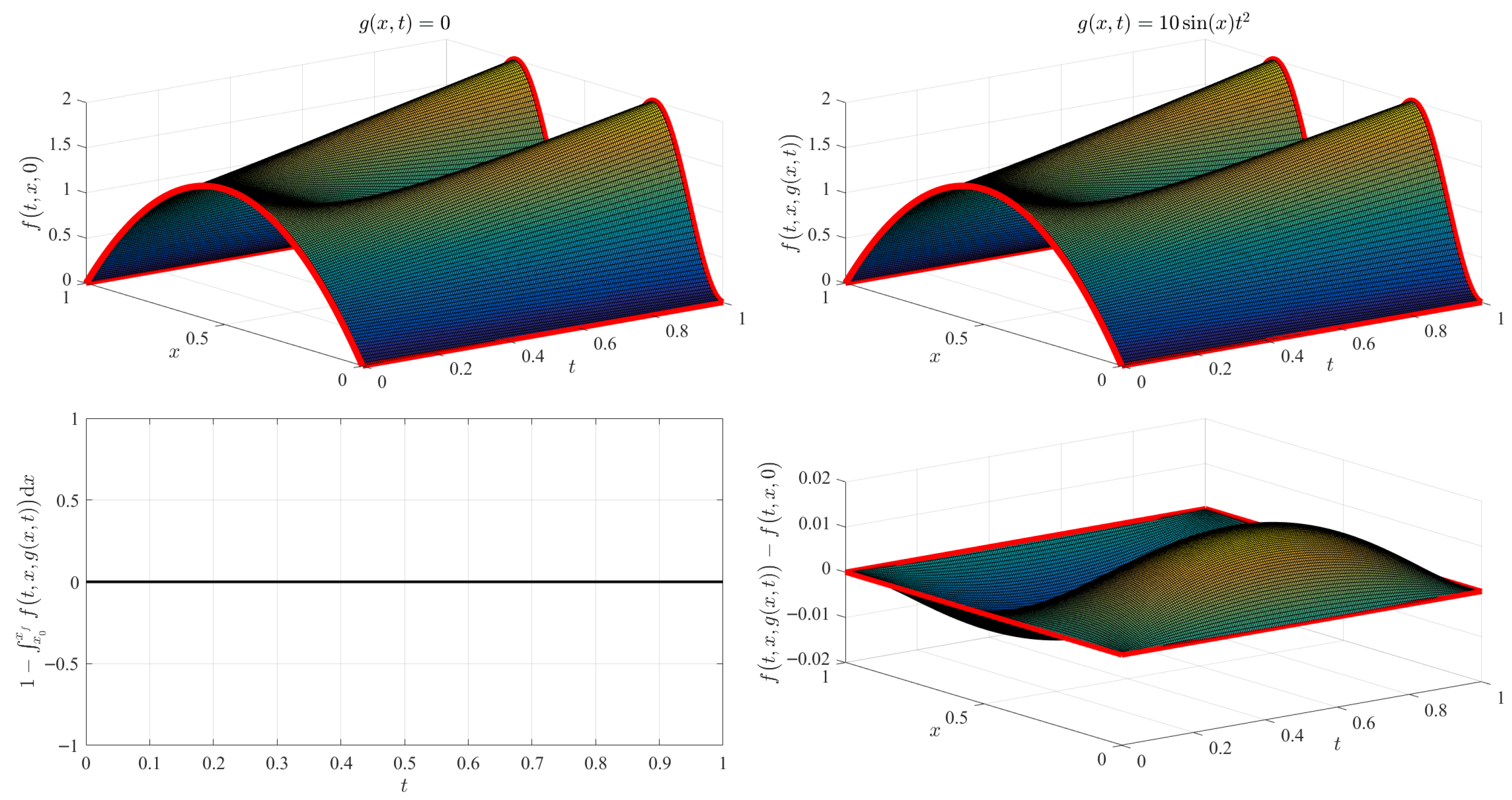
Equation (7) is numerically tested for the following conditions: x 0 = 0 , x f = 1 , t 0 = 0 , and t f = 1 , while the initial function, f ( x , t 0 ) = 6 ( 1 x ) x , has been selected consistent with the integral invariant constraint to 1. The side boundary functions are selected as b 0 ( t ) = sin t and b f ( t ) = t ( 1 t ) . The domain has been discretized by 201 uniformly distributed points in both coordinates, x and t.
The results of the numerical tests are shown in Figure 1. The surface obtained by Equation (7) using g ( x , t ) = 0 is shown in the top-left plot. Setting g ( x , t ) = 0 implies obtaining the interpolation surface for the support functions selected. Using the same support functions and g ( x , t ) = ( 1 + x ) t 2 , the surface shown in the top-center plot is obtained. This surface represents the functional interpolation surface for the given free function. The difference between these two surfaces is provided in the top-right plot, where the variational effect provided by the free function can be better appreciated. This plot clearly shows that the boundary constraints are analytically satisfied, with a zero difference (shown in red). The full respect of the side boundary functions is shown in the bottom-left and bottom-right plots, respectively. For the surface with the free function, g ( x , t ) = ( 1 + x ) t 2 , the time-invariant integral (estimated by the Simpson method) is shown in the bottom-center plot, showing the analytical satisfaction of the integral at any time.
In an initial-value optimization problem, such as in a differential equation satisfying the constraints given in Equations (2) and (3), there will be an optimal free function making the constrained functional satisfy the differential equation. By expanding the free function in terms of a set of basis functions, such as orthogonal polynomials or neural networks, the optimal coefficients of the expansion can be determined by minimizing the residuals of the differential equation.

2.2. Constrained Functionals for Boundary Value Problems

For boundary-value problems, the x-constraints are provided, as for the initial value problems, by Equations (1) and (2). Therefore, the associate constrained functional, given by Equation (5), remains the same while the t-constraints become,
f ( x , t 0 ) = f 0 ( x ) and f ( x , t f ) = f f ( x )
Equation (8) represents two constraints that must be consistent with constraints given in Equation (1). This means that, in addition to the conditions provided in Equation (4), they also must satisfy,
f f ( x 0 ) = b 0 ( t f ) and f f ( x f ) = b f ( t f )
The corresponding constrained functional, satisfying these two constraints and replacing Equation (6) is,
f ( t ) x , t , g ( t ) ( x , t ) = g ( t ) ( x , t ) + t t f t 0 t f f 0 ( x ) g ( t ) ( x , t 0 ) + t t 0 t f t 0 f f ( x ) g ( t ) ( x , t f )
The global constrained functional is obtained by substituting the constrained functional in t provided by Equation (9), into the free function g ( x ) ( x , t ) of Equation (5) or the constrained functional in x, Equation (5), into the free function g ( t ) ( x , t ) given in Equation (9). Removing the superscripts, we obtain,
f x , t , g ( x , t ) = g ( x , t ) + t t f t 0 t f f 0 ( x ) g ( x , t 0 ) + t t 0 t f t 0 f f ( x ) g ( x , t f ) + ϕ 1 ( x ) b 0 ( t ) g ( x 0 , t ) t t f t 0 t f f 0 ( x 0 ) g ( x 0 , t 0 ) t t 0 t f t 0 f f ( x 0 ) g ( x 0 , t f ) + ϕ 2 ( x ) b f ( t ) g ( x f , t ) t t f t 0 t f f 0 ( x f ) g ( x f , t 0 ) t t 0 t f t 0 f f ( x f ) g ( x f , t f ) + ϕ 3 ( x ) 1 x 0 x f g ( x , t ) + t t f t 0 t f f 0 ( x ) g ( x , t 0 ) + t t 0 t f t 0 f f ( x ) g ( x , t f ) d x

Numerical Validation

Equation (10) is numerically tested for the following conditions: x [ 0 , 1 ] , and t [ 0 , 1 ] , while the initial and final functions, f 0 ( x , t 0 ) = 6 ( 1 x ) x and f f ( x , t f ) = 1 cos ( 4 π x ) , have been selected to be consistent with the integral invariant to 1. The side boundary functions are selected simply as b 0 ( t ) = b f ( t ) = 0 . The domain is discretized in 201 uniformly distributed points in x and in t.
The results of the numerical tests are shown in Figure 2. The surface obtained by Equation (10) using g ( x , t ) = 0 is shown in the top-left plot. This surface represents the interpolation surface when using the specified support functions. Using the same support functions and g ( x , t ) = ( 1 + x ) t 2 , the surface shown in the top-right plot is obtained. This surface represents the functional interpolation surface for the given free function. The difference between these two surfaces is provided in the bottom-right plot, where the variational effect provided by the free function can now be appreciated. This plot clearly shows that the boundary constraints are identical with a zero difference (in red). The time-invariant integral is shown (for the surface with the free function g ( x , t ) = ( 1 + x ) t 2 ) in the bottom-left plot, showing the analytical satisfaction of the integral at any time.
It is important to outline that, while Equations (7) and (10) analytically satisfy the integral-preserving constraint, these constrained functionals do not guarantee the positivity constraint that a probability density function must satisfy. However, extensive numerical examples have been tested using the same constraints with different free-function expressions. The resulting surfaces rarely experienced negative values. When it occurs, it always happens close to the x-bounds and in connection with non-smooth free functions, highly differing from g ( t , x ) = 0 , which is associated with the interpolation case.
The mathematical challenge of addressing negative values in the solution has yet to be fully resolved. However, in the final section of this paper, we propose a novel method to mitigate this issue. Our approach involves approximating the optimal probability density function (pdf), which may take on negative values, using a series expansion composed exclusively of positive functions. Specifically, we employ two sets of positive functions: Gaussian mixtures or Bernstein polynomials. By representing the function in this way, we can apply a non-negative least-squares technique to ensure that the resulting coefficients remain positive, thereby producing an approximation that avoids the occurrence of negative values.

3. Time-Varying Integral Constrained Functionals

This section shows how to derive a constrained functional, f x , t , g ( x , t ) , where ( x , t ) [ x 0 , x f ] × [ t 0 , t f ] , subject to consistent (Dirichlet) boundary constraints and the additional constraint of a prescribed time-varying integral, J t , p ( t ) . The Dirichlet constraints are,
f x 0 , t , g ( x 0 , t ) = f ( x 0 , t ) f x f , t , g ( x f , t ) = f ( x f , t ) and f x , t 0 , g ( x , t 0 ) = f ( x , t 0 ) f x , t f , g ( x , t f ) = f ( x , t f )
while the assigned (or unknown) time-varying integral satisfies,
x 0 x f f x , t , g ( x , t ) d x = J ( t )
where J ( t ) can be any function subject to the consistency constraints,
J ( t 0 ) = x 0 x f f ( x , t 0 ) d x and J ( t f ) = x 0 x f f ( x , t f ) d x .
When the function J ( t ) is unknown, it must be determined through an optimization process. In such cases, the function can be represented by the constrained functional form,
J t , p ( t ) = p ( t ) + t t f t 0 t f J ( t 0 ) p ( t 0 ) + t t 0 t f t 0 J ( t f ) p ( t f )
functional satisfying the two constraints in Equation (11) and where p ( t ) is the free function that is estimated by the optimization process.
Following Ref. [5], Equation (11) represent two constraints in the t-variable,
f ( x , t 0 ) and f ( x , t f ) .
Then, using support functions s ( t ) : = { 1 , t } and the “switching-projection” TFC formulation, the associated constrained functional is,
f ( t ) x , t , g ( t ) ( x , t ) = g ( t ) ( x , t ) + t t f t 0 t f f ( x , t 0 ) g ( t ) ( x , t 0 ) + t t 0 t f t 0 f ( x , t f ) g ( t ) ( x , t f )
The constraints in the x-variable are,
f ( x 0 , t ) , f ( x f , t ) , and x 0 x f f ( x , t ) d x = J t , p ( t ) .
Again, using the support functions, s ( x ) : = 1 , x , x 2 and the “ η ” TFC formulation [5], the corresponding associated constrained functional has the form,
f ( x ) x , t , g ( x ) ( x , t ) = g ( x ) ( x , t ) + η 1 ( t ) + η 2 ( t ) x + η 3 ( t ) x 2
Imposing the constraints,
f ( x 0 , t ) = g ( x ) ( x 0 , t ) + η 1 ( t ) + η 2 ( t ) x 0 + η 3 ( t ) x 0 2 f ( x f , t ) = g ( x ) ( x f , t ) + η 1 ( t ) + η 2 ( t ) x f + η 3 ( t ) x f 2 J t , p ( t ) = x 0 x f g ( x ) ( x , t ) d x + η 1 ( t ) ( x f x 0 ) + η 2 ( t ) x f 2 x 0 2 2 + η 3 ( t ) x f 3 x 0 3 3
the linear system,
1 x 0 x 0 2 1 x f x f 2 x f x 0 x f 2 x 0 2 2 x f 3 x 0 3 3 η 1 ( t ) η 2 ( t ) η 3 ( t ) = f ( x 0 , t ) g ( x ) ( x 0 , t ) f ( x f , t ) g ( x ) ( x f , t ) J t , p ( t ) x 0 x f g ( x ) ( x , t ) d x
is obtained, which allows us to compute the η k ( t ) coefficients. The inverse of the coefficients’ matrix is,
c 11 c 12 c 13 c 21 c 22 c 23 c 31 c 32 c 33 = 1 x 0 x 0 2 1 x f x f 2 x f x 0 x f 2 x 0 2 2 x f 3 x 0 3 3 1 = x f ( x f + 2 x 0 ) ( x 0 x f ) 2 x 0 ( x 0 + 2 x f ) ( x 0 x f ) 2 6 x 0 x f ( x 0 x f ) 3 2 ( x 0 + 2 x f ) ( x 0 x f ) 2 2 ( x f + 2 x 0 ) ( x 0 x f ) 2 6 ( x 0 + x f ) ( x 0 x f ) 3 3 ( x 0 x f ) 2 3 ( x 0 x f ) 2 6 ( x 0 x f ) 3
Therefore, the η k ( t ) coefficients are,
η 1 ( t ) = c 11 f ( x 0 , t ) g ( x ) ( x 0 , t ) + c 12 f ( x f , t ) g ( x ) ( x f , t ) + c 13 J t , p ( t ) x 0 x f g ( x ) ( x , t ) d x η 2 ( t ) = c 21 f ( x 0 , t ) g ( x ) ( x 0 , t ) + c 22 f ( x f , t ) g ( x ) ( x f , t ) + c 23 J t , p ( t ) x 0 x f g ( x ) ( x , t ) d x η 3 ( t ) = c 31 f ( x 0 , t ) g ( x ) ( x 0 , t ) + c 32 f ( x f , t ) g ( x ) ( x f , t ) + c 33 J t , p ( t ) x 0 x f g ( x ) ( x , t ) d x
The final constrained functional is then obtained using the TFC recursive approach [5] by substituting the free function, g ( x ) ( x , t ) , appearing in Equation (13) and in the η k ( t ) coefficients in Equation (14), by the constrained functional, f ( t ) x , t , g ( t ) ( x , t ) , provided by Equation (12). By removing the t superscripts in the free function, the expressions of the η k ( t ) coefficients become,
η 1 ( t ) = c 11 b 1 ( t ) + c 12 b 2 ( t ) + c 13 b 3 ( t ) η 2 ( t ) = c 21 b 1 ( t ) + c 22 b 2 ( t ) + c 23 b 3 ( t ) η 3 ( t ) = c 31 b 1 ( t ) + c 32 b 2 ( t ) + c 33 b 3 ( t )
where
b 1 ( t ) = f ( x 0 , t ) g ( x 0 , t ) t t f t 0 t f f ( x 0 , t 0 ) g ( x 0 , t 0 ) t t 0 t f t 0 f ( x 0 , t f ) g ( x 0 , t f ) b 2 ( t ) = f ( x f , t ) g ( x f , t ) t t f t 0 t f f ( x f , t 0 ) g ( x f , t 0 ) t t 0 t f t 0 f ( x f , t f ) g ( x f , t f ) b 3 ( t ) = J t , p ( t ) x 0 x f g ( x , t ) + t t f t 0 t f f ( x , t 0 ) g ( x , t 0 ) + t t 0 t f t 0 f ( x , t f ) g ( x , t f ) d x
and the final constrained functional is,
f x , t , g ( x , t ) = g ( x , t ) + η 1 ( t ) + η 2 ( t ) x + η 3 ( t ) x 2 + t t f t 0 t f f ( x , t 0 ) g ( x , t 0 ) + t t 0 t f t 0 f ( x , t f ) g ( x , t f )
where the expressions for the η k are provided by Equation (15) using the b k ( t ) terms given in Equation (16).
In the next section, Equation (17) is tested for the simple interpolation case, i.e., using g ( x , t ) = 0 , and for the functional interpolation case using g ( x , t ) = sin ( 9 t ) cos x .

3.1. Numerical Validation

Consider the problem subject to the following Dirichlet boundary constraints in the domain, ( x , t ) [ 0 , 1 ] × [ 0 , 1 ] ,
f ( x , 0 ) = sin ( 3 x π / 4 ) cos ( π / 3 ) f ( x , 1 ) = sin ( 3 x π / 4 ) cos ( 4 + π / 3 ) f ( 0 , t ) = sin ( π / 4 ) cos ( 4 t + π / 3 ) f ( 1 , t ) = sin ( 3 π / 4 ) cos ( 4 t + π / 3 )
while the prescribed time-varying integral constraint, J ( t ) , has been selected as,
J ( t ) = J ( t 0 ) + J ( t f ) J ( t 0 ) sin ( 7 t ) sin ( 7 )
where,
J ( t 0 ) = x 0 x f f ( x , 0 ) d x = 1 sin ( 3 ) cos ( 3 ) 3 2 cos ( π / 3 ) 0.2179 J ( t f ) = x 0 x f f ( x , 1 ) d x = 1 sin ( 3 ) cos ( 3 ) 3 2 cos ( 4 + π / 3 ) 0.1432

3.1.1. Interpolation Case

Performing interpolation implies setting g ( x , t ) = 0 . In this case, Equation (16) simplifies to,
b 1 ( t ) = f ( x 0 , t ) t t f t 0 t f f ( x 0 , t 0 ) t t 0 t f t 0 f ( x 0 , t f ) b 2 ( t ) = f ( x f , t ) t t f t 0 t f f ( x f , t 0 ) t t 0 t f t 0 f ( x f , t f ) b 3 ( t ) = J t , p ( t ) t t f t 0 t f J ( t 0 ) t t 0 t f t 0 J ( t f )
and the final interpolating function is,
f ( x , t ) = t t f t 0 t f f ( x , t 0 ) + t t 0 t f t 0 f ( x , t f ) + η 1 ( t ) + η 2 ( t ) x + η 3 ( t ) x 2
where the η k terms are provided by Equation (14) using the b k ( t ) terms given in Equation (20).
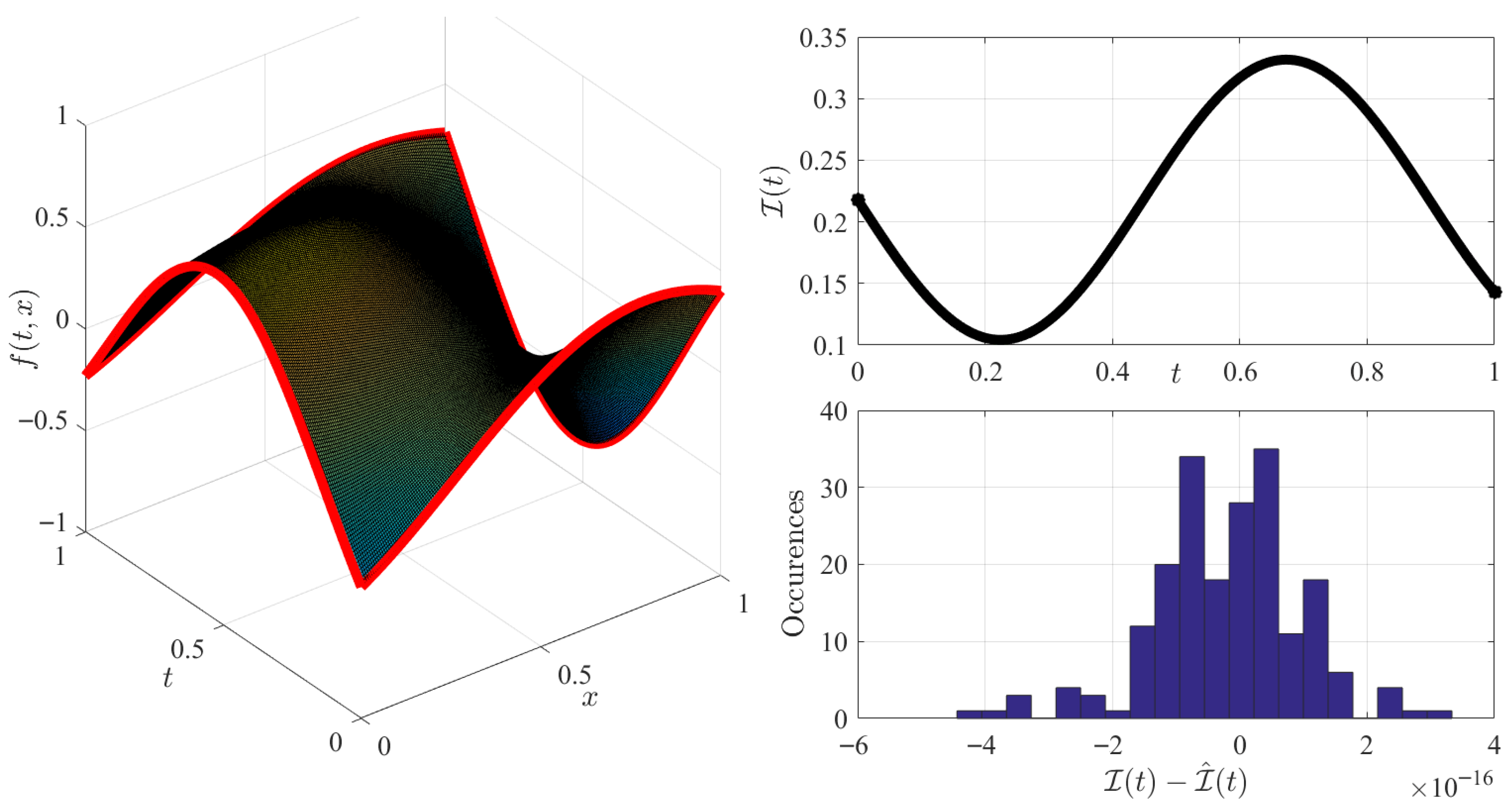
The interpolating surface obtained by Equation (17) using Equation (18) bounds and the time-varying integral given in Equation (19) is shown in the left plot of Figure 3, where the domain has been discretized by 201 × 201 points, uniformly distributed.
The prescribed time-varying integral, J t , p ( t ) of Equation (19), is shown in the left-top plot of Figure 3. Using Simpson’s rule the estimated integral is numerically obtained. The histogram of the differences between prescribed and estimated integrals is shown in the right-bottom plot of Figure 3. The accuracy obtained is close to the machine-error level due to the discretization and the use of the Simpson rule to obtain the estimates.

3.1.2. Functional Interpolation Case

Using the same constraints given in Equations (18) and (19) the functional interpolation case has been tested using the following free functions,
g ( x , t ) = sin ( 9 t ) cos x
whose integral is, x 0 x f g ( x , t ) d x = sin ( 9 t ) sin x f sin x 0 .
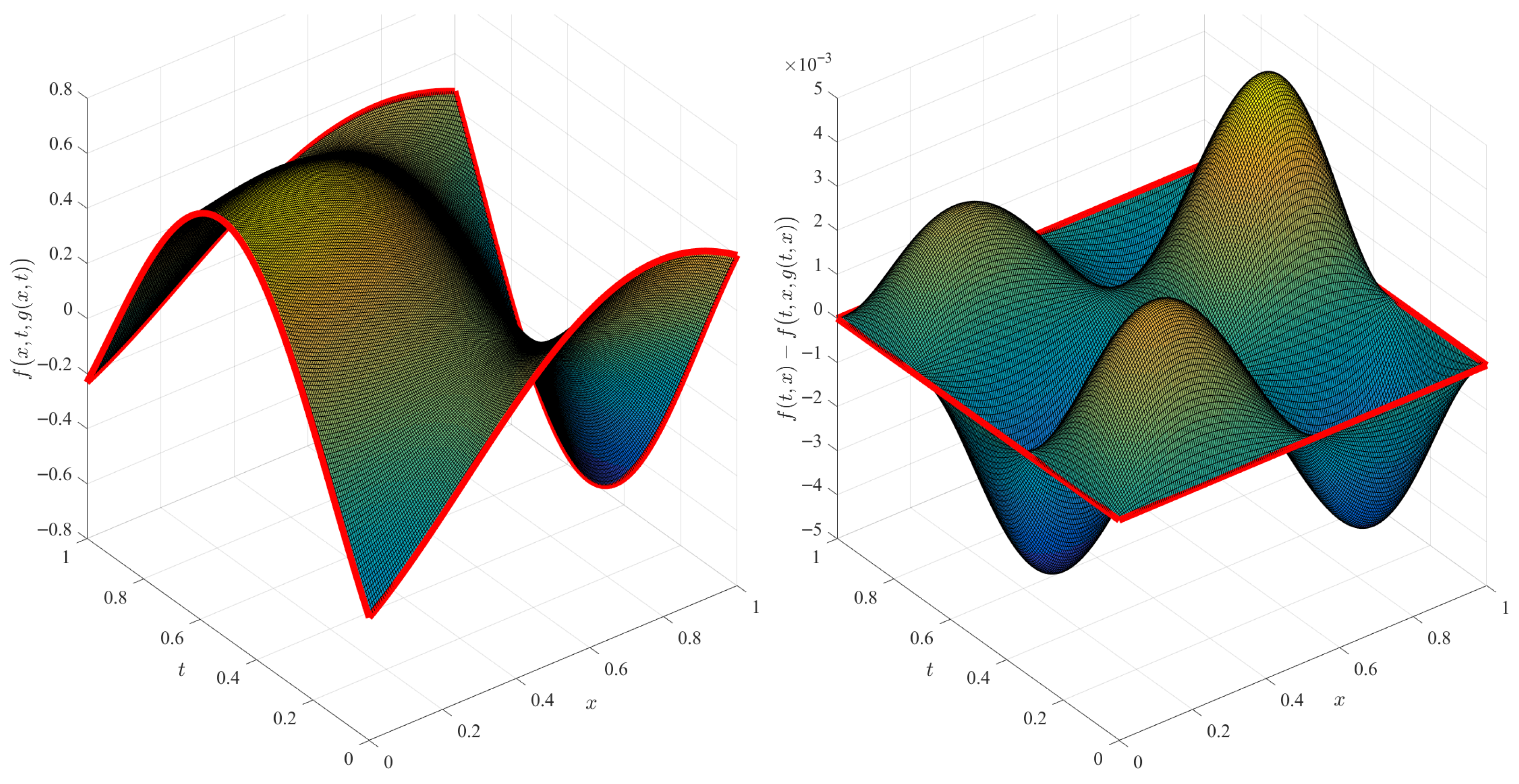
The functional interpolating surface obtained using the same bounds, Equations (18) and (19), and the free function given in Equation (21) is shown in the left plot of Figure 4. The difference between this surface and the one obtained for the interpolation case given in Figure 3 is shown in the left plot of Figure 4.
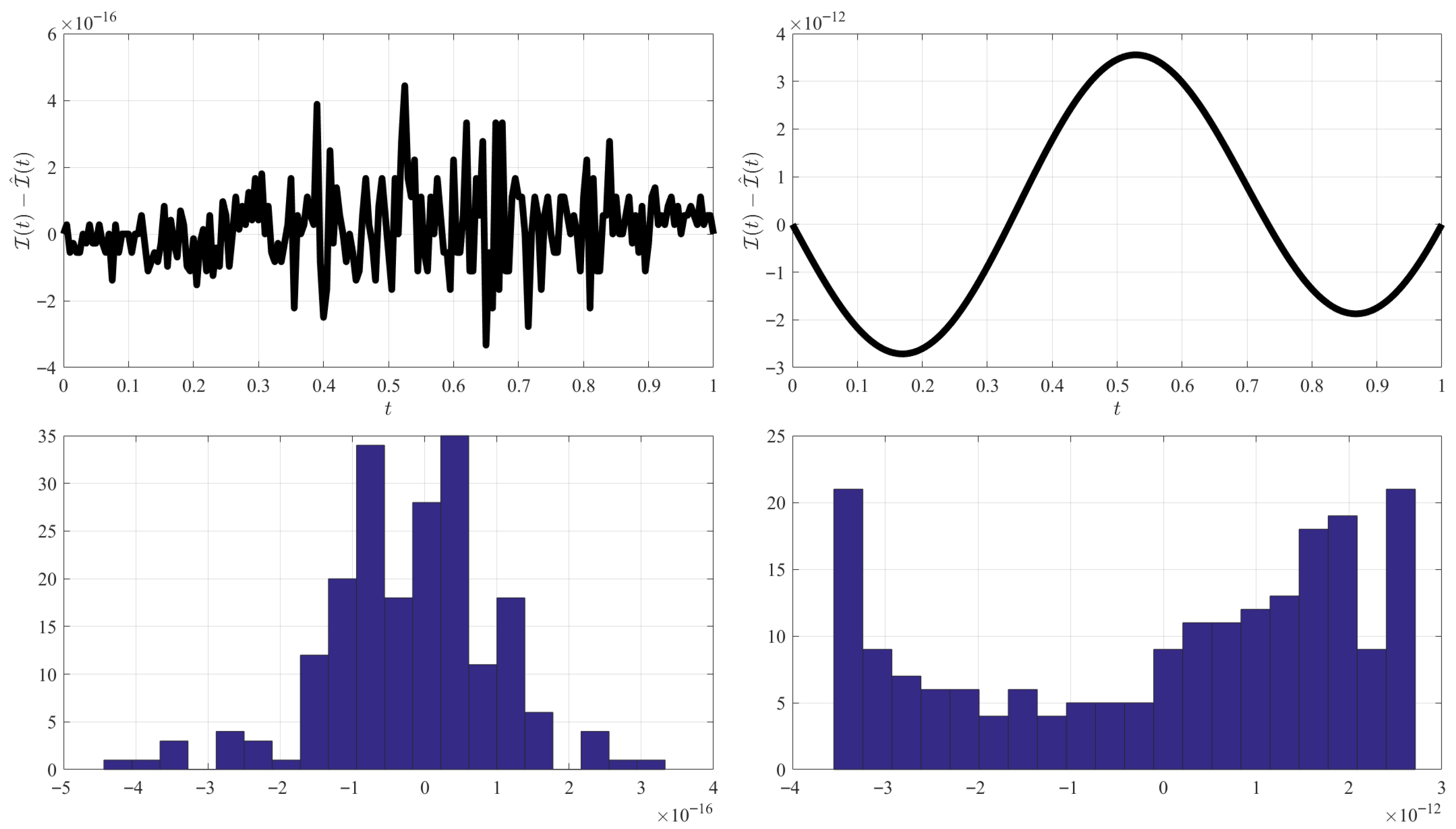
Figure 5 shows, in different ways, the errors obtained for the prescribed integral, Equation (19), in the interpolation case (left plots) and in the functional interpolation case (right plots). The integrals are numerically computed using the Simpson rule, and the errors are quantified to the analytical expression given in Equation (19).
  • Note that, to obtain variations with functional interpolation, that is, using g ( t , x ) 0 , the free function must be linearly independent of the support functions ( 1 , t ) used to derive the constrained functional in t. This means, for instance, that, using g ( t , x ) = ( π t ) cos x , the same surface would have been obtained as using g ( t , x ) = 0 (interpolation case).
  • Note that if the boundary constraints, f ( x 0 , t ) and f ( x f , t ) , and the integral constraint, J t , p ( t ) , are all linear in t, then all b k ( t ) = 0 and, consequently, all η k ( t ) = 0 as well. The resulting interpolating surface will be a linear transformation from the initial f ( x , t 0 ) to the final f ( x , t f ) , and the prescribed integral would play no role.

4. Enforcing Positivity Constraint to Model Probability Density Functions

The functionals associated with continuous integral constraints, as discussed in Section 2.1 and Section 2.2, are designed to satisfy these constraints inherently. The proposed theoretical framework is directly applicable in scenarios where negative values in the resulting solution–whether stemming from a specific choice or the optimal determination of the free function–are physically meaningful. However, this assumption becomes inappropriate when modeling the temporal evolution of a probability density function, as negative values lack physical relevance in classical mechanics. In any case, as discussed in Appendix A, negative probabilities are considered in quantum mechanics, generally interpreted as the cancellation of events.
Although extensive numerical simulations for boundary value problems rarely produce solutions with negative values, this section introduces an alternative approach to address this issue. The proposed method ensures the generation of entirely non-negative least-squares approximated functions, thereby extending the applicability of the theory. Unlike the method described in [23], which employs piecewise linear functions to approximate the solution, the approach presented here focuses on approximating the solution using a single, continuous function. This method not only guarantees the preservation of the integral constraint but also enforces the nonnegativity of the solution.
Let p ( x , t ) represent the time evolution of a probability density function derived from a given free function g ( x , t ) , utilizing the framework outlined in Section 2.1 (for initial value problems) and Section 2.2 (for boundary value problems). Suppose p ( x , t ) < 0 within certain small subdomains of ( x , t ) , which is physically inconsistent for a probability density function. The objective of this section is to construct a least-squares approximation of p ( x , t ) , denoted as p ^ ( x , t ) , that satisfies the nonnegativity constraint, p ^ ( x , t ) 0 , for all ( x , t ) . To achieve this, the modified probability density function is first modeled as
p ^ ( x , t ) = k = 0 n c k ( t ) f k ( x ) ,
where the f k ( x ) are a set of predetermined nonnegative basis functions, such as Bernstein polynomials [24] or Gaussian mixtures [25], and c k ( t ) are unknown nonnegative coefficients. Enforcing these two conditions, p ^ ( x , t ) would never be negative. Coefficients c k ( t ) are estimated using a nonnegative least-squares (NNLS) optimization method [26].
In this study, Bernstein polynomials are selected as the nonnegative basis functions f k ( x ) , as they are well-suited for smooth, bounded approximations and are particularly effective when applied to simpler datasets, while Gaussian mixtures are often preferred for more complex, multimodal datasets (e.g., scenarios with oscillatory behavior) and applications requiring a probabilistic interpretation; they tend to require careful tuning and can face challenges when handling bounded data. Bernstein polynomials, in contrast, provide a robust and straightforward framework for achieving nonnegative approximations in cases involving smooth, single-modal, or well-behaved distributions (Gaussian mixtures are advantageous in modeling highly complex datasets but require parameter tuning and are less effective when the data are bounded or when simplicity is desired).
Bernstein polynomials [24] form a basis for representing continuous functions on the z [ 0 , 1 ] interval. The n + 1 Bernstein polynomials of n degree, f k ( z ) , are the functions,
f k ( z ) = n ! ( n k ) ! k ! z k ( 1 z ) n k , k [ 0 , n ] .
These polynomials satisfy the integral, 0 1 f k ( z ) d z = 1 1 + n . Assuming linear mapping between x (problem variable) and z (Bernstein’s polynomials variable), then
z = x x min x max x min
and mapping the integral in the x variable gives,
x min x max f k ( x ) d x = x max x min 1 + n .

4.1. Non-Negative Least-Squares Methods

A nonnegative least-squares approach solves the problem of minimizing the difference between a given set of observed data (vector b ) and a linear model ( A x ) subject to the constraint that all solution elements must be non-negative,
arg min x A x b 2 2 , subject to x 0 .
This problem can be solved by many approaches (Gradient projection method [27], Multiplicative update method [28], Coordinate descent [29], Interior point method [30], Projected Newton method [31], Alternating direction method of multipliers [32], and the method adopted in this article, the Non-negative quadratic programming). In MATLAB, it can be solved by a single line, x = lsqnonneg(A, b). Alternatively, this problem can be solved by the iterative active set method, as described in [33], consisting of solving the quadratic programming problem,
arg min x 0 1 2 x T Q x + c x where Q = A T A c = A T b .
MATLAB R2024b solves this quadratic programming as, x = quadprog(A’*A, -A’*b, -I, z), where A is the identity matrix of size n + 1 and z a zeros vector of n + 1 elements.

4.2. Univariate Procedure Example

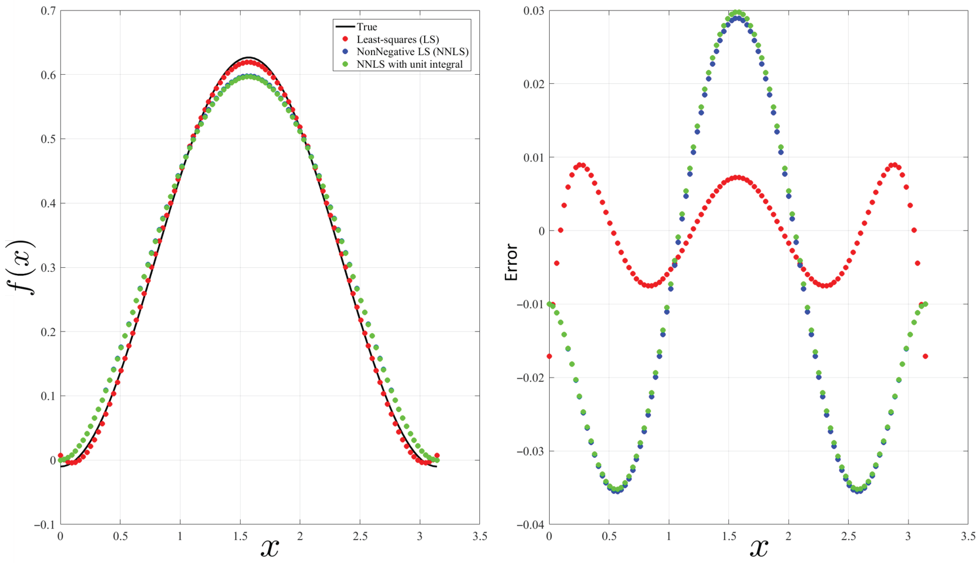
To clarify the procedure, let us consider a straightforward example involving the function f ( x ) = 2 π sin 2 ( x ) 1 100 . This function is depicted in black in Figure 6, and it operates within the specified domain of x [ 0 , π ] . Notably, the function takes on slightly negative values at the domain’s endpoints, specifically at x = 0 and x = π .
In Figure 6, the various markers illustrate different types of approximations applied to the function. Specifically, the red markers represent the least-squares approximation performed using Bernstein polynomials of degree n = 4 (comprising five polynomials) and a domain discretization in 100 points. In contrast, the blue markers (almost coinciding with the green markers) illustrate the nonnegative least-squares approximation using the MATLAB function lsqnonneg, ensuring that the resulting approximations remain nonnegative across the entire domain. Additionally, the green markers indicate the nonnegative least-squares approximation with the unit-integral condition applied, where this condition has been obtained using the method described prior to Section 4. This variant not only maintains the nonnegativity constraints but also ensures that the area under the approximated curve is analytically equal to one, thus adhering to specific normalization requirements. Such distinctions among the different approximation techniques are crucial for understanding how they interact with the characteristics of the original function over the given interval. The same symbols adopted for the left plot are used for the right plot of Figure 6, showing the difference between the exact function, f ( x ) , and the three approximations discussed.
The function f ( x ) is approximated using a selected set of basis functions, specifically Bernstein polynomials of degree n = 4 . Let c k represent the coefficients determined through the Non-Negative Least Squares (NNLS) approximation. To ensure that the resulting approximation satisfies a unit-integral condition, these coefficients must undergo a rescaling process. This rescaling leverages both the integral property of Bernstein polynomials over their entire domain and the linear mapping function defined in Equation (22). The rescaled coefficients, denoted by c ^ k , are derived from the original coefficients c k using the relationship,
c ^ k = c k n + 1 x max x min i = 0 n c i
Incorporating these modified coefficients results in an approximated function expressed as,
p ^ ( x , t ) = k = 0 n c ^ k ( t ) f k ( x )
This formulation not only enforces the unit-integral condition analytically but also guarantees that the resulting function maintains strict positivity across its entire domain.
The implementation of the proposed method to a given probability density function, f ( t , x ) , which is derived from an optimization process, is specifically designed to address cases where the function f ( t , x ) exhibits negative values. The described mitigation method can be applied globally across the entire domain using a two-dimensional least-squares optimization process. Alternatively, as demonstrated in the preceding example, the approach can be applied locally by discretizing the time variable, t, into distinct time steps, t k [ t min , t max ] . For each time step, the method is then employed on the corresponding univariate function f ( t k , x ) , which approximates the probability density function evaluated at the specific time t k .

5. Discussion

This document presents an extension to the Theory of Functional Connections (TFC) focusing on functionals that involve continuous integral constraints. TFC was initially developed to address functional interpolation problems involving points, integer and fractional derivatives and integrals, limits, and any linear combination of these constraints, applicable to both univariate and multivariate cases. Unlike previous applications of TFC, for the first time, this study directly applies it to continuous constraints. The paper explores how to derive functionals that meet continuous integral constraints, which are essential for maintaining physical laws like conservation of energy and probability in various applications, especially those involving stochastic differential equations.
Specifically, we explore constraints of the form x 0 x f f ( x , t ) d x = J ( t ) , where J ( t ) is either a predefined function or an unknown function that must be determined as part of an optimization problem. This expansion opens the door to addressing problems with dynamic conditions over time, which are critical in fields ranging from control theory to physics. In particular, we explore the case of time-invariant integral constraints, where J ( t ) = is constant, for initial and boundary value problems. Such constraints are critical in maintaining physical laws, such as the conservation of mass, energy, or probability in dynamic systems.
The proposed methodology has been generalized to accommodate time-varying continuous integral constraints. These integrals can either be prescribed explicitly in advance or treated as unknown functions to be determined through optimization techniques. The approach has broad applicability across a wide range of disciplines where the integral of some function plays a critical role, including fluid dynamics, electromagnetism, and statistical mechanics. To illustrate the effectiveness of the proposed method, a numerical example is presented, demonstrating the operation of a prescribed time-varying integral functional.
The work also tackles the challenge of enforcing positivity constraints in modeling probability density functions, which is crucial for physical validity. Unfortunately, the proposed approach to obtaining a continuous integral constraint does not analytically guarantee the positivity constraint, which remains a challenge within the TFC framework. Although negative values are rarely observed in extensive numerical tests when using the proposed approach, a mitigation method has been developed to address this issue when it arises. To address the positivity constraint, a least-squares algorithm is proposed that can be applied when the optimal PDF evolution assumes small negative values. This approach mitigates the problem by providing an approximate continuous PDF evolution based on a nonnegative least-squares method, using Bernstein’s polynomials, and rescaling the least-squares coefficients.
This study contributes to the ongoing development of TFC by offering a new method to handle more complex continuous constraints, expanding its applicability to problems previously out of reach due to their dynamic or non-standard nature. The theoretical developments presented here, supported by numerical results, open up new possibilities for both classical and quantum systems governed by conservation laws, with far-reaching implications for future research and application.
Finally, this study includes a brief appendix note on the concept of negative probabilities within the context of quantum mechanics.

Funding

This research received no external funding.

Conflicts of Interest

The author declares no conflicts of interest.

Abbreviations

The following abbreviations are used in this manuscript:
TFCTheory of Functional Connections
DEDifferential Equation

Appendix A. Note on Negative Probability

Paul Dirac introduced in 1941 both the concepts of negative energies and negative probabilities [34]. Later, R. Feynman [35] argued how negative probabilities as well as probabilities above unity possibly could be useful in probability calculations. Negative probabilities expand the notion of probability by allowing for the cancelation of events, introducing a new level of flexibility in probabilistic modeling. In classical probabilities, when an event has occurred, it has happened, and there is nothing you can change about it. In negative probabilities, events can be canceled. There are positive events and negative (anti) events. However, negative probabilities must always be combined with positive ones to give an ordinary probability.
This perspective emphasizes that while probabilities of verifiable events cannot be negative, intermediate states and theoretical constructs may yield negative probabilities that provide insights into the underlying mechanics of a system.
In quantum mechanics, negative probabilities have been used to explain phenomena that cannot be observed directly. For instance, in the context of the Wigner function, which is used to describe the quantum state of a system, negative probabilities can arise [36]. These negative values do not correspond to actual probabilities of observable events but serve as tools in the mathematical modeling of these systems. They can help in understanding the relationships between unobservable latent variables and their implications for measurable quantities.
Despite its mathematical utility, the interpretation of negative probabilities remains complex and often controversial. Many physicists and mathematicians argue that while negative probabilities can facilitate calculations and simulations in specific contexts [37], they also introduce philosophical questions regarding the nature of probability itself. The challenge lies in reconciling negative probabilities with conventional views on measurement, reality, and observable phenomena.

References

  1. Mortari, D. The Theory of Connections: Connecting Points. Mathematics 2017, 5, 57. [Google Scholar] [CrossRef]
  2. Mortari, D. Least-Squares Solution of Linear Differential Equations. Mathematics 2017, 5, 48. [Google Scholar] [CrossRef]
  3. Leake, C.D. The Multivariate Theory of Functional Connections: An n-Dimensional Constraint Embedding Technique Applied to Partial Differential Equations. Ph.D. Thesis, Texas A&M University, College Station, TX, USA, 2021. [Google Scholar]
  4. Johnston, H.R. The Theory of Functional Connections: A Journey from Theory to Application. Ph.D. Thesis, Texas A&M University, College Station, TX, USA, 2021. [Google Scholar]
  5. Leake, C.; Johnston, H.; Mortari, D. The Theory of Functional Connections: A Functional Interpolation Framework with Applications; Lulu: Morrisville, NC, USA, 2022. [Google Scholar]
  6. Mortari, D. Theory of Functional Connections Subject to Shear-Type and Mixed Derivatives. Mathematics 2022, 10, 4692. [Google Scholar] [CrossRef]
  7. Mortari, D.; Garrappa, R.; Nicolò, L. Theory of Functional Connections Extended to Fractional Operators. Mathematics 2023, 11, 1721. [Google Scholar] [CrossRef]
  8. Mortari, D. Representation of Fractional Operators using the Theory of Functional Connections. Mathematics 2023, 11, 4772. [Google Scholar] [CrossRef]
  9. Mortari, D. Using the Theory of Functional Connections to Solve Boundary Value Geodesic Problems. Math. Comput. Appl. 2022, 27, 64. [Google Scholar] [CrossRef]
  10. Wang, Y.; Topputo, F. A TFC-based homotopy continuation algorithm with application to dynamics and control problems. J. Comput. Appl. Math. 2022, 401, 113777. [Google Scholar] [CrossRef]
  11. D’Ambrosio, A.; Schiassi, E.; Johnston, H.R.; Curti, F.; Mortari, D.; Furfaro, R. Time-energy optimal landing on planetary bodies via theory of functional connections. Adv. Space Res. 2022, 69, 4198–4220. [Google Scholar] [CrossRef]
  12. Schiassi, E.; D’Ambrosio, A.; Furfaro, R. An Overview of X-TFC Applications for Aerospace Optimal Control Problems. In The Use of Artificial Intelligence for Space Applications. Workshop at the 2022 International Conference on Applied Intelligence and Informatics; Springer Nature: Berlin/Heidelberg, Germany, 2023; Volume 1088, p. 199. [Google Scholar]
  13. De Florio, M.; Schiassi, E.; Furfaro, R. Physics-informed neural networks and functional interpolation for stiff chemical kinetics. Chaos Interdiscip. J. Nonlinear Sci. 2022, 32, 063107. [Google Scholar] [CrossRef] [PubMed]
  14. Schiassi, E.; De Florio, M.; D’Ambrosio, A.; Mortari, D.; Furfaro, R. Physics-informed neural networks and functional interpolation for data-driven parameters discovery of epidemiological compartmental models. Mathematics 2021, 9, 2069. [Google Scholar] [CrossRef]
  15. Mai, T.; Mortari, D. Theory of Functional Connections Applied to Quadratic and Nonlinear Programming under Equality Constraints. J. Comput. Appl. Math. 2022, 406, 113912. [Google Scholar] [CrossRef]
  16. Yassopoulos, C.; Reddy, J.; Mortari, D. Analysis of Timoshenko-Ehrenfest Beam Problems using the Theory of Functional Connections. J. Eng. Anal. Bound. Elem. 2021, 132, 271–280. [Google Scholar] [CrossRef]
  17. Yassopoulos, C.; Reddy, J.; Mortari, D. Analysis of nonlinear Timoshenko–Ehrenfest Beam Problems with Von Kármán Nonlinearity using the Theory of Functional Connections. Math. Comput. Simul. 2023, 205, 709–744. [Google Scholar] [CrossRef]
  18. Leake, C.; Mortari, D. Deep theory of functional connections: A new method for estimating the solutions of partial differential equations. Mach. Learn. Knowl. Extr. 2020, 2, 37–55. [Google Scholar] [CrossRef] [PubMed]
  19. Schiassi, E.; Furfaro, R.; Leake, C.D.; Florio, M.D.; Johnston, H.R.; Mortari, D. Extreme Theory of Functional Connections: A Fast Physics-Informed Neural Network Method for Solving Ordinary and Partial Differential Equations. Neurocomputing 2021, 457, 334–356. [Google Scholar] [CrossRef]
  20. Raissi, M.; Perdikaris, P.; Karniadakis, G.E. Physics-informed neural networks: A deep learning framework for solving forward and inverse problems involving nonlinear partial differential equations. J. Comput. Phys. 2019, 378, 686–707. [Google Scholar] [CrossRef]
  21. Wikipedia. Physics-Informed Neural Networks—Wikipedia, The Free Encyclopedia. 2024. Available online: http://en.wikipedia.org/w/index.php?title=Physics-informed%20neural%20networks&oldid=1251520404 (accessed on 26 October 2024).
  22. Mortari, D.; Johnston, H.R.; Smith, L. High Accuracy Least-squares Solutions of Nonlinear Differential Equations. J. Comput. Appl. Math. 2019, 352, 293–307. [Google Scholar] [CrossRef]
  23. Ding, J.; Eifler, L.; Rhee, N. Integral and nonnegativity preserving approximations of functions. J. Math. Anal. Appl. 2007, 325, 889. [Google Scholar] [CrossRef]
  24. Lorentz, G.G. Bernstein Polynomials; American Mathematical Society: Providence, RI, USA, 2012. [Google Scholar]
  25. Reynolds, D.A. Gaussian mixture models. Encycl. Biom. 2009, 741, 827–832. [Google Scholar]
  26. Wikipedia. Non-Negative Least Squares. 2004. Available online: https://en.wikipedia.org/wiki/Non-negative_least_squares (accessed on 24 November 2024).
  27. Kim, D.; Sra, S.; Dhillon, I.S. Fast Projection-Based Methods for the Least Squares Nonnegative Matrix Approximation Problem. Stat. Anal. Data Min. 2008, 1, 38–51. [Google Scholar] [CrossRef]
  28. Zhao, R.; Tan, V.Y. A unified convergence analysis of the multiplicative update algorithm for regularized nonnegative matrix factorization. IEEE Trans. Signal Process. 2017, 66, 129–138. [Google Scholar] [CrossRef]
  29. Hsieh, C.J.; Dhillon, I.S. Fast coordinate descent methods with variable selection for non-negative matrix factorization. In Proceedings of the 17th ACM SIGKDD International Conference on Knowledge Discovery and Data Mining, San Diego, CA, USA, 21–24 August 2011; pp. 1064–1072. [Google Scholar]
  30. Kim, S.J.; Koh, K.; Lustig, M.; Boyd, S.; Gorinevsky, D. An interior-point method for large-scale 1-regularized least squares. IEEE J. Sel. Top. Signal Process. 2007, 1, 606–617. [Google Scholar] [CrossRef]
  31. Gong, P.; Zhang, C. Efficient nonnegative matrix factorization via projected Newton method. Pattern Recognit. 2012, 45, 3557–3565. [Google Scholar] [CrossRef]
  32. Zdunek, R. Alternating direction method for approximating smooth feature vectors in nonnegative matrix factorization. In Proceedings of the 2014 IEEE International Workshop on Machine Learning for Signal Processing (MLSP), Reims, France, 21–24 September 2014; IEEE: Piscataway, NJ, USA, 2014; pp. 1–6. [Google Scholar]
  33. Lawson, C.L.; Hanson, R.J. Solving Least Squares Problems; SIAM: Bangkok, Thailand, 1995; Chapter 23; p. 161. [Google Scholar]
  34. Dirac, P.A.M. The physical interpretation of the quantum dynamics. Proc. R. Soc. Lond. Ser. A Contain. Pap. Math. Phys. Character 1927, 113, 621–641. [Google Scholar]
  35. Feynman, R.P. Negative Probability. 1984. Available online: https://cds.cern.ch/record/154856/files/pre-27827.pdf (accessed on 24 November 2024).
  36. Weinbub, J.; Ferry, D. Recent advances in Wigner function approaches. Appl. Phys. Rev. 2018, 5, 041104. [Google Scholar] [CrossRef]
  37. Blass, A.; Gurevich, Y. Negative probabilities: What they are and what they are for. arXiv 2020, arXiv:2009.10552. [Google Scholar]
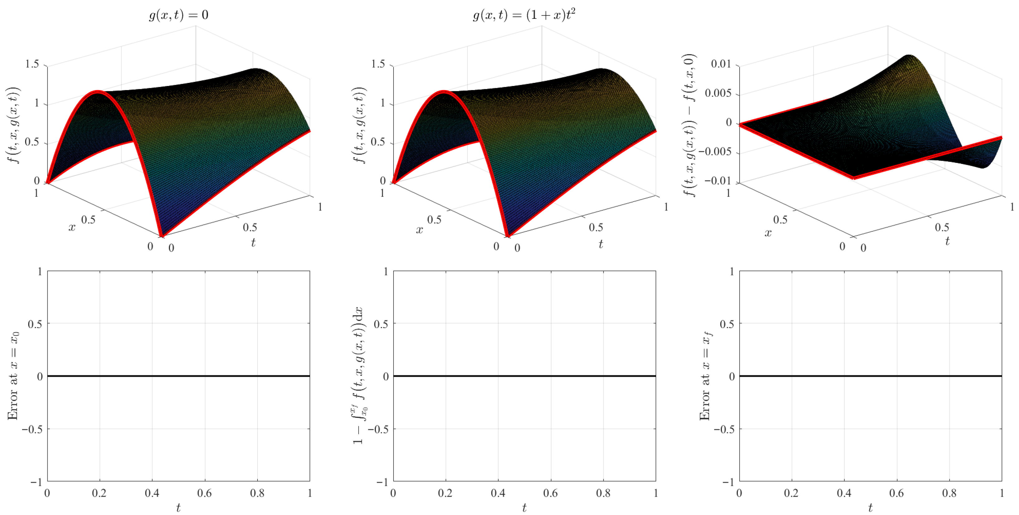
Figure 1. Numerical validation of integral invariant functionals for IVP problems.
Mca 30 00105 g001
Figure 2. Numerical validation of integral invariant functionals for BVP problems.
Mca 30 00105 g002
Figure 3. Time-varying integral surface obtained using g ( x , t ) = 0 . Boundaries are shown in red.
Mca 30 00105 g003
Figure 4. Time-varying integral surface using g ( x , t ) = sin ( 9 t ) cos x (left) and the surface difference for the interpolation case, using g ( x , t ) = 0 (right).
Mca 30 00105 g004
Figure 5. Interpolation ((left), g ( x , t ) = 0 ) and functional interpolation ((right), g ( x , t ) = sin ( 9 t ) cos x ) integral errors (top) and integral errors histograms (bottom).
Mca 30 00105 g005
Figure 6. Example of fitting function f ( x ) by least-squares (red), nonnegative least-squares (blue), and nonnegative least-squares with unit-intergral (green).
Mca 30 00105 g006
Disclaimer/Publisher’s Note: The statements, opinions and data contained in all publications are solely those of the individual author(s) and contributor(s) and not of MDPI and/or the editor(s). MDPI and/or the editor(s) disclaim responsibility for any injury to people or property resulting from any ideas, methods, instructions or products referred to in the content.