Statistical Modeling of Reliable Intervals for Solutions to Linear Transfer Problems Under Boundary Experimental Data

Abstract

A methodology for the statistical modeling of boundary value problems of mathematical physics for parabolic equations used to describe transport processes in a layer with incomplete data at the boundary of a body has been developed and presented. The boundary value problem is formulated for the case of a non-zero initial condition, the presence of a stable source at one boundary of the body (classical boundary condition), and a sample of experimental data for the desired function at the other boundary (statistical boundary condition). A linear regression model obtained from experimental data by the least squares method is used as a boundary condition. The article defines two-sided statistical estimates of the solution of the boundary value problem through linear regression coefficients, analyzes the mathematical model taking into account the influence of the sample size and covariance, determines the reliable intervals for linear regression and the desired function depending on the given level of reliability. The influence of the experimental data statistical characteristics on the desired function at the lower layer’s boundary for different types of samples in the case of large or small-time intervals is studied. The two-sided critical domain is obtained and analyzed on the basis of Fisher’s criterion. The influence of the reliability level on the reliable intervals, the solution to the parabolic boundary value problem, and the width of the bilateral critical domain constructed for the solution is analyzed.

1. Introduction

Various tasks in engineering, ecology, biology, pharmacology, and other technical and technological research require the further development of approaches and methods for the mathematical description of non-equilibrium processes of a different physical nature [1]. The relevance of the above problems is caused by the need to develop effective methods and estimates for predicting the distribution of man-made pollution, assessing the quality of drinking water and improving its treatment on an industrial scale, determining the effect of diffusion of drugs into tissue, diffusion of aggressive substances when assessing the reliability and durability of structural elements and components to prevent the destruction of the relevant materials, etc. Therefore, statistical modeling methods that combine classical approaches to mathematical modeling and methods of mathematical statistics are relevant. These studies enable us to obtain a reliable forecast of the processes taking place in environmental objects, industrial equipment units, the human body, etc., and to take the necessary measures in time to prevent their negative development. The main approaches and methods of statistical modeling have been developing quite rapidly over the past few decades [2,3].

These methods are widely used in environmental problems. The complexity of the study is explained by the multiphase behavior of the diffusion process. Over recent decades, researchers have developed various statistical models of multiphase flow, mass transfer, and solute transport to simulate the distribution of groundwater contamination [4,5], to explore the concepts of electrochemical nucleation, and in [6,7] to analyze meteorological fields obtained to reflect the characteristics of air pollution. Statistical modeling methods are actively used in biology and medicine. In [8], a deterministic and statistical model describing synaptic communication in a biological molecular communication system was proposed and formulated for the diffusion equation in terms of a hypergeometric distribution. Özdural et al. [9] presented a mathematical statistical model based on nonequilibrium conditions that describes the dynamic adsorption of proteins. A data-driven methodology for economical modeling and the analysis of dynamic cerebral autoregulation of arterial blood pressure, cerebral blood flow velocity, and their time derivatives was developed [10]. The dynamics of diffusion processes were analyzed by examining the eigenvalues of the Markov random walk matrix in the data set. Blood propagation, blood flow dynamics, and diffusion were modeled in [11] using the Monte Carlo method and the laminar Navier–Stokes equation. Computational statistical models help to eliminate the risks of excessive blood heating and improve the design of blood flow devices. Models of the diffusion release of drugs from hydrogel ophthalmic lenses were analyzed using probabilistic modeling methods in [12].

The statistical modeling technique has shown particular efficiency in engineering problems. The aim of paper [13] was to model heat and mass transfer in electronics problems, whose mathematical models are based on the perturbed circuit equation. Using the precise numerical statistical modeling of flow and transfer, Gouze et al. [14] studied the increase in the scale of passive dissolved matter transfer in a carbonate rock sample characterized by microporous areas. Statistical modeling was used in [15] to study the transfer of dissolved oxygen with a high Schmidt number from oscillating turbulent flows to a permeable layer of microbial sediment. The mathematical model of the kinetics of neutral particles diluted in a gas or plasma and reacting with a catalytic surface is formulated as a boundary value problem for the reaction–diffusion equation. However, this approximation does not always adequately reflect the transfer process. As an alternative, Longo et al. [16] used Monte Carlo simulation, taking into account the problem of statistical error. The aim of the study [17] is to develop probabilistic analytical models for predicting the characteristics of concrete in terms of chloride penetration. Gusev and Nikolaev [18] proposed a method for assessing the thermal state of insulating cellular panels, which is described by a boundary value problem for a parabolic equation with a discontinuous diffusion coefficient and boundary conditions of the third kind. The problem is solved by means of a probabilistic representation of the functional expectation of the diffusion process corresponding to the boundary value problem. The possibility of the non-invasive determinationof the diffusion approximation parameters in the radiation transfer theory under the condition of fixing the input radiation power was researched by numerical and statistical modeling in [19]. De Lemos and Mesquita [20] presented a numerical simulation of the combustion of an air/methane mixture in porous materials using a model that accounts for intra-pore levels of turbulent kinetic energy. Statistical tests and corresponding mathematical modeling were used in [21] to determine the effect of temperature, moisture content, density, and porosity of the material on the effective moisture diffusion coefficient during the convective drying of celery root. A statistical approach for modeling small molecules at non-zero concentrations in microporous materials was developed in [22].

It should be noted separately that statistical modeling in recent years has received its further development on the basis of approaches based on various nonlinear regression models [23]. The study [24] proposes a new method for calculating nonlinear heat conduction processes under Robin boundary conditions. The article [25] develops and implements an effective numerical scheme for studying solutions to the nonlinear diffusion mass transfer problem.

In view of the need to solve the problems mentioned above and a number of other similar problems, a certain mathematical apparatus for statistical modeling of reaction–diffusion problems has been developed. A systematic presentation of methods and approaches to statistical modeling of random diffusion fluxes of impurity particles in a two-phase stratified strip with a stochastic arrangement of phases and random thickness of inclusion layers is given in [26]. Similar diffusion models are important in the design of composite layered materials [27], the study of filter throughput properties [28], the prediction of the spread of pollutants in the environment, etc. The calculation formulas for the diffusion flux averaged over an ensemble of phase configurations and over the thickness of the inclusion were obtained.

The analysis of the problem has shown that it is not always possible to correctly impose boundary conditions on the boundaries based on physical considerations, even in a fairly general form. This is due to the complexity and insufficiency of the relevant research, and therefore, the analysis and necessary generalizations are lacking. Following the above, a mathematical model of the transfer process in the layer under the condition of the given experimental data on a part of the layer boundary was developed and studied in [29]. From the experimental data, a boundary condition is constructed, the corresponding mixed problem is formulated and solved, the influence of the statistical characteristics of the sample of experimental data on the solution is analyzed, and a two-sided statistical estimate of the solution is determined. The reliable intervals for the coefficients of the regression equation and the corresponding reliable intervals for the required function are established in the case of different samples in terms of size and variance.

This paper considers a parabolic boundary value problem that describes the processes of heat, mass, charge, etc., transfer in a layer when experimental data on the required function are available at one of the boundaries under a non-zero initial condition.The main focus of the research in this article is to expand and generalize the range of possible statistical modeling approaches to studying the linear transport models, presented in [26,27,28,29]. In particular, developing the ideas and approaches of the paper [29], we present an effective method for establishing reliable intervals for solutions of parabolic differential equations with experimental data at the boundary of the body and analyze the influence of the reliability level on the width of reliable intervals. Developing and generalizing the methodology of the above-mentioned papers, a two-sided critical domain for the solution is constructed. The aim of the article is to conduct a numerical analysis of the solution of the boundary value problem depending on the statistical characteristics of the sample. The article also investigates the influence of the reliablelevel on the reliable intervals for the linear regression and for the solution of the parabolic boundary value problem.

2. Formulation of a Boundary Value Problem for a Parabolic Equation in a Layer with Experimental Data at the Boundary

In the layer with the thickness $z_0$, the process described by the function $u(\tau ,z)$, takes place, being a solution of the second-order partial differential equation [30]

$${\displaystyle \frac{\mathsf{\partial }u(\tau ,z)}{\mathsf{\partial }\tau }}=A{\displaystyle \frac{{\mathsf{\partial }}^{2}u(\tau ,z)}{\mathsf{\partial }{z}^2}},$$

(1)

where $A$ is a constant coefficient, $\tau$ is time, and $z$ is a spatial coordinate.

We assume that at the initial moment the function $u(\tau ,z)$

$${\left.u(\tau ,z)\right|}_{\tau =0}=u_0\equiv const,$$

(2)

and at $\tau >0$ the upper surface of the layer is subjected to a stable source

$${\left.u(\tau ,z)\right|}_{z=0}=u_{*}\equiv const.$$

(3)

At the lower boundary of the layer, the values of the function $u(\tau ,z)$ were obtained experimentally at $n$ time points (

Table 1. Experimental data at the lower boundary of the layer.

$\tau$	${\tau }_1$	${\tau }_2$	…	${\tau }_i$	…	${\tau }_n$
${\left.u(\tau )\right|}_{z_0}$	$u_{z_0}({\tau }_1)$	$u_{z_0}({\tau }_2)$	…	$u_{z_0}({\tau }_i)$	…	$u_{z_0}({\tau }_n)$

).

Then a linear regression model is built [31,32], searching for its coefficients using the least squares method [33]

$$f(\tau )=a_1\tau +a_0.$$

(4)

The coefficients $a_1$ and $a_0$ are calculated using the following formulas

$$a_1={\displaystyle \frac{n{\displaystyle \sum _{i=1}^n{\tau }_i{u}_{z_{0}i}}-\left({\displaystyle \sum _{i=1}^n{\tau }_i}\right)\left({\displaystyle \sum _{i=1}^n{u}_{z_{0}i}}\right)}{n\left({\displaystyle \sum _{i=1}^n{\tau }_i^2}\right)-{\left({\displaystyle \sum _{i=1}^n{\tau }_i}\right)}^2}},$$

(5)

$$a_0={\displaystyle \frac{\left({\displaystyle \sum _{i=1}^n{\tau }_i^2}\right)\left({\displaystyle \sum _{i=1}^n{u}_{z_{0}i}}\right)-\left({\displaystyle \sum _{i=1}^n{\tau }_i}\right)\left({\displaystyle \sum _{i=1}^n{\tau }_i{u}_{z_{0}i}}\right)}{n\left({\displaystyle \sum _{i=1}^n{\tau }_i^2}\right)-{\left({\displaystyle \sum _{i=1}^n{\tau }_i}\right)}^2}},$$

(6)

where $u_{z_{0}i}=u_{z_0}({\tau }_i)$. As a result, the boundary condition at $z=z_0$ will take the form

$${\left.u(\tau ,z)\right|}_{z=z_0}=f(\tau ).$$

(7)

3. Solving a Parabolic Boundary Value Problem Under the Condition of Linear Regression on the Layer Boundary

To solve the problem (1)–(3), (7) by way of substitution

$$v(\tau ,z)=u(\tau ,z)-u_{*}\left(1-{\displaystyle \frac{z}{z_0}}\right)-f(\tau ){\displaystyle \frac{z}{z_0}}$$

(8)

one can reduce it to a problem with zero boundary conditions with respect to the function $v(\tau ,z)$

$${\displaystyle \frac{\mathsf{\partial }v(\tau ,z)}{\mathsf{\partial }\tau }}+{\displaystyle \frac{\mathsf{\partial }f(\tau )}{\mathsf{\partial }\tau }}{\displaystyle \frac{z}{z_0}}=A{\displaystyle \frac{{\mathsf{\partial }}^{2}v(\tau ,z)}{\mathsf{\partial }{z}^2}}.$$

(9)

The required function $v(\tau ,z)$ satisfies the initial condition

$${\left.v(\tau ,z)\right|}_{\tau =0}=u_0-u_{*}\left(1-{\displaystyle \frac{z}{z_0}}\right)-{\left.f(\tau )\right|}_{\tau =0}{\displaystyle \frac{z}{z_0}}$$

(10)

and zero boundary conditions

$${\left.v(\tau ,z)\right|}_{z=0}={\left.v(\tau ,z)\right|}_{z=z_0}=0.$$

(11)

Applying to the boundary value problem (9)–(11) the finite integral Fourier sin-transform [34] ($z\to y_m=$$m\pi /z_0$, $v(\tau ,z)\to \tilde{v}(\tau ,y_m)$), the next problem is obtained in images

$${\displaystyle \frac{d\tilde{v}(\tau ,y_m)}{d\tau }}+A{y}_m^2\tilde{v}(\tau ,y_m)={\displaystyle \frac{df(\tau )}{d\tau }}{\displaystyle \frac{{(-1)}^m}{y_m}},$$

(12)

$${\left.\tilde{v}(\tau ,z)\right|}_{\tau =0}={\displaystyle \frac{1}{y_m}}\left(u_0-u_{*}+{(-1)}^{m+1}\left(u_0-{\left.f(\tau )\right|}_{\tau =0}\right)\right).$$

(13)

The solution to problems (12) and (13) is the following expression [35]

$$\begin{array}{l}\tilde{v}(\tau ,y_m)={\displaystyle \frac{{(-1)}^m}{y_m}}f(\tau )+e^{-A{y}_m^2\tau }\left\{\left({\displaystyle \frac{1}{y_m}}\left(u_0-u_{*}+{(-1)}^{m+1}{u}_0\right)\right)\right.\\ \left.+{\displaystyle \frac{{(-1)}^m}{y_m}}A{y}_m^2{\left.{\displaystyle \int f(\tau )e^{A{y}_m^2\tau }d\tau }\right|}_{\tau =0}-{\displaystyle \frac{{(-1)}^m}{y_m}}A{y}_m^2{\displaystyle \int f(\tau )e^{A{y}_m^2\tau }d\tau }\right\}\end{array}.$$

(14)

After the Fourier sin-transform [36] is applied to the relationship (14), one can obtain

$$\begin{array}{l}v(\tau ,z)={\displaystyle \frac{2}{z_0}}{\displaystyle \sum _{m=1}^{\infty }\frac{{(-1)}^m}{y_m}f(\tau )}\sin (y_{m}z)+{\displaystyle \frac{2}{z_0}}{\displaystyle \sum _{n=1}^{\infty }{e}^{-A{y}_m^2\tau }\left(\frac{1}{y_m}\left(u_0-u_{*}+{(-1)}^{m+1}{u}_0\right)\right)\sin (y_{m}z)}\\ +{\displaystyle \frac{2}{z_0}}{\displaystyle \sum _{m=1}^{\infty }{e}^{-A{y}_m^2\tau }\left(\frac{{(-1)}^m}{y_m}A{y}_m^2{\left.{\displaystyle \int f(\tau )e^{A{y}_m^2\tau }d\tau }\right|}_{\tau =0}-\frac{{(-1)}^m}{y_m}A{y}_m^2{\displaystyle \int f(\tau )e^{A{y}_m^{2}t}\tau d\tau }\right)\sin (y_{m}z)}\end{array}.$$

Taking into account (8), the solution to the problem (1)–(3), (7) is obtained in the form

$$\begin{gathered} u(\tau ,z)=u_{*}\left(1-{\displaystyle \frac{z}{z_0}}\right)+f(\tau ){\displaystyle \frac{z}{z_0}}+{\displaystyle \frac{2}{z_0}}{\displaystyle \sum _{m=1}^{\infty }\left\{\frac{{(-1)}^m}{y_m}\right.f(\tau )+}{\displaystyle \frac{e^{-A{y}_m^2\tau }}{y_m}}\left(u_0-u_{*}+{(-1)}^{m+1}{u}_0\right. \\ \left.\left.+{(-1)}^{m}A{y}_m^2{\left.{\displaystyle \int f(\tau )e^{A{y}_m^2\tau }d\tau }\right|}_{\tau =0}-{(-1)}^{m}A{y}_m^2{\displaystyle \int f(\tau )e^{A{y}_m^2\tau }d\tau }\right)\right\}\sin (y_{m}z) \end{gathered}$$

(15)

Formula (15) can be specified taking into account that it is a linear regression, i.e., Formula (4) is valid. Then

$$\begin{gathered} {(-1)}^m{y}_m{e}^{-A{y}_m^2\tau }{\displaystyle \int f(\tau )}\hspace{0.17em}\hspace{0.17em}{e}^{A{y}_m^2\tau }\hspace{0.17em}d\tau ={\displaystyle \frac{{(-1)}^m}{A{y}_m}}\left[a_1\tau +a_0-{\displaystyle \frac{a_1}{A{y}_m^2}}\right]; \\ {\left.{(-1)}^m{y}_m{\displaystyle \int f(\tau )}\hspace{0.17em}\hspace{0.17em}{e}^{A{y}_m^2\tau }\hspace{0.17em}d\tau \right|}_{\tau =0}={\displaystyle \frac{{(-1)}^m}{A{y}_m}}\left[a_0-{\displaystyle \frac{a_1}{A{y}_m^2}}\right] \end{gathered}$$

and, accordingly, the solution becomes

$$\begin{gathered} u(\tau ,z)=u_{*}\left(1-{\displaystyle \frac{z}{z_0}}\right)+(a_1\tau +a_0){\displaystyle \frac{z}{z_0}}+{\displaystyle \frac{2}{z_0}}{\displaystyle \sum _{m=1}^{\infty }\left\{a_1\frac{{(-1)}^m}{A{y}_m^3}\right.} \\ \left.+{\displaystyle \frac{e^{-A{y}_m^2\tau }}{y_m}}\left[u_0-u_{*}+{(-1)}^{m+1}{u}_0+{(-1)}^m\left(a_0-{\displaystyle \frac{a_1}{A{y}_m^2}}\right)\right]\right\}\sin (y_{m}z). \end{gathered}$$

(16)

Since the sample of the experimental data for the required function is given in the interval $\tau \in [0,\hspace{0.17em}{\tau }_n]$, the resulting formula (16) is valid for this time period.

4. Two-Sided Statistical Estimation for the Solution of a Boundary Value Problem

To determine the two-sided estimate of the solution to the problem (1)–(3), (7), represented using linear regression on the layer boundary $z=z_0$, let us denote

$$g(\tau ,z)=u(\tau ,z)-u_{*}\left(1-{\displaystyle \frac{z}{z_0}}\right)-(a_1\tau +a_0){\displaystyle \frac{z}{z_0}}-{\displaystyle \frac{2}{z_0}}{\displaystyle \sum _{m=1}^{\infty }{a}_1\frac{{(-1)}^m}{A{y}_m^3}\sin (y_{m}z}).$$

(17)

In view of Formula (16), one can obtain

$$g(\tau ,z)={\displaystyle \frac{2}{z_0}}{\displaystyle \sum _{m=1}^{\infty }\frac{e^{-A{y}_m^2\tau }}{y_m}\left[u_0-u_{*}+{(-1)}^{m+1}{u}_0+{(-1)}^m\left(a_0-\frac{a_1}{A{y}_m^2}\right)\right]\sin (y_{m}z)}.$$

(18)

It should be noted that for exponent $e^{-A{y}_m^2\tau }$ and $\tau \ge 0$ the following estimation is true

$$0\le e^{-A{y}_m^2\tau }\le 1.$$

(19)

Hence, for the positive function $g(\tau ,z)$ (for example, if $u_{*}<u_0<a_0$; ${\displaystyle \frac{a_1}{A}}<0$), the next estimation can be obtained

$$0\le g(\tau ,z)\le {\displaystyle \frac{2}{z_0}}{\displaystyle \sum _{m=1}^{\infty }\frac{\sin (y_{m}z)}{y_m}\left[u_0-u_{*}+{(-1)}^{m+1}{u}_0+{(-1)}^m\left(a_0-\frac{a_1}{A{y}_m^2}\right)\right]}.$$

For the negative function $g(\tau ,z)$ (in particular, in the case of $a_0<u_0<u_{*}$; $a_1/A>0$), the following inequality is true

$${\displaystyle \frac{2}{z_0}}{\displaystyle \sum _{m=1}^{\infty }\frac{\sin (y_{m}z)}{y_m}\left[u_0-u_{*}+{(-1)}^{m+1}{u}_0+{(-1)}^m\left(a_0-\frac{a_1}{A{y}_m^2}\right)\right]}\le g(\tau ,z)\le 0,$$

Summing the series included in the last two inequalities [37], we obtain for $g(\tau ,z)\ge 0$

$$0\le g(\tau ,z)\le (1-{\displaystyle \frac{z}{z_0}})\left[u_0-u_{*}\right]-{\displaystyle \frac{z}{z_0}}\left(u_0-a_0\right)-{\displaystyle \frac{a_{1}z{z}_0}{6A}}\left({\displaystyle \frac{z^2}{z_0^2}}-{\displaystyle \frac{3z}{z_0}}+2\right),$$

(20)

and in case of $g(\tau ,z)\le 0$

$$(1-{\displaystyle \frac{z}{z_0}})\left[u_0-u_{*}\right]-{\displaystyle \frac{z}{z_0}}\left(u_0-a_0\right)-{\displaystyle \frac{a_{1}z{z}_0}{6A}}\left({\displaystyle \frac{z^2}{z_0^2}}-{\displaystyle \frac{3z}{z_0}}+2\right)\le g(\tau ,z)\le 0.$$

(21)

Then, from inequalities (19)–(21), taking into account the relation (17), one can obtain a two-sided estimate for the required function $u(\tau ,z)$:

-

for $g(\tau ,z)\ge 0$

$$\begin{gathered} u_{*}\left(1-{\displaystyle \frac{z}{z_0}}\right)+a_1\left({\displaystyle \frac{z\tau }{z_0}}-{\displaystyle \frac{z{z}_0}{6A}}\left(1-{\left[{\displaystyle \frac{z}{z_0}}\right]}^2\right)\right)+a_0{\displaystyle \frac{z}{z_0}}\le u(\tau ,z) \\ \le a_1\left({\displaystyle \frac{z\tau }{z_0}}-{\displaystyle \frac{z{z}_0}{2A}}\left(1-{\displaystyle \frac{z}{z_0}}\right)\right)+(2a_0-u_0){\displaystyle \frac{z}{z_0}}+u_0\left(1-{\displaystyle \frac{z}{z_0}}\right), \end{gathered}$$

(22)

-

for $g(\tau ,z)\le 0$

$$\begin{gathered} a_1\left({\displaystyle \frac{z\tau }{z_0}}-{\displaystyle \frac{z{z}_0}{2A}}\left(1-{\displaystyle \frac{z}{z_0}}\right)\right)+(2a_0-u_0){\displaystyle \frac{z}{z_0}}+u_0\left(1-{\displaystyle \frac{z}{z_0}}\right)\le u(\tau ,z) \\ \le u_{*}\left(1-{\displaystyle \frac{z}{z_0}}\right)+a_1\left({\displaystyle \frac{zt}{z_0}}-{\displaystyle \frac{z{z}_0}{6A}}\left(1-{\left[{\displaystyle \frac{z}{z_0}}\right]}^2\right)\right)+a_0{\displaystyle \frac{z}{z_0}}. \end{gathered}$$

(23)

Substituting the expressions of the linear regression coefficients in the form of (5) and (6) into inequalities (22) and (23), we obtain

-

for $g(\tau ,z)\ge 0$

$$\begin{gathered} u_{*}\left(1-{\displaystyle \frac{z}{z_0}}\right)+{\displaystyle \frac{n{\displaystyle \sum _{i=1}^n{\tau }_i{u}_{z_{0}i}}-\left({\displaystyle \sum _{i=1}^n{\tau }_i}\right)\left({\displaystyle \sum _{i=1}^n{u}_{z_{0}i}}\right)}{n\left({\displaystyle \sum _{i=1}^n{\tau }_i^2}\right)-{\left({\displaystyle \sum _{i=1}^n{\tau }_i}\right)}^2}}\left({\displaystyle \frac{z\tau }{z_0}}-{\displaystyle \frac{z{z}_0}{6A}}\left(1-{\left[{\displaystyle \frac{z}{z_0}}\right]}^2\right)\right) \\ +{\displaystyle \frac{\left({\displaystyle \sum _{i=1}^n{\tau }_i^2}\right)\left({\displaystyle \sum _{i=1}^n{u}_{z_{0}i}}\right)-\left({\displaystyle \sum _{i=1}^n{\tau }_i}\right)\left({\displaystyle \sum _{i=1}^n{\tau }_i{u}_{z_{0}i}}\right)}{n\left({\displaystyle \sum _{i=1}^n{\tau }_i^2}\right)-{\left({\displaystyle \sum _{i=1}^n{\tau }_i}\right)}^2}}{\displaystyle \frac{z}{z_0}}\le u(\tau ,z)\le {\displaystyle \frac{n{\displaystyle \sum _{i=1}^n{\tau }_i{u}_{z_{0}i}}-\left({\displaystyle \sum _{i=1}^n{\tau }_i}\right)\left({\displaystyle \sum _{i=1}^n{u}_{z_{0}i}}\right)}{n\left({\displaystyle \sum _{i=1}^n{\tau }_i^2}\right)-{\left({\displaystyle \sum _{i=1}^n{\tau }_i}\right)}^2}}\left({\displaystyle \frac{z\tau }{z_0}}-{\displaystyle \frac{z{z}_0}{2A}}\left(1-{\displaystyle \frac{z}{z_0}}\right)\right) \\ +2{\displaystyle \frac{\left({\displaystyle \sum _{i=1}^n{\tau }_i^2}\right)\left({\displaystyle \sum _{i=1}^n{u}_{z_{0}i}}\right)-\left({\displaystyle \sum _{i=1}^n{\tau }_i}\right)\left({\displaystyle \sum _{i=1}^n{\tau }_i{u}_{z_{0}i}}\right)}{n\left({\displaystyle \sum _{i=1}^n{\tau }_i^2}\right)-{\left({\displaystyle \sum _{i=1}^n{\tau }_i}\right)}^2}}{\displaystyle \frac{z}{z_0}}+u_0\left(1-{\displaystyle \frac{2z}{z_0}}\right) \end{gathered}$$

(24)

-

for $g(\tau ,z)\le 0$

$$\begin{gathered} {\displaystyle \frac{n{\displaystyle \sum _{i=1}^n{\tau }_i{u}_{z_{0}i}}-\left({\displaystyle \sum _{i=1}^n{\tau }_i}\right)\left({\displaystyle \sum _{i=1}^n{u}_{z_{0}i}}\right)}{n\left({\displaystyle \sum _{i=1}^n{\tau }_i^2}\right)-{\left({\displaystyle \sum _{i=1}^n{\tau }_i}\right)}^2}}\left({\displaystyle \frac{z\tau }{z_0}}-{\displaystyle \frac{z{z}_0}{2A}}\left(1-{\displaystyle \frac{z}{z_0}}\right)\right) \\ +2{\displaystyle \frac{\left({\displaystyle \sum _{i=1}^n{\tau }_i^2}\right)\left({\displaystyle \sum _{i=1}^n{u}_{z_{0}i}}\right)-\left({\displaystyle \sum _{i=1}^n{\tau }_i}\right)\left({\displaystyle \sum _{i=1}^n{\tau }_i{u}_{z_{0}i}}\right)}{n\left({\displaystyle \sum _{i=1}^n{\tau }_i^2}\right)-{\left({\displaystyle \sum _{i=1}^n{\tau }_i}\right)}^2}}{\displaystyle \frac{z}{z_0}}+u_0\left(1-{\displaystyle \frac{2z}{z_0}}\right)\le u(\tau ,z) \\ \le u_{*}\left(1-{\displaystyle \frac{z}{z_0}}\right)+{\displaystyle \frac{n{\displaystyle \sum _{i=1}^n{\tau }_i{u}_{z_{0}i}}-\left({\displaystyle \sum _{i=1}^n{\tau }_i}\right)\left({\displaystyle \sum _{i=1}^n{u}_{z_{0}i}}\right)}{n\left({\displaystyle \sum _{i=1}^n{\tau }_i^2}\right)-{\left({\displaystyle \sum _{i=1}^n{\tau }_i}\right)}^2}}\left({\displaystyle \frac{z\tau }{z_0}}-{\displaystyle \frac{z{z}_0}{6A}}\left(1-{\left[{\displaystyle \frac{z}{z_0}}\right]}^2\right)\right) \\ +{\displaystyle \frac{\left({\displaystyle \sum _{i=1}^n{\tau }_i^2}\right)\left({\displaystyle \sum _{i=1}^n{u}_{z_{0}i}}\right)-\left({\displaystyle \sum _{i=1}^n{\tau }_i}\right)\left({\displaystyle \sum _{i=1}^n{\tau }_i{u}_{z_{0}i}}\right)}{n\left({\displaystyle \sum _{i=1}^n{\tau }_i^2}\right)-{\left({\displaystyle \sum _{i=1}^n{\tau }_i}\right)}^2}}{\displaystyle \frac{z}{z_0}}. \end{gathered}$$

(25)

Let us study the asymptotic case at $n\to \infty$. Using the asymptotic relationship [29]

$$\underset{n\to \infty }{\lim }f(\tau )={\displaystyle \frac{\tau {\displaystyle \sum _{i=1}^{\infty }{\tau }_i{u}_{z_{0}i}}}{{\displaystyle \sum _{i=1}^{\infty }{\tau }_i^2}}},$$

the following asymptotic inequalities are written

-

for $g(\tau ,z)\ge 0$

$$\begin{gathered} u_{*}\left(1-{\displaystyle \frac{z}{z_0}}\right)+{\displaystyle \frac{{\displaystyle \sum _{i=1}^n{\tau }_i{u}_{z_{0}i}}}{\left({\displaystyle \sum _{i=1}^n{\tau }_i^2}\right)}}\left({\displaystyle \frac{z\tau }{z_0}}-{\displaystyle \frac{z{z}_0}{6A}}\left(1-{\left[{\displaystyle \frac{z}{z_0}}\right]}^2\right)\right)\le \underset{n\to \infty }{\lim }u(\tau ,z) \\ \le {\displaystyle \frac{{\displaystyle \sum _{i=1}^n{\tau }_i{u}_{z_{0}i}}}{\left({\displaystyle \sum _{i=1}^n{\tau }_i^2}\right)}}\left({\displaystyle \frac{z\tau }{z_0}}-{\displaystyle \frac{z{z}_0}{2A}}\left(1-{\displaystyle \frac{z}{z_0}}\right)\right)+u_0\left(1-{\displaystyle \frac{2z}{z_0}}\right), \end{gathered}$$

(26)

-

for $g(\tau ,z)\le 0$

$${\displaystyle \frac{{\displaystyle \sum _{i=1}^n{\tau }_i{u}_{z_{0}i}}}{\left({\displaystyle \sum _{i=1}^n{\tau }_i^2}\right)}}\left({\displaystyle \frac{z\tau }{z_0}}-{\displaystyle \frac{z{z}_0}{2A}}\left(1-{\displaystyle \frac{z}{z_0}}\right)\right)+u_0\left(1-{\displaystyle \frac{2z}{z_0}}\right)\le \underset{n\to \infty }{\lim }u(\tau ,z)\le u_{*}\left(1-{\displaystyle \frac{z}{z_0}}\right)+{\displaystyle \frac{{\displaystyle \sum _{i=1}^n{\tau }_i{u}_{z_{0}i}}}{\left({\displaystyle \sum _{i=1}^n{\tau }_i^2}\right)}}\left({\displaystyle \frac{z\tau }{z_0}}-{\displaystyle \frac{z{z}_0}{6A}}\left(1-{\left[{\displaystyle \frac{z}{z_0}}\right]}^2\right)\right).$$

(27)

Note that the asymptotic inequalities (26) and (27) imply that the change in sample size affects the bounds of the two-sided estimates (24) and (25) for the function $u(\tau ,z)$. In the case of experimental values $u_{z_{0}i}$ of the same sign as the sample size increases, both boundaries of the functional intervals for $u(\tau ,z)$ (24) and (25) increase for $\forall \tau \in [0,{\tau }_n]$, $\forall z\in [0,z_0]$, i.e., the bilateral estimate of the solution shifts towards higher values $u(\tau ,z)$. If one expresses the linear regression coefficients in terms of covariance and variance, then the two-sided estimation of the function $u(\tau ,z)$ will be in the form of

-

for $g(\tau ,z)\ge 0$

$$\begin{gathered} u_{*}\left(1-{\displaystyle \frac{z}{z_0}}\right)+{\displaystyle \frac{\mathrm{cov}(\tau ,u_{z_0}(\tau ))}{{\sigma }_{\tau }^2}}\left(\tau -{\displaystyle \frac{n}{{\displaystyle \sum _{i=1}^n{\tau }_i}}}-{\displaystyle \frac{z_0^2}{6A}}\left(1-{\left[{\displaystyle \frac{z}{z_0}}\right]}^2\right)\right){\displaystyle \frac{z}{z_0}}+{\displaystyle \frac{{\displaystyle \sum _{i=1}^n{u}_{z_{0}i}}}{{\displaystyle \sum _{i=1}^n{\tau }_i}}}{\displaystyle \frac{z}{z_0}}\le u(\tau ,z) \\ \le {\displaystyle \frac{\mathrm{cov}(\tau ,u_{z_0}(\tau ))}{{\sigma }_{\tau }^2}}\left(\tau -{\displaystyle \frac{2n}{{\displaystyle \sum _{i=1}^n{\tau }_i}}}-{\displaystyle \frac{z_0^2}{2A}}\left(1-{\displaystyle \frac{z}{z_0}}\right)\right){\displaystyle \frac{z}{z_0}}+{\displaystyle \frac{2{\displaystyle \sum _{i=1}^n{u}_{z_{0}i}}}{{\displaystyle \sum _{i=1}^n{\tau }_i}}}{\displaystyle \frac{z}{z_0}}+u_0, \end{gathered}$$

-

for $g(\tau ,z)\le 0$

$$\begin{gathered} {\displaystyle \frac{\mathrm{cov}(\tau ,u_{z_0}(\tau ))}{{\sigma }_{\tau }^2}}\left(\tau -{\displaystyle \frac{2n}{{\displaystyle \sum _{i=1}^n{\tau }_i}}}-{\displaystyle \frac{z_0^2}{2A}}\left(1-{\displaystyle \frac{z}{z_0}}\right)\right){\displaystyle \frac{z}{z_0}}+{\displaystyle \frac{2{\displaystyle \sum _{i=1}^n{u}_{z_{0}i}}}{{\displaystyle \sum _{i=1}^n{\tau }_i}}}{\displaystyle \frac{z}{z_0}}+u_0\le u(\tau ,z) \\ \le u_{*}\left(1-{\displaystyle \frac{z}{z_0}}\right)+{\displaystyle \frac{\mathrm{cov}(\tau ,u_{z_0}(\tau ))}{{\sigma }_{\tau }^2}}\left(\tau -{\displaystyle \frac{n}{{\displaystyle \sum _{i=1}^n{\tau }_i}}}-{\displaystyle \frac{z_0^2}{6A}}\left(1-{\left[{\displaystyle \frac{z}{z_0}}\right]}^2\right)\right){\displaystyle \frac{z}{z_0}}+{\displaystyle \frac{{\displaystyle \sum _{i=1}^n{u}_{z_{0}i}}}{{\displaystyle \sum _{i=1}^n{\tau }_i}}}{\displaystyle \frac{z}{z_0}}. \end{gathered}$$

$\mathrm{cov}(\tau ,u_{z_0}(\tau ))$ is the covariance of values $\tau$ and $u_{z_0}(\tau )$ [38]; and ${\sigma }_{\tau }^2$ is the variance of the variable $\tau$. Note that in the case of $\tau >2{\overline{\tau }}^{-1}+{\displaystyle \frac{z_0^2}{2A}}$, an increase in the covariance of values $\tau$ and $u_{z_0}(\tau )$ leads to a shift in the bilateral evaluation for $u(\tau ,z)$ upwards, and the interval itself increases. At the same time, the increase in the dispersion of values $\tau$ shifts the value downwards $u(\tau ,z)$, and the width of the bilateral evaluation narrows. For $\tau <2{\overline{\tau }}^{-1}+{\displaystyle \frac{z_0^2}{2A}}$ the increase of $\mathrm{cov}(\tau ,u_{z_0}(\tau ))$ leads to a downward shift in the bilateral estimate, but the interval itself increases. The increase of ${\sigma }_{\tau }^2$ shifts upwards the values $u(\tau ,z)$, and the width of the bilateral evaluation narrows.

Note that the linear regression coefficients can also be presented using the correlation coefficient $R$ [29]. The two-sided estimation of the solution to the initial boundary value problem will then take the form:

-

for $g(\tau ,z)\ge 0$

$$\begin{gathered} u_{*}\left(1-{\displaystyle \frac{z}{z_0}}\right)+R{\displaystyle \frac{{\sigma }_f}{{\sigma }_{\tau }}}\left(\tau -\overline{\tau }-{\displaystyle \frac{z_0^2}{6A}}\left(1-{\left[{\displaystyle \frac{z}{z_0}}\right]}^2\right)\right){\displaystyle \frac{z}{z_0}}+{\displaystyle \frac{1}{n}}{\displaystyle \frac{z}{z_0}}{\displaystyle \sum _{i=1}^n{u}_{z_{0}i}}\le u(\tau ,z) \\ \le R{\displaystyle \frac{{\sigma }_f}{{\sigma }_{\tau }}}\left(\tau -2\overline{\tau }-{\displaystyle \frac{z_0^2}{2A}}\left(1-{\displaystyle \frac{z}{z_0}}\right)\right){\displaystyle \frac{z}{z_0}}+{\displaystyle \frac{2}{n}}{\displaystyle \frac{z}{z_0}}{\displaystyle \sum _{i=1}^n{u}_{z_{0}i}}+u_0, \end{gathered}$$

-

for $g(\tau ,z)\le 0$

$$\begin{gathered} R{\displaystyle \frac{{\sigma }_f}{{\sigma }_{\tau }}}\left(\tau -2\overline{\tau }-{\displaystyle \frac{z_0^2}{2A}}\left(1-{\displaystyle \frac{z}{z_0}}\right)\right){\displaystyle \frac{z}{z_0}}+{\displaystyle \frac{2}{n}}{\displaystyle \frac{z}{z_0}}{\displaystyle \sum _{i=1}^n{u}_{z_{0}i}}+u_0\le u(\tau ,z) \\ \le u_{*}\left(1-{\displaystyle \frac{z}{z_0}}\right)+R{\displaystyle \frac{{\sigma }_f}{{\sigma }_{\tau }}}\left(\tau -{\displaystyle \frac{z_0^2}{6A}}\left(1-{\left[{\displaystyle \frac{z}{z_0}}\right]}^2\right)-\overline{\tau }\right){\displaystyle \frac{z}{z_0}}+{\displaystyle \frac{1}{n}}{\displaystyle \frac{z}{z_0}}{\displaystyle \sum _{i=1}^n{u}_{z_{0}i}}, \end{gathered}$$

where $R={\displaystyle \frac{n{\displaystyle \sum _{i=1}^n{\tau }_i{u}_{z_{0}i}}-\left({\displaystyle \sum _{i=1}^n{\tau }_i}\right)\left({\displaystyle \sum _{i=1}^n{u}_{z_{0}i}}\right)}{\sqrt{\left(n{\displaystyle \sum _{i=1}^n{\tau }_i^2}-{\left({\displaystyle \sum _{i=1}^n{\tau }_i}\right)}^2\right)\left(n{\displaystyle \sum _{i=1}^n{u}_{z_{0}i}^2}-{\left({\displaystyle \sum _{i=1}^n{u}_{z_{0}i}}\right)}^2\right)}}}$, ${\sigma }_{\tau }={\displaystyle \frac{1}{n}}\sqrt{n\left({\displaystyle \sum _{i=1}^n{\tau }_i^2}\right)-{\left({\displaystyle \sum _{i=1}^n{\tau }_i}\right)}^2}$ and ${\sigma }_f={\displaystyle \frac{1}{n}}\sqrt{n\left({\displaystyle \sum _{i=1}^n{u}_{z_{0}i}^2}\right)-{\left({\displaystyle \sum _{i=1}^n{u}_{z_{0}i}}\right)}^2}$ are standard deviations of values $\tau$ and $f(\tau )$, respectively. The obtained bilateral estimate implies that an increase in the correlation coefficient leads to an increase in the bilateral estimation interval for $u(\tau ,z)$ and for $\tau >2\overline{\tau }+{\displaystyle \frac{z_0^2}{2A}}$ to shift the interval upwards, and for $\tau <2\overline{\tau }+{\displaystyle \frac{z_0^2}{2A}}$ to shift the interval downwards.

5. Reliable Intervals for Solving a Boundary Value Problem

To find the limits of the reliable intervals for the function $f(\tau )$ let us represent it in the form

$$f(\tau )=\stackrel{⌢}{f}(\tau )\pm {\Delta }_c\tilde{f}(\tau ),$$

(28)

where in the case of linear regression [39]

$$\stackrel{⌢}{f}(\tau )=a_1\tau +a_0, {\Delta }_c\tilde{f}({\tau }_i)={\tau }_{\alpha }{\sigma }_f\sqrt{{\displaystyle \frac{1}{n}}+{\displaystyle \frac{{({\tau }_i-\overline{\tau })}^2}{{\displaystyle \sum _{i=1}^n{({\tau }_i-\overline{\tau })}^2}}}}.$$

(29)

The lower and upper bounds of the reliable regression zone are obtained by connecting the points with coordinates $({\tau }_i,\stackrel{⌢}{f}({\tau }_i)-{\Delta }_c\tilde{f}({\tau }_i))$ and ${\tau }_{\alpha }={\tau }_{\alpha ;\nu }$, respectively. We would like to note that ${\tau }_{\alpha }={\tau }_{\alpha ;\nu }$ is the solution of the equation

$$2{\displaystyle \underset{{\tau }_{\alpha ;\nu }/2}{\overset{\infty }{\int }}\frac{\Gamma \left(\frac{\nu +1}{2}\right)}{\sqrt{\pi \nu }\hspace{0.17em}\Gamma \left(\frac{\nu }{2}\right)}{\left(1+\frac{{{\tau }^{\prime }}^2}{\nu }\right)}^{-\hspace{0.17em}\frac{\nu +1}{2}}d{\tau }^{\prime }}=\alpha ,$$

(30)

where $\nu$ is the number of freedom degrees, $\nu =n-1$; $\Gamma \left(z\right)$ is the Gamma function [36]. And “+” in Formula (28) refers to the upper limit of the critical domain, and “−” refers to the lower limit of the critical domain.

Relationship (30), whereas $n$ is a natural number, can be represented as

$$\alpha =\left\{\begin{array}{l}2{\displaystyle \underset{{\tau }_{\alpha ;\nu }/2}{\overset{\infty }{\int }}\hspace{0.17em}\frac{\left(n-1\right)!!}{2^{n/2}\sqrt{\pi n}\left(\frac{n}{2}-1\right)!\hspace{0.17em}}{\left(1+\frac{{{\tau }^{\prime }}^2}{n}\right)}^{-\hspace{0.17em}\frac{n+1}{2}}d{\tau }^{\prime }},\hspace{1em}\mathrm{if} n \mathrm{is} \mathrm{even} \mathrm{number},\\ 2{\displaystyle \underset{{\tau }_{\alpha ;\nu }/2}{\overset{\infty }{\int }}\hspace{0.17em}\frac{\left(n-1\right)!!}{\sqrt{2\pi n}\hspace{0.17em}\left(n-2\right)!!}{\left(1+\frac{{{\tau }^{\prime }}^2}{n}\right)}^{-\hspace{0.17em}\frac{n+1}{2}}d{\tau }^{\prime }},\hspace{1em}\mathrm{if} n \mathrm{is} \mathrm{odd} \mathrm{number},\end{array}\right.\hspace{0.17em},$$

(31)

where $(2n)!!=2^{n}n!$, $(2n+1)!!=2^{n+1}\Gamma \left(n+{\displaystyle \frac{3}{2}}\right)$ [33]. From formula (31), it follows that assample size $n$ increases, the values of the subintegral function decrease, so in order for the area under the subintegral function to remain constant (namely $\alpha /2$), the integration interval must increase, and, accordingly, the value of ${\tau }_{\alpha ;\nu }$ must decrease. However, the value ${\tau }_{\alpha ;\nu }$ increases as the level of reliability $\beta$ increases. Also, the width of the reliable interval for the function $f(\tau )$ increases with increasing $\beta$, since the reliability level is $\beta =1-\alpha$ and with increasing $\beta$ deviation ${\Delta }_c\tilde{f}(\tau )$ increases. By substituting expression (28) into relation (15), the following is obtained:

$$\begin{gathered} u(\tau ,z)=u_{*}\left(1-{\displaystyle \frac{z}{z_0}}\right)+\stackrel{⌢}{f}(\tau ){\displaystyle \frac{z}{z_0}}\pm {\Delta }_c\tilde{f}(\tau ){\displaystyle \frac{z}{z_0}}+{\displaystyle \frac{2}{z_0}}{\displaystyle \sum _{m=1}^{\infty }\left\{\frac{{(-1)}^m}{y_m}\right.\stackrel{⌢}{f}(\tau )\pm \frac{{(-1)}^m}{y_m}{\Delta }_c\tilde{f}(\tau )} \\ +{\displaystyle \frac{e^{-A{y}_m^2\tau }}{y_m}}\left(u_0-u_{*}+{(-1)}^{m+1}{u}_0+{(-1)}^{m}A{y}_m^2{\left.{\displaystyle \int \stackrel{⌢}{f}(\tau )e^{A{y}_n^2\tau }d\tau }\right|}_{\tau =0}\pm {(-1)}^{m}A{y}_m^2{\left.{\displaystyle \int {\Delta }_c\tilde{f}(\tau )e^{A{y}_m^2\tau }d\tau }\right|}_{\tau =0}\right. \\ \left.\left.\left.-{(-1)}^{m}A{y}_m^2{\displaystyle \int \stackrel{⌢}{f}(\tau )e^{A{y}_m^2\tau }d\tau }\right)\mp {(-1)}^{m}A{y}_m^2{\displaystyle \int {\Delta }_c\tilde{f}(\tau )e^{A{y}_m^2\tau }d\tau }\right)\right\}\sin (y_{m}z). \end{gathered}$$

(32)

Similarly to (31), the solution of the boundary value problem (1)–(3), (7) is represented in the form

$$u(\tau ,z)=\stackrel{⌢}{u}(\tau ,z)\pm {\Delta }_c\tilde{u}(\tau ,z).$$

Taking into consideration the structure of expression (32), we have

$$\begin{gathered} \stackrel{⌢}{u}(\tau ,z)=u_{*}\left(1-{\displaystyle \frac{z}{z_0}}\right)+\stackrel{⌢}{f}(\tau ){\displaystyle \frac{z}{z_0}}+{\displaystyle \frac{2}{z_0}}{\displaystyle \sum _{m=1}^{\infty }\left\{\frac{{(-1)}^m}{y_m}\right.\stackrel{⌢}{f}(\tau )+\frac{e^{-A{y}_m^2\tau }}{y_m}\left(u_0-u_{*}+{(-1)}^{m+1}{u}_0\right.} \\ \left.\left.+{(-1)}^{m}A{y}_m^2{\left.{\displaystyle \int \stackrel{⌢}{f}(\tau )e^{A{y}_m^2\tau }d\tau }\right|}_{\tau =0}-{(-1)}^{m}A{y}_m^2{\displaystyle \int \stackrel{⌢}{f}(\tau )e^{A{y}_n^2\tau }d\tau }\right)\right\}\sin (y_{m}z); \\ {\Delta }_c\tilde{u}(\tau ,z)={\Delta }_c\tilde{f}(\tau ){\displaystyle \frac{z}{z_0}}+{\displaystyle \frac{2}{z_0}}{\displaystyle \sum _{m=1}^{\infty }\left\{\frac{{(-1)}^m}{y_m}{\Delta }_c\tilde{f}(\tau )\right.+}{\displaystyle \frac{e^{-A{y}_m^2\tau }}{y_m}}{(-1)}^{m}A{y}_m^2{\left.{\displaystyle \int {\Delta }_c\tilde{f}(\tau )e^{A{y}_m^2\tau }d\tau }\right|}_{\tau =0} \\ \left.-{\displaystyle \frac{e^{-A{y}_m^2\tau }}{y_m}}{(-1)}^{m}A{y}_m^2{\displaystyle \int {\Delta }_c\tilde{f}(\tau )e^{A{y}_m^2\tau }d\tau }\right\}\sin (y_{m}z). \end{gathered}$$

(33)

Substituting the expression ${\Delta }_c\tilde{f}(\tau )$ by Formula (29) into Formula (33), one can obtain

$$\begin{gathered} {\Delta }_c\tilde{u}(\tau ,z)={\tau }_{\alpha }{\sigma }_f\sqrt{{\displaystyle \frac{1}{n}}+{\displaystyle \frac{{({\tau }_i-\overline{\tau })}^2}{{\displaystyle \sum _{i=1}^n{({\tau }_i-\overline{\tau })}^2}}}}{\displaystyle \frac{z}{z_0}}+{\displaystyle \frac{2}{z_0}}{\displaystyle \sum _{m=1}^{\infty }\left\{\frac{{(-1)}^m}{y_m}{\tau }_{\alpha }{\sigma }_f\sqrt{\frac{1}{n}+\frac{{({\tau }_i-\overline{\tau })}^2}{{\displaystyle \sum _{i=1}^n{({\tau }_i-\overline{\tau })}^2}}}\right.} \\ +{(-1)}^{m}A{y}_m{e}^{-A{y}_m^2\tau }{\left.{\displaystyle \int {\tau }_{\alpha }{\sigma }_f\sqrt{\frac{1}{n}+\frac{{({\tau }_i-\overline{\tau })}^2}{{\displaystyle \sum _{i=1}^n{({\tau }_i-\overline{\tau })}^2}}}{e}^{A{y}_n^2\tau }d\tau }\right|}_{\tau =0}-\left.{(-1)}^{m}A{y}_m{e}^{-A{y}_m^2\tau }{\displaystyle \int {\tau }_{\alpha }{\sigma }_f\sqrt{\frac{1}{n}+\frac{{({\tau }_i-\overline{\tau })}^2}{{\displaystyle \sum _{i=1}^n{({\tau }_i-\overline{\tau })}^2}}}{e}^{A{y}_m^2\tau }d\tau }\right\}\sin (y_{m}z). \end{gathered}$$

After integration, the half-width of the reliable interval for solving the original boundary value problem (1)–(3), (7) is obtained

$$\begin{gathered} {\Delta }_c\tilde{u}(\tau ,z)={\tau }_{\alpha }{\sigma }_f\sqrt{{\displaystyle \frac{1}{n}}+{\displaystyle \frac{{({\tau }_i-\overline{\tau })}^2}{{\displaystyle \sum _{i=1}^n{({\tau }_i-\overline{\tau })}^2}}}}\left({\displaystyle \frac{z}{z_0}}+{\displaystyle \frac{2}{z_0}}{\displaystyle \sum _{m=1}^{\infty }\frac{{(-1)}^m}{y_m}{e}^{-A{y}_m^2\tau }\sin (y_{m}z)}\right) \\ ={\Delta }_c\tilde{f}(\tau )\left({\displaystyle \frac{z}{z_0}}+{\displaystyle \frac{2}{z_0}}{\displaystyle \sum _{m=1}^{\infty }\frac{{(-1)}^m}{y_m}{e}^{-A{y}_m^2\tau }\sin (y_{m}z)}\right). \end{gathered}$$

Note that the function ${\Delta }_c\tilde{u}(\tau ,z)$ is directly proportional to the value of Student’s t-test ${\tau }_{\alpha }$ and standard deviation $f(\tau )$. Notably, ${\left.{\Delta }_c\tilde{u}(\tau ,z)\right|}_{z=0}=0$ at $z=0$, and at $z=z_0$; therefore ${\left.{\Delta }_c\tilde{u}(\tau ,z)\right|}_{z=z_0}={\Delta }_c\tilde{f}(\tau ,z)$, if $\tau =0$, then ${\left.{\Delta }_c\tilde{u}(\tau ,z)\right|}_{\tau =0}=0$.

6. The Two-Sided Critical Domain for the Predicted Value of the Built Linear Regression Model

To set a two-sided critical domain for function $u(\tau ,z)$ as the solution to the boundary value problem (1)–(3), (7), first, using the method given in [32], we find the two-sided critical domain for the linear regression $f(\tau )$ (4). According to the given level of significance $\alpha$, the reliability level $\beta =1-\alpha$ is determined. According to the table of experimental data (Table 1), the matrix of regressors can be written as

$${\aleph }^T=\left(\begin{array}{ccccc}1& 1& 1& \dots & 1\\ {\tau }_1& {\tau }_2& {\tau }_3& \dots & {\tau }_n\end{array}\right).$$

For the predicted value of the linear regression $f(\tau )$, variance is determined by the formula

$${\sigma }_f^2=f_{\tau }^T{({\aleph }^T\aleph )}^{-1}{f}_{\tau }{\sigma }_{\tau }^2$$

(34)

where $f_{\tau }^T=\left(\begin{array}{cc}1& \tau \end{array}\right)$. The expected bilateral critical domain for $f(\tau )$ is obtained by substituting the estimate of the standard deviation ${\sigma }_f$ (34) into $\left|\stackrel{⌢}{f}(\tau )-f(\tau )\right|/{\sigma }_f$. Then the true value of the required function on the lower boundary of the layer $f(\tau )$ with probability $\beta$ varies within the range of [32]:

$$\stackrel{⌢}{f}(\tau )-{\tau }_{\alpha }{\sigma }_{\tau }\sqrt{f_{\tau }^T{({\aleph }^T\aleph )}^{-1}{f}_{\tau }}\le f(\tau )\le \stackrel{⌢}{f}(\tau )+{\tau }_{\alpha }{\sigma }_{\tau }\sqrt{f_{\tau }^T{({\aleph }^T\aleph )}^{-1}{f}_{\tau }}.$$

(35)

The determinant of the next information matrix

$$({\aleph }^T\aleph )=\left(\begin{array}{cc}n& {\displaystyle \sum _{i=1}^n{\tau }_i}\\ {\displaystyle \sum _{i=1}^n{\tau }_i}& {\displaystyle \sum _{i=1}^n{\tau }_i^2}\end{array}\right),$$

is obtained in the form

$$\det ({\aleph }^T\aleph )=n{\displaystyle \sum _{i=1}^n{\tau }_i^2}-{\left({\displaystyle \sum _{i=1}^n{\tau }_i}\right)}^2.$$

Then the error matrix is

$${({\aleph }^T\aleph )}^{-1}=\left(\begin{array}{cc}{\displaystyle \frac{{\displaystyle \sum _{i=1}^n{\tau }_i^2}}{n{\displaystyle \sum _{i=1}^n{\tau }_i^2}-{\left({\displaystyle \sum _{i=1}^n{\tau }_i}\right)}^2}}& {\displaystyle \frac{-{\displaystyle \sum _{i=1}^n{\tau }_i}}{n{\displaystyle \sum _{i=1}^n{\tau }_i^2}-{\left({\displaystyle \sum _{i=1}^n{\tau }_i}\right)}^2}}\\ {\displaystyle \frac{-{\displaystyle \sum _{i=1}^n{\tau }_i}}{n{\displaystyle \sum _{i=1}^n{\tau }_i^2}-{\left({\displaystyle \sum _{i=1}^n{\tau }_i}\right)}^2}}& {\displaystyle \frac{n}{n{\displaystyle \sum _{i=1}^n{\tau }_i^2}-{\left({\displaystyle \sum _{i=1}^n{\tau }_i}\right)}^2}}\end{array}\right).$$

The lengths of the bilateral critical domains will be different at different points of the factor space, since the vectors $f_{\tau }$ are different in these points, i.e., the accuracy of the predicted value of the linear regression $f(\tau )$ may vary at different time moments $\tau$.

Let us find the boundaries of the two-sided critical domain for the function $f(\tau )$.

Suppose

$$f(\tau )=\stackrel{⌢}{f}(\tau )\pm {\Delta }_f\tilde{f}(\tau ),$$

(36)

where in the case of linear regression, which follows from Formula (35),

$$\stackrel{⌢}{f}(\tau )=a_1\tau +a_0, {\Delta }_f\tilde{f}(\tau )=B\sqrt{p_1+p_2\tau +p_3{\tau }^2}.$$

(37)

So

$$p_1={\displaystyle \frac{{\displaystyle \sum _{i=1}^n{\tau }_i^2}}{n{\displaystyle \sum _{i=1}^n{\tau }_i^2}-{\left({\displaystyle \sum _{i=1}^n{\tau }_i}\right)}^2}}, p_2={\displaystyle \frac{-2{\displaystyle \sum _{i=1}^n{\tau }_i}}{n{\displaystyle \sum _{i=1}^n{\tau }_i^2}-{\left({\displaystyle \sum _{i=1}^n{\tau }_i}\right)}^2}}, p_3={\displaystyle \frac{n}{n{\displaystyle \sum _{i=1}^n{\tau }_i^2}-{\left({\displaystyle \sum _{i=1}^n{\tau }_i}\right)}^2}}; B={\tau }_{\alpha }{\sigma }_f.$$

(38)

“+” refers to the upper limit of the critical domain in Formula (36), and “−” refers to the lower limit of the critical domain.

Having studied the influence of the $n$ on the coefficients $p_i$, $i=1,2,3$ (38), note that as the number of measurements $n$ increases, these coefficients decrease, moreover

$$\underset{n\to \infty }{\lim }{p}_1(n)=\underset{n\to \infty }{\lim }{p}_2(n)=0, \underset{n\to \infty }{\lim }{p}_3={\displaystyle \frac{1}{{\displaystyle \sum _{i=1}^n{\tau }_i^2}}}.$$

Then increasing the number of experiments $n$ in the same interval $\tau \in [0;{\tau }_n]$ at a constant value ${\sigma }_{\tau }$ leads to a narrowing of the bilateral critical domain (35), where with probability $\beta$ experimental data are likely to fall. At the same time an increase in the standard deviation ${\sigma }_{\tau }$ of $\tau$, with the same number of measurements $n$ leads to an increase in the two-sided critical domain for the linear regression function $f(\tau )$. The influence of the variance of the variable $\tau$ on the bilateral critical domain is similar to the influence of ${\sigma }_{\tau }$; however, growth by/into the same number slows down the growth rate of this interval. Since the coefficient $B$ is directly proportional to the value of Student’s t-test ${\tau }_{\alpha }$, then with an increase in the reliability level $\beta$, the value of the coefficient $B$ increases.

7. Finding a Two-Sided Critical Domain for the Solution of a Boundary Value Problem

Substituting the representation of the function $f(\tau )$ (36) into relationship (15), the boundaries of the two-sided critical domain for solving the boundary value problem (1)–(3), (7) are obtained

$$\begin{gathered} u_f^{\pm }(\tau ,z)=u_{*}\left(1-{\displaystyle \frac{z}{z_0}}\right)+\stackrel{⌢}{f}(\tau ){\displaystyle \frac{z}{z_0}}\pm {\Delta }_f\tilde{f}(\tau ){\displaystyle \frac{z}{z_0}}+{\displaystyle \frac{2}{z_0}}{\displaystyle \sum _{m=1}^{\infty }\left[\frac{{(-1)}^m}{y_m}\stackrel{⌢}{f}(\tau )\pm \frac{{(-1)}^m}{y_m}{\Delta }_f\tilde{f}(\tau )\right.} \\ +{\displaystyle \frac{e^{-A{y}_m^2\tau }}{y_m}}\left(u_0-u_{*}+{(-1)}^{m+1}{u}_0+{(-1)}^{m}A{y}_m^2{\left.{\displaystyle \int \stackrel{⌢}{f}(\tau )e^{A{y}_m^2\tau }d\tau }\right|}_{\tau =0}\pm {(-1)}^{m}A{y}_m^2{\left.{\displaystyle \int {\Delta }_f\tilde{f}(\tau )e^{A{y}_m^2\tau }d\tau }\right|}_{\tau =0}\right. \\ \left.\left.-{(-1)}^{m}A{y}_m^2{\displaystyle \int \stackrel{⌢}{f}(\tau )e^{A{y}_m^2\tau }d\tau }\mp {(-1)}^{m}A{y}_m^2{\displaystyle \int {\Delta }_f\tilde{f}(\tau )e^{A{y}_m^2\tau }d\tau }\right)\right\}\sin (y_{m}z). \end{gathered}$$

(39)

In the case of imposing a linear regression as a condition on the lower boundary of the layer, taking into account Formula (16), Formula (39) can be represented as

$$\begin{gathered} u_f^{\pm }(\tau ,z)=u(\tau ,z)\pm {\Delta }_f\tilde{f}(\tau ){\displaystyle \frac{z}{z_0}}\pm {\displaystyle \frac{2}{z_0}}{\displaystyle \sum _{m=1}^{\infty }\left[\frac{{(-1)}^m}{y_m}{\Delta }_f\tilde{f}(\tau )\right.} \\ +{\displaystyle \frac{e^{-A{y}_m^2\tau }}{y_m}}\left({(-1)}^{m}A{y}_m^2{\left.{\displaystyle \int {\Delta }_f\tilde{f}(\tau )e^{A{y}_m^2\tau }d\tau }\right|}_{\tau =0}\right.\left.\left.-{(-1)}^{m}A{y}_m^2{\displaystyle \int {\Delta }_f\tilde{f}(\tau )e^{A{y}_m^2\tau }d\tau }\right)\right\}\sin (y_{m}z). \end{gathered}$$

(40)

Here ${\left.{\Delta }_f\tilde{f}(\tau )\right|}_{\tau =0}=B\sqrt{p_1}$. Undefined integrals ${\left.{\displaystyle \int {\Delta }_f\tilde{f}(\tau )e^{-A{y}_m^2\tau }}d\tau \right|}_{\tau =0}$ and ${\displaystyle \int {\Delta }_f\tilde{f}(\tau )e^{-A{y}_m^2\tau }}d\tau$ are not solvable in elementary functions, so we will find their approximate expressions. Since function ${\Delta }_f\tilde{f}(\tau )$ is continuously differentiable the required number of times, we will expand it into a Taylor series over the interval of the given experimental measurements $\tau \in [0,\hspace{0.17em}{\tau }_n]$ in the neighborhood of point $t$ from this interval:

$$\begin{gathered} {\Delta }_f\tilde{f}(\tau )=B\sqrt{p_1+p_2\tau +p_3{\tau }^2} \\ =B\sqrt{p_1+p_{2}t+p_3{t}^2}+B{\displaystyle \frac{\tau -t}{1!}}{\displaystyle \frac{(p_2+2p_{3}t)}{2\sqrt{p_1+p_{2}t+p_3{t}^2}}}+B{\displaystyle \frac{{(\tau -t)}^2}{2!}}{\displaystyle \frac{4p_3{p}_1-p_2^2}{4{\left(p_1+p_{2}t+q_3{t}^2\right)}^{\frac{3}{2}}}}+\dots +R_n(\tau ). \end{gathered}$$

(41)

Assume $t=\tau -\Delta$. For the Taylor series to converge, the following condition must be ensured $\left|\tau -t\right|<1$ or $\left|\Delta \right|<1$ [37]. Limiting ourselves to the first three terms of the Taylor series, let us analyze the function ${\Delta }_f\tilde{f}(\tau )$, calculated by Formula (41) depending on the value of $\Delta$.

The total residual term of the series in this case is calculated by the formula

$$R_3(\xi )={\displaystyle \frac{B{(\tau -t)}^3(p_2^2-4p_3{p}_1)(p_2+2p_3\xi )}{16{\left(p_1+p_2\xi +p_3{\xi }^2\right)}^{\frac{5}{2}}}}, \xi \in [t,\tau ].$$

(42)

Table 2. Exact and approximate values of the function ${\Delta }_f\tilde{f}(\tau )$ for different values $\beta$.

$\tau$	$\beta =0.9$			$\beta =0.95$			$\beta =0.99$
	$B=$0.268405440843124			$B=$0.322584220878721			$B=$0.433086160211594
	${\tilde{f}}_{exact}(\tau )$	${\tilde{f}}_{Taylor}(t)$		${\tilde{f}}_{exact}(\tau )$	${\tilde{f}}_{Taylor}(t)$		${\tilde{f}}_{exact}(\tau )$	${\tilde{f}}_{Taylor}(t)$
		$\Delta =$0.001	$\Delta =$0.003		$\Delta =$0.001	$\Delta =$0.003		$\Delta =$0.001	$\Delta =$0.003
0	0.08763617	0.08763617	0.08763619	0.10532590	0.10532590	0.10532593	0.14140552	0.14140553	0.14140556
0.08	0.08469208	0.08469208	0.08469210	0.10178753	0.10178754	0.10178756	0.13665508	0.13665508	0.13665512
0.16	0.08178712	0.08178713	0.08178715	0.09829620	0.09829620	0.09829624	0.13196778	0.13196779	0.13196783
0.24	0.07892563	0.07892563	0.07892566	0.09485710	0.09485711	0.09485714	0.12735061	0.12735062	0.12735067
0.32	0.07611249	0.07611250	0.07611253	0.09147612	0.09147613	0.09147617	0.12281147	0.12281148	0.12281153
0.4	0.07335328	0.07335329	0.07335333	0.08815996	0.08815996	0.08816001	0.11835935	0.11835935	0.11835941
0.48	0.07065432	0.07065432	0.07065437	0.08491619	0.08491620	0.08491625	0.11400442	0.11400443	0.11400450
0.56	0.06802277	0.06802277	0.06802282	0.08175345	0.08175346	0.08175351	0.10975828	0.10975829	0.10975836
0.64	0.06546676	0.06546676	0.06546682	0.07868150	0.07868151	0.07868157	0.10563402	0.10563403	0.10563412
0.72	0.06299549	0.06299550	0.06299556	0.07571140	0.07571141	0.07571148	0.10164650	0.10164652	0.10164661
0.8	0.06061933	0.06061933	0.06061940	0.07285560	0.07285561	0.07285568	0.09781244	0.09781245	0.09781256
0.88	0.05834989	0.05834990	0.05834997	0.07012806	0.07012807	0.07012816	0.09415058	0.09415060	0.09415072
0.96	0.05620011	0.05620012	0.05620020	0.06754434	0.06754435	0.06754445	0.09068180	0.09068181	0.09068195
1.04	0.05418422	0.05418423	0.05418433	0.06512154	0.06512155	0.06512166	0.08742906	0.08742908	0.08742923
1.12	0.05231772	0.05231773	0.05231783	0.06287827	0.06287829	0.06287841	0.08441736	0.08441738	0.08441755
1.2	0.05061712	0.05061714	0.05061725	0.06083440	0.06083442	0.06083456	0.08167336	0.08167339	0.08167357
1.28	0.04909967	0.04909969	0.04909982	0.05901065	0.05901067	0.05901082	0.07922488	0.07922491	0.07922511
1.36	0.04778283	0.04778285	0.04778298	0.05742800	0.05742802	0.05742818	0.07710008	0.07710011	0.07710033
1.44	0.04668356	0.04668358	0.04668373	0.05610684	0.05610686	0.05610704	0.07532636	0.07532639	0.07532663
1.52	0.04581754	0.04581756	0.04581772	0.05506601	0.05506603	0.05506622	0.07392899	0.07392902	0.07392927
1.6	0.04519818	0.04519820	0.04519836	0.05432162	0.05432164	0.05432184	0.07292961	0.07292964	0.07292990
1.68	0.04483568	0.04483570	0.04483587	0.05388596	0.05388598	0.05388618	0.07234471	0.07234474	0.07234501
1.76	0.04473631	0.04473633	0.04473650	0.05376653	0.05376655	0.05376675	0.07218437	0.07218440	0.07218467
1.84	0.04490181	0.04490183	0.04490199	0.05396543	0.05396546	0.05396565	0.07245141	0.07245144	0.07245171
1.92	0.04532927	0.04532929	0.04532945	0.05447918	0.05447920	0.05447939	0.07314114	0.07314117	0.07314143
2	0.04601140	0.04601142	0.04601157	0.05529900	0.05529902	0.05529921	0.07424179	0.07424182	0.07424207
2.08	0.04693710	0.04693711	0.04693726	0.05641155	0.05641157	0.05641174	0.07573545	0.07573548	0.07573571
2.16	0.04809229	0.04809231	0.04809244	0.05779992	0.05779994	0.05780011	0.07759942	0.07759944	0.07759966
2.24	0.04946091	0.04946092	0.04946105	0.05944480	0.05944482	0.05944497	0.07980775	0.07980778	0.07980798
2.32	0.05102578	0.05102580	0.05102591	0.06132555	0.06132557	0.06132570	0.08233276	0.08233278	0.08233296
2.4	0.05276945	0.05276946	0.05276956	0.06342119	0.06342120	0.06342133	0.08514626	0.08514628	0.08514644
2.48	0.05467481	0.05467482	0.05467492	0.06571116	0.06571117	0.06571128	0.08822066	0.08822068	0.08822082
2.56	0.05672558	0.05672559	0.05672567	0.06817588	0.06817589	0.06817599	0.09152967	0.09152969	0.09152982
2.64	0.05890656	0.05890657	0.05890664	0.07079710	0.07079711	0.07079720	0.09504880	0.09504881	0.09504893
2.72	0.06120384	0.06120385	0.06120391	0.07355809	0.07355810	0.07355818	0.09875558	0.09875559	0.09875570
2.8	0.06360482	0.06360482	0.06360488	0.07644372	0.07644373	0.07644380	0.10262968	0.10262970	0.10262979
2.88	0.06609819	0.06609820	0.06609825	0.07944040	0.07944040	0.07944047	0.10665288	0.10665289	0.10665297
2.96	0.06867391	0.06867391	0.06867396	0.08253603	0.08253603	0.08253609	0.11080893	0.11080893	0.11080901
3.04	0.07132304	0.07132304	0.07132308	0.08571989	0.08571990	0.08571995	0.11508343	0.11508344	0.11508351
3.12	0.07403770	0.07403770	0.07403774	0.08898252	0.08898253	0.08898257	0.11946368	0.11946369	0.11946375
3.2	0.07681095	0.07681096	0.07681099	0.09231557	0.09231557	0.09231561	0.12393847	0.12393848	0.12393853
3.28	0.07963667	0.07963667	0.07963670	0.09571167	0.09571167	0.09571171	0.12849791	0.12849792	0.12849797

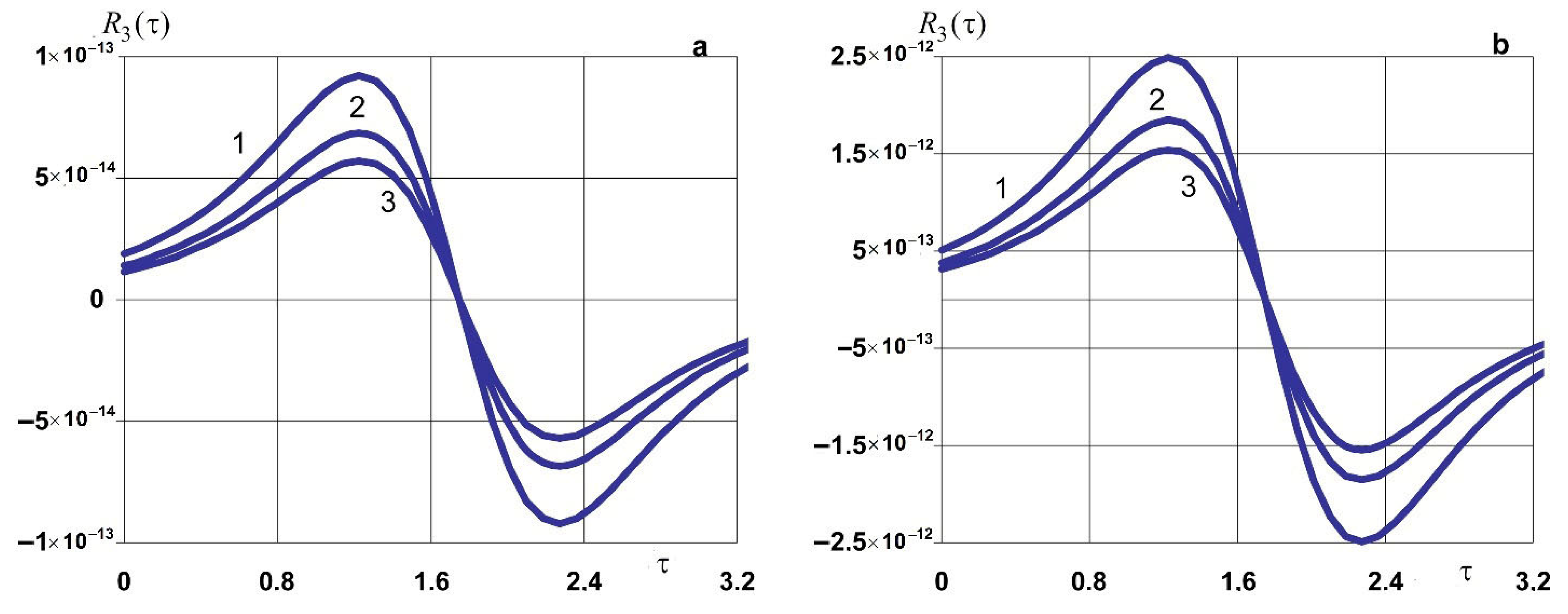
shows the exact values of the function ${\Delta }_f\tilde{f}(\tau )$ and the values of its expansion in the Taylor series (42) with a limit of three terms for three levels of reliability, calculated for $\Delta =$0.001, 0.003 in the interval $\tau \in [0;\hspace{0.17em}3.2]$. Figure 1 demonstrates their corresponding total residual terms $R_3$, calculated by (37), where $\xi$ is the middle of the interval $[t,\tau ]$. Curves 1–3 correspond to the values $\beta =0.9$, 0.95, 0.99 for $\xi (\tau )=$$\tau -0.001$ (Figure 1a) and $\xi (\tau )=$ $\tau -0.003$ (Figure 1b). Since varying the parameters within a wide range gives a similar result $\left|R_3\right|<{10}^{-12}$ (Figure 1); therefore, we assume that the restriction to three terms of the series (41) sufficiently approximates the function ${\Delta }_f\tilde{f}(\tau )$ (37).

In case ${\Delta }_f\tilde{f}(\tau )\approx A_3{\tau }^2+\tilde{b}\tau +\tilde{p}$, where $\tilde{p}=A_1-A_2{a}_1+{A_3{a}_1}^2$, and $\tilde{b}=(A_2-2A_3{a}_1)$, the following is true

$$\begin{gathered} {(-1)}^m{y}_m{e}^{-A{y}_m^2\tau }{\displaystyle \int \tilde{f}(\tau )}\hspace{0.17em}\hspace{0.17em}{e}^{A{y}_m^2\tau }\hspace{0.17em}d\tau ={\displaystyle \frac{{(-1)}^m}{A{y}_m}}\left[A_3{\tau }^2+\tilde{b}\tau +\tilde{p}-{\displaystyle \frac{(2A_3\tau +\tilde{b})}{A{y}_m^2}}+{\displaystyle \frac{2A_3}{A^2{y}_m^4}};\right] \\ {\left.{(-1)}^m{y}_m{\displaystyle \int \tilde{f}(\tau )}\hspace{0.17em}\hspace{0.17em}{e}^{A{y}_m^2\tau }\hspace{0.17em}d\tau \right|}_{\tau =0}={\displaystyle \frac{{(-1)}^m}{A{y}_m}}\left[\tilde{p}-{\displaystyle \frac{\tilde{b}}{A{y}_m^2}}+{\displaystyle \frac{2A_3}{A^2{y}_m^4}}\right]. \end{gathered}$$

Then, for the bilateral critical domain, the following bounds are obtained

$$\begin{gathered} u_f^{\pm }(\tau ,z)=u(\tau ,z)\pm 2B\sqrt{p_1+p_2\tau +q_3{\tau }^2}{\displaystyle \frac{z}{z_0}} \\ \pm {\displaystyle \frac{2}{z_0}}{\displaystyle \sum _{m=1}^{\infty }\frac{{(-1)}^m}{y_m}{e}^{-A{y}_m^2\tau }\left(2B\sqrt{p_1}+A_3{\tau }^2+\tilde{b}\tau -2\frac{(A_3\tau +\tilde{b})}{A{y}_m^2}\right)\sin (y_{m}z)}. \end{gathered}$$

(43)

Consider that $\underset{\tau \to \infty }{\lim }{u}_f^{\pm }(\tau ,z)=\underset{\tau \to \infty }{\lim }u(\tau ,z)\pm 2B\sqrt{p_1+p_2\tau +p_3{\tau }^2}{\displaystyle \frac{z}{z_0}}$. Then, for long-term processes described by the original boundary value problem, the greater the $\tau$, the greater the width of the bilateral critical domain, i.e., functions $u_f^{\pm }(\tau ,z)$ have no stationary mode (time asymptotic). The width of the bilateral critical domain is most influenced by the coefficient $B$. In particular, the smaller the value of $\left|B\right|$, the narrower the two-sided critical domain for the same level of reliability $\beta$. The larger the variance of the predicted value of the linear regression $f(\tau )$, the wider the two-sided critical domain.

8. Influence of Statistical Characteristics of a Sample on Reliable Intervals and Bilateral Critical Domain of a Solution to a Boundary Value Problem

Let us analyze the influence of the statistical characteristics of experimental data on the required function at the lower boundary of the layer using concrete examples. Samples of experimental data were obtained for both the uniform and non-uniform distribution of the study time interval [39]. The basic parameters are $A=1$, $u_{*}=1$, $u_0=0$, and $z_0=1$. The series is calculated with an accuracy of $\epsilon ={10}^{-7}$. Let us consider the cases of samples of large and small volumes characterized by large or small variance.

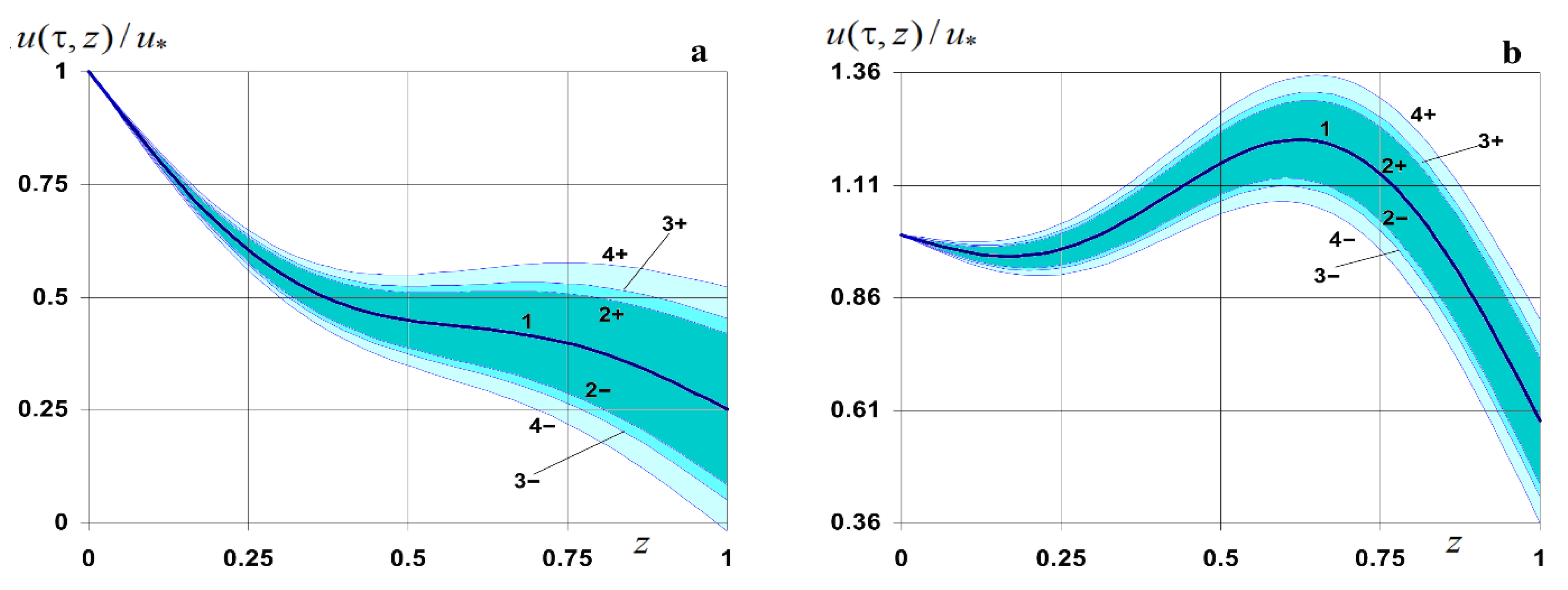
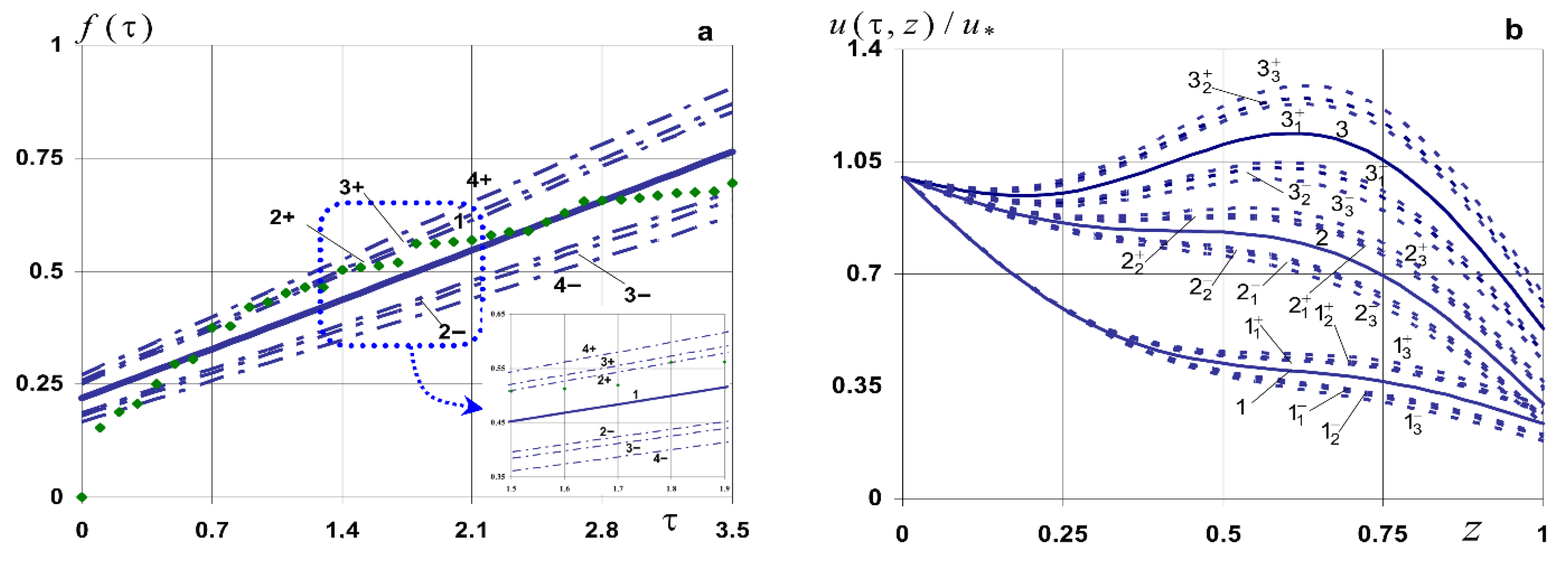
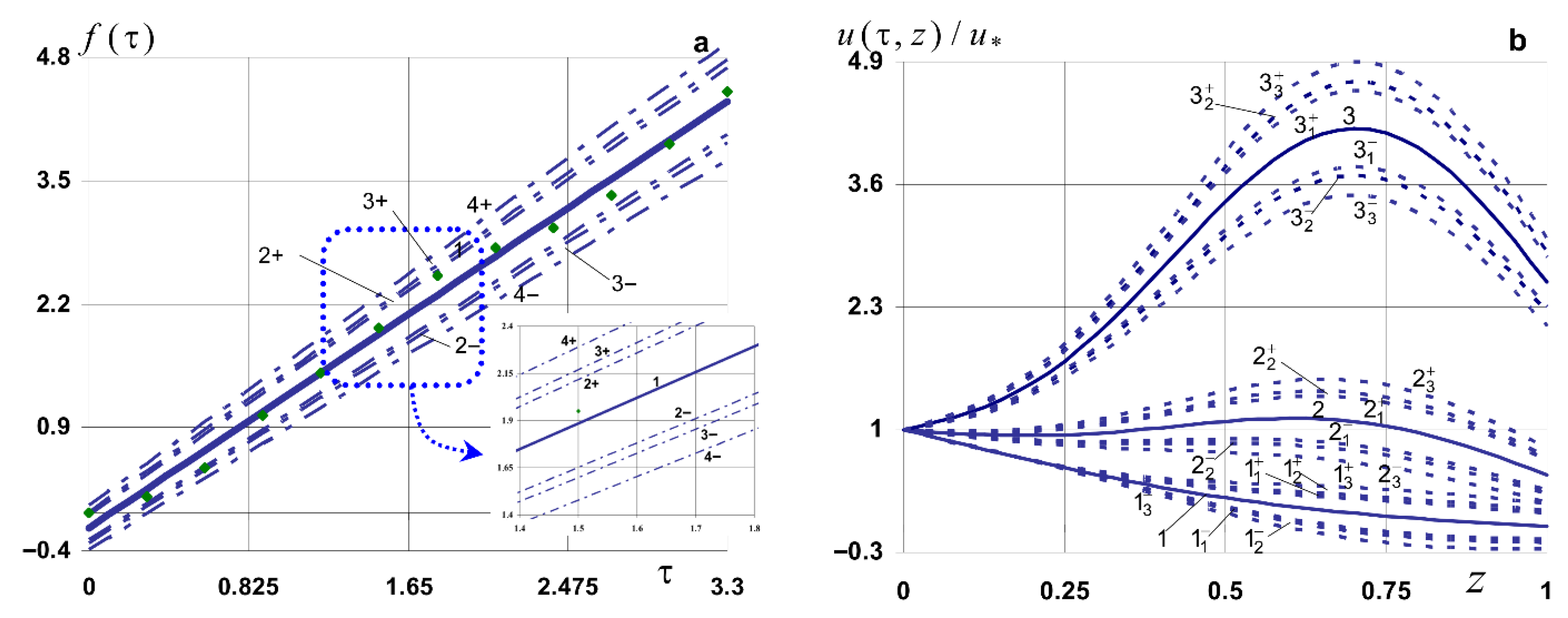
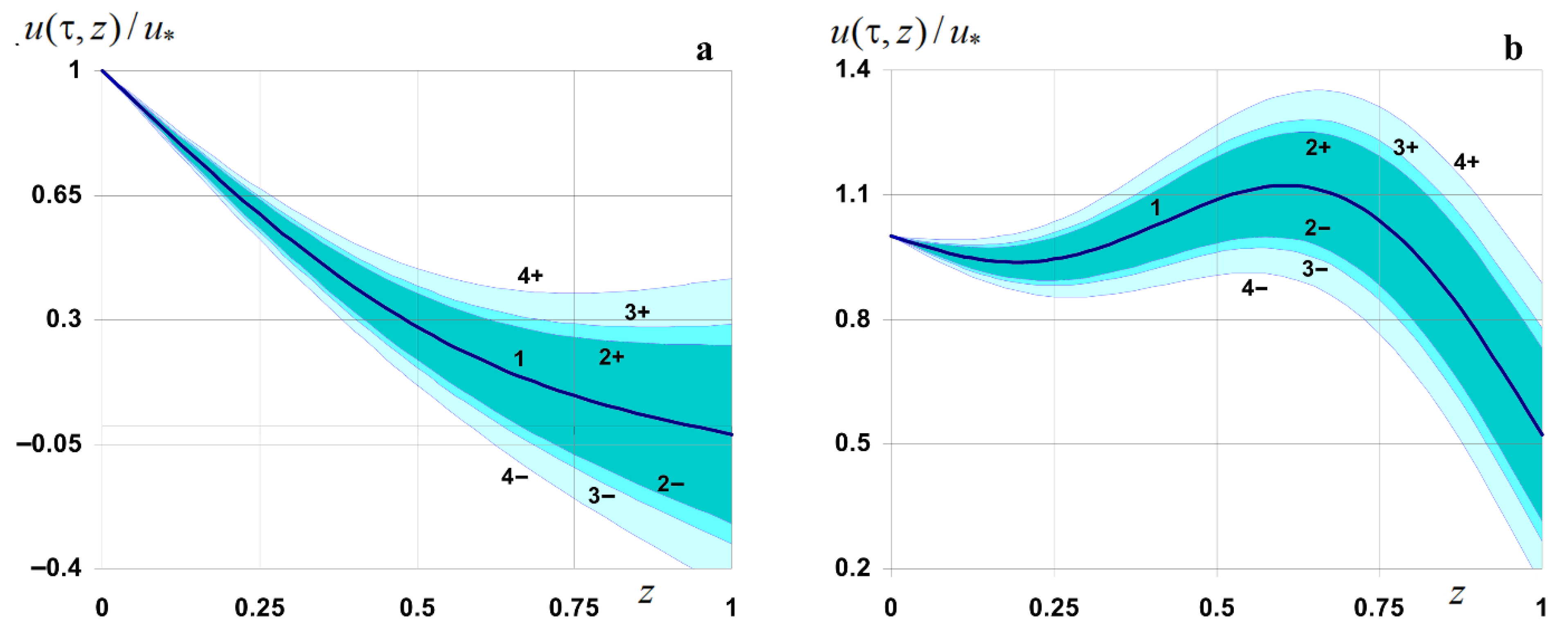
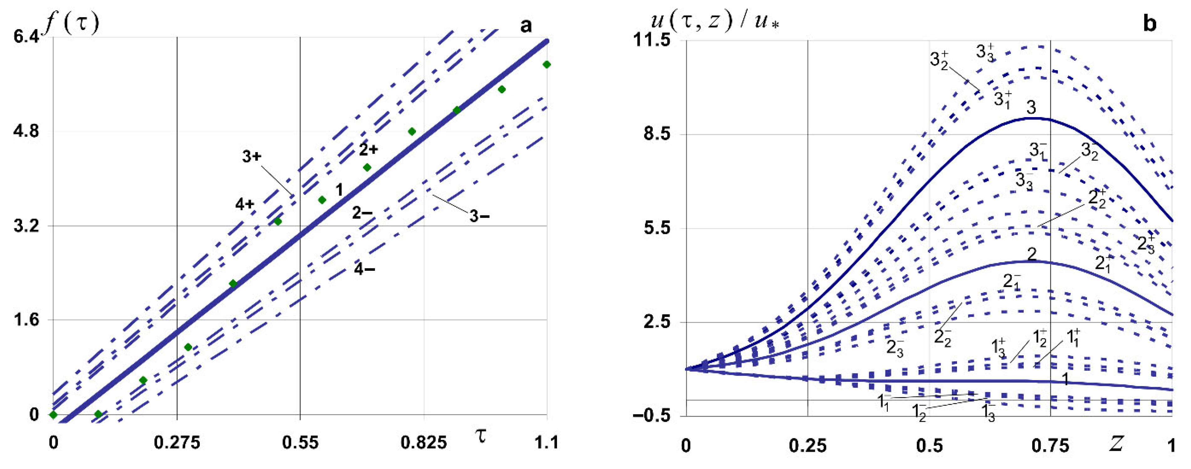
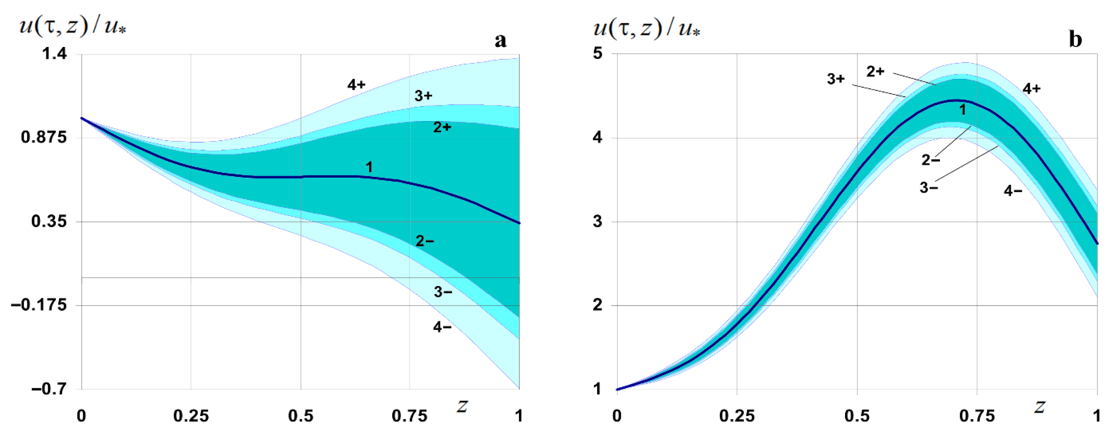
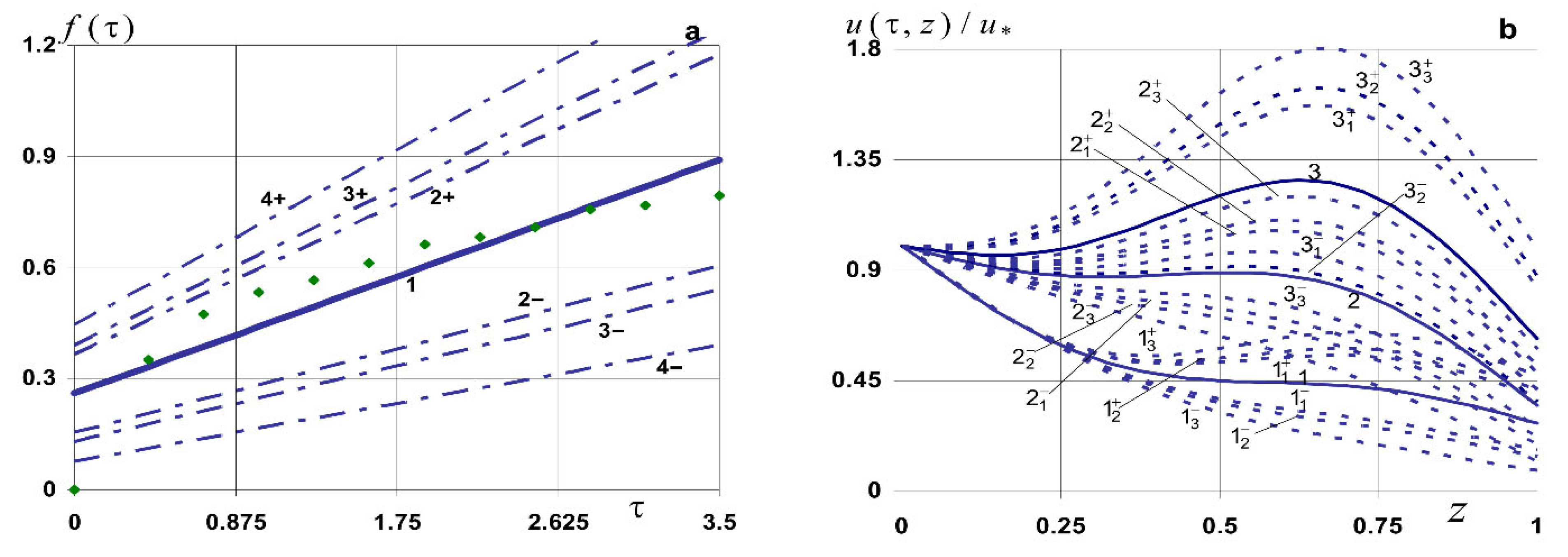
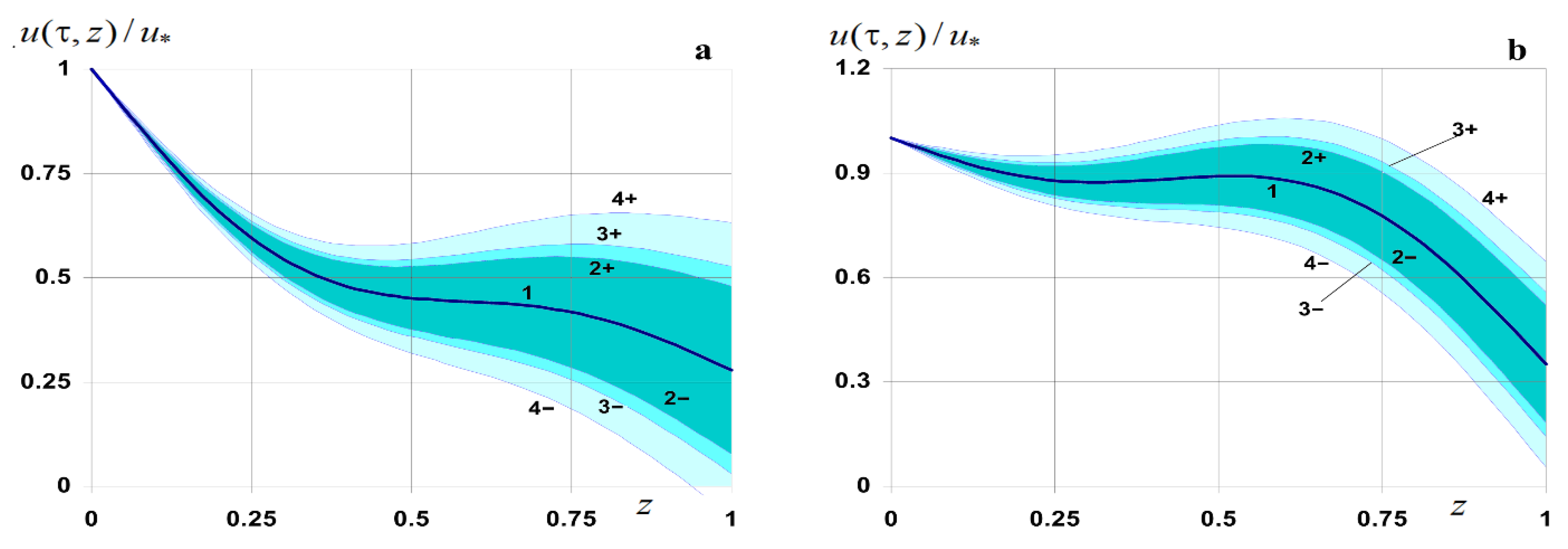
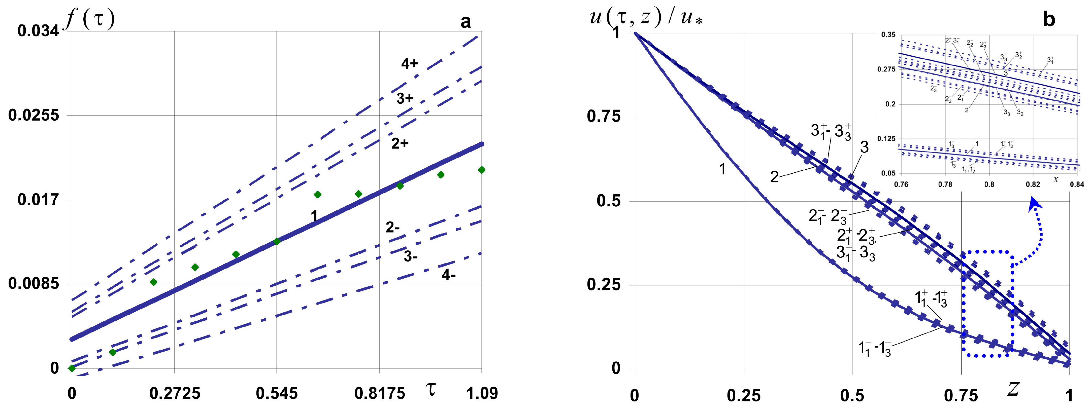
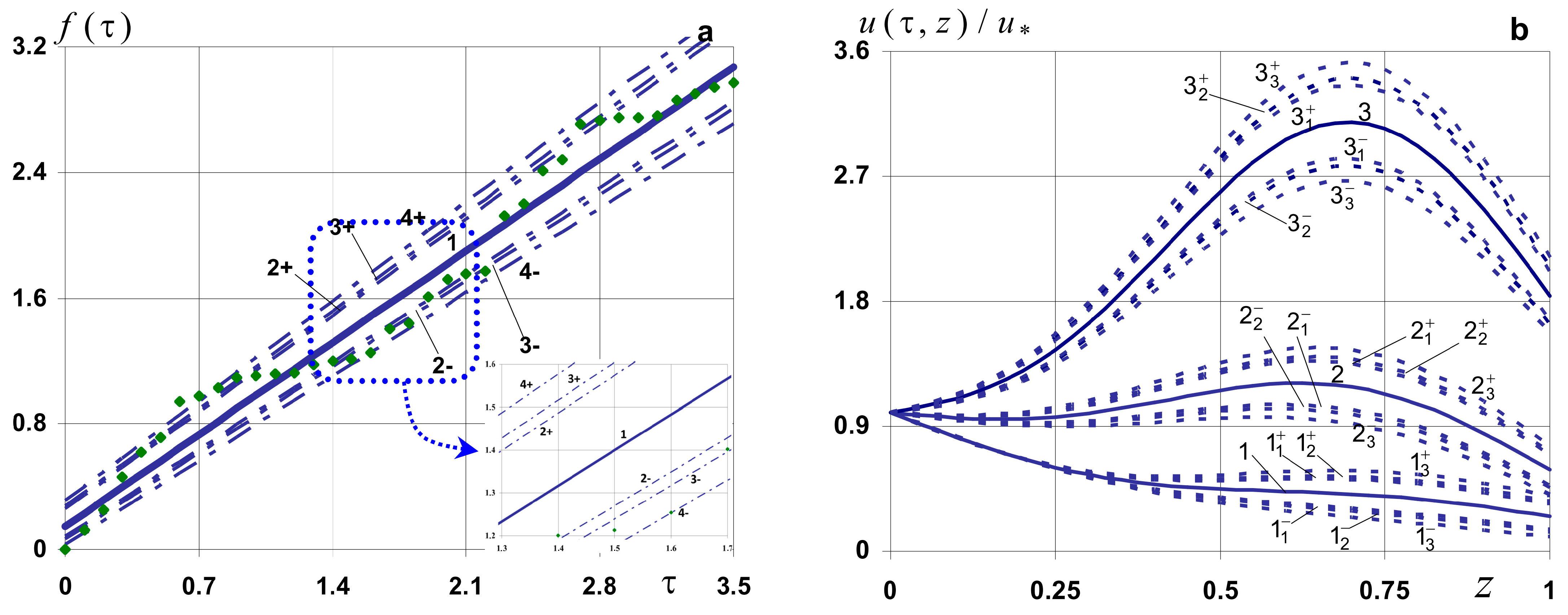
Figures 2, 4, 6, 8, 10, and 12 demonstrate linear regression for the relevant sample (Figures 2a, 4a, 6a, 8a, 10a, and 12a) and solutions to the boundary value problem (1)–(3), (7) (Figures 2b, 4b, 6b, 8b, 10b, and 12b). In Figures 2a, 4a, 6a, 8a, 10a, and 12a, solid lines (curves 1) indicate the function $f(\tau )$, the dashed and dotted lines indicate its reliable intervals $f^{\pm }(\tau )$ (curves 2−, 3−, 4− and 2+, 3+, 4+), and the green dots indicate the experimental data presented in the corresponding table. Figures 2b, 4b, 6b, and 10b show solutions to the initial boundary value problem $u(\tau ,z)$ (solid lines) for long time intervals at time moments $\tau =$0.1, 0.5, 2 (curves 1–3). Figures 8b and 12b show the same solutions for short time intervals at time moments $\tau =$0.1, 0.5, 1 (curves 1–3). The curves (dashed lines) with the index “+” are calculated for the upper limits of the reliable intervals $u_c^{+}(\tau ,z)$, and with the index “−” for the lower ones $u_c^{-}(\tau ,z)$. The lower indices 1, 2, 3 correspond to the values of the reliability level $\beta =0.9$, 0.95, 0.99. Figures 3, 5, 7, 9, 11 and 13 show solutions to the initial boundary value problem $u(\tau ,z)$, that are normalized to the value of the function on the upper boundary of the layer $z=0$, and the corresponding bilateral critical domains calculated by the Fisher criterion, for $\tau =$0.1 (Figures 3a, 5a, 7a, 9a, 11a and 13a) and $\tau =$0.5 (Figures 3b, 5b, 7b, 9b, 11b and 13b). Curves 2−, 2+ are calculated for $\beta =0.9$, curves 3−, 3+ are calculated for $\beta =0.95$, and curves 4−, 4+ are calculated for $\beta =0.99$.

Tables 4, 6, 8, 10, 12 and 14 contain the maximum widths of the two-sided critical domain of the boundary value problem (1)–(3), (7) ${\Delta }_c(\tau ,z)={\displaystyle \frac{1}{u_{*}}}\left|u_c^{+}(\tau ,z)-u_c^{-}(\tau ,z)\right|$ for different time moments $\tau$ and $\beta =0.9$, 0.95, 0.99 for six samples.

8.1. Sample I: Large Sample, Long Time Interval, Large Variance

Sample of experimental data $f(\tau )$ with volume $n=36$ is shown in

Table 3. Experimental data with a large variance over a long time interval for $n=36$.

	${\tau }_1$	${\tau }_2$	${\tau }_3$	${\tau }_4$	${\tau }_5$	${\tau }_6$	${\tau }_7$	${\tau }_8$	${\tau }_9$	${\tau }_{10}$	${\tau }_{11}$	${\tau }_{12}$
${\tau }_i$	0	0.1	0.2	0.3	0.4	0.5	0.6	0.7	0.8	0.9	1	1.1
$f({\tau }_i)$	0	0.121	0.2527	0.4609	0.6212	0.7142	0.9401	0.9771	1.0312	1.0922	1.1052	1.1197
	${\tau }_{13}$	${\tau }_{14}$	${\tau }_{15}$	${\tau }_{16}$	${\tau }_{17}$	${\tau }_{18}$	${\tau }_{19}$	${\tau }_{20}$	${\tau }_{21}$	${\tau }_{22}$	${\tau }_{23}$	${\tau }_{24}$
${\tau }_i$	1.2	1.3	1.4	1.5	1.6	1.7	1.8	1.9	2	2.1	2.2	2.3
$f({\tau }_i)$	1.1254	1.1741	1.2005	1.2129	1.2539	1.4017	1.4387	1.6109	1.7208	1.7562	1.7707	2.1208
	${\tau }_{25}$	${\tau }_{26}$	${\tau }_{27}$	${\tau }_{28}$	${\tau }_{29}$	${\tau }_{30}$	${\tau }_{31}$	${\tau }_{32}$	${\tau }_{33}$	${\tau }_{34}$	${\tau }_{35}$	${\tau }_{36}$
${\tau }_i$	2.4	2.5	2.6	2.7	2.8	2.9	3	3.1	3.2	3.3	3.4	3.5
$f({\tau }_i)$	2.2022	2.4131	2.4799	2.7115	2.7307	2.7471	2.7517	2.7641	2.8615	2.9029	2.9413	2.9716

.

The sample range is $R$ = [0, 2.9716], and the sample variance is $S_f^2$ = 0.893931523259907. Let us build a regression based on the data in Table 3 using the least squares method. Based on the view of the correlation field, we assume that the time dependence of the required function on the lower boundary of the body ${\left.u(\tau )\right|}_{z_0}$ is linear. According to the sample data, the coefficients of the linear regression (4) are $a_1$ = 0.835387001287001 and $a_0$ = 0.16861996996997. Now, let us find reliable intervals with reliability $\beta$ for the linear regression coefficients. For the coefficients $a_1$ and $a_0$ reliable intervals with reliability $\beta =0.9$ are calculated within reliable limits $a_1\in$ (0.792324843411; 0.878449159163); $a_0\in$ (0.080983805814; 0.256256134126); with reliability $\beta =0.95$ are calculated within reliable limits $a_1\in$ (0.783632562191029; 0.887141440382974); $a_0\in$ (0.063294070291443; 0.273945869648497); with reliability $\beta =0.99$ are calculated within reliable limits $a_1\in$ (0.765903964133865; 0.904870038440137); and $a_0\in$ (0.0272144494313441; 0.310025490508596). For short times of the transfer process described by the boundary value problem (1)–(3), (7), the function $u(\tau ,z)$ monotonically decreases (curve 1, Figure 2b). As increasing $\tau$ values of the function also increase, the maximum is formed at the point $z_{\max }=0.625$ (curve 2, Figure 2b). This maximum eventually shifts to the lower boundary of the body, for example ${\left.z_{\max }\right|}_{\tau =2}=0.7$. Afterwards, the behavior of the function $u(\tau ,z)$ but its values in the entire body area increase significantly (curve 3, Figure 2b). Boundaries of the bilateral critical domain $u_f^{\pm }(\tau ,z)$, calculated by Formula (43), for this sample and all others are given in Appendix A.

As the transfer time increases, not only do the values $u(\tau ,z)$ increase, but the widths of the reliable intervals also increase ${\Delta }_c(\tau ,z)$ (Figure 2b). Thus, with an increase in $\tau$ value from 0.5 to 2, the maximum widths of the reliable intervals increase more than double, regardless of the value of $\beta$. For example, ${\left.\underset{z\in [0,z_0]}{\max }{\Delta }_c(\tau ,z)\right|}_{\begin{array}{l}\tau =2\\ \beta =0.99\end{array}}/{\left.\underset{z\in [0,z_0]}{\max }{\Delta }_c(\tau ,z)\right|}_{\begin{array}{l}\tau =0.5\\ \beta =0.99\end{array}}=1.59$. At the same time, increasing the level of reliability $\beta$ from 0.9 to 0.99 leads to the expansion of the reliable interval to 61%. In particular, ${\left.\underset{z\in [0,z_0]}{\max }{\Delta }_c(\tau ,z)\right|}_{\begin{array}{l}\tau =3\\ \beta =0.99\end{array}}/{\left.\underset{z\in [0,z_0]}{\max }{\Delta }_c(\tau ,z)\right|}_{\begin{array}{l}\tau =3\\ \beta =0.9\end{array}}=1.61$.

In contrast to the reliable intervals, the bilateral critical domain of the problem solution initially decreases (Figure 3), reaching its narrowest values in the middle of the time interval $[0,{\tau }_n]$; further, the bilateral critical domain expands, symmetrically to the narrowing in the initial time interval (

Table 4. Maximum width of the two-sided critical solution domain for sample I.

$\mathit{\tau }$	0.1	0.8	1.4	1.7	2.2	2.7	3.4
$\underset{z\in [0,z_0]}{\max }{\Delta }_f(\tau ,z)$ $\beta =0.9$	0.335848	0.242477	0.188819	0.179144	0.195004	0.242477	0.335848
$\underset{z\in [0,z_0]}{\max }{\Delta }_f(\tau ,z)$ $\beta =0.95$	0.40364	0.291422	0.226934	0.215305	0.234366	0.291422	0.40364
$\underset{z\in [0,z_0]}{\max }{\Delta }_f(\tau ,z)$ $\beta =0.99$	0.541908	0.39125	0.304670	0.289058	0.314648	0.39125	0.541908

). Thus, for short times, the width of this domain ${\Delta }_f(\tau ,z)={\displaystyle \frac{1}{u_{*}}}\left|u_f^{+}(\tau ,z)-u_f^{-}(\tau ,z)\right|$ decreases to 17%, namely ${\left.\underset{z\in [0,z_0]}{\max }{\Delta }_f(\tau ,z)\right|}_{\tau =0.5}/{\left.\underset{z\in [0,z_0]}{\max }{\Delta }_f(\tau ,z)\right|}_{\tau =0.1}=$0.833 for $\forall \beta$ (Figure 3a,b); for medium times, the difference between ${\left.\underset{z\in [0,z_0]}{\max }{\Delta }_f(\tau ,z)\right|}_{\tau =1}$ and ${\left.\underset{z\in [0,z_0]}{\max }{\Delta }_f(\tau ,z)\right|}_{\tau =2}$ decreases by 16.6%. The largest widths of the bilateral critical domain at increasing $\beta$ increase by 60%. For example, ${\left.\underset{z\in [0,z_0]}{\max }{\Delta }_f(\tau ,z)\right|}_{\begin{array}{l}\tau =3\\ \beta =0.99\end{array}}/{\left.\underset{z\in [0,z_0]}{\max }{\Delta }_f(\tau ,z)\right|}_{\begin{array}{l}\tau =3\\ \beta =0.9\end{array}}=1.6$.

8.2. Sample II: Large Sample, Long Time Interval, Small Variance

Sample of experimental data $f(\tau )$ with volume $n=36$ is shown in

Table 5. Experimental data with low variance for a long time interval.

	${\tau }_1$	${\tau }_2$	${\tau }_3$	${\tau }_4$	${\tau }_5$	${\tau }_6$	${\tau }_7$	${\tau }_8$	${\tau }_9$	${\tau }_{10}$	${\tau }_{11}$	${\tau }_{12}$
${\tau }_i$	0	0.1	0.2	0.3	0.4	0.5	0.6	0.7	0.8	0.9	1	1.1
$f({\tau }_i)$	0	0.153	0.188	0.207	0.251	0.295	0.306	0.374	0.378	0.42	0.432	0.451
	${\tau }_{13}$	${\tau }_{14}$	${\tau }_{15}$	${\tau }_{16}$	${\tau }_{17}$	${\tau }_{18}$	${\tau }_{19}$	${\tau }_{20}$	${\tau }_{21}$	${\tau }_{22}$	${\tau }_{23}$	${\tau }_{24}$
${\tau }_i$	1.2	1.3	1.4	1.5	1.6	1.7	1.8	1.9	2	2.1	2.2	2.3
$f({\tau }_i)$	0.464	0.465	0.502	0.508	0.512	0.519	0.561	0.562	0.565	0.568	0.58	0.586
	${\tau }_{25}$	${\tau }_{26}$	${\tau }_{27}$	${\tau }_{28}$	${\tau }_{29}$	${\tau }_{30}$	${\tau }_{31}$	${\tau }_{32}$	${\tau }_{33}$	${\tau }_{34}$	${\tau }_{35}$	${\tau }_{36}$
${\tau }_i$	2.4	2.5	2.6	2.7	2.8	2.9	3	3.1	3.2	3.3	3.4	3.5
$f({\tau }_i)$	0.589	0.609	0.628	0.654	0.656	0.659	0.662	0.668	0.672	0.674	0.677	0.694

.

The sample range is $R=$ [0. 0.694], and sample variance is $S_f^2$ = 0.174264028380218.

For the regression coefficients $a_1$ = 0.155924066924067 and $a_0$ = 0.218493993993994, reliable intervals with reliability $\beta =0.9$ are calculated within the following reliable limits $a_1\in$ (0.139918763614950; 0.171929370233184); $a_0\in$ (0.185921464949008; and 0.251066523038980); with reliability $\beta =0.95$ are calculated within the following reliable limits $a_1\in$ (0.136688; 0.17516); and $a_0\in$ (0.179346560289016; 0.257641427698971); with reliability $\beta =0.99$ are calculated within the following reliable limits $a_1\in$ (0.130098675459337; 0.181749458388797); and $a_0\in$ (0.165936519928265; 0.271051468059722).

As the transfer process increases in time, the function value $u(\tau ,z)$ increases in the entire body area (Figure 4b). For short and mid-long times $u(\tau ,z)$ is a monotonically decreasing function. The local maximum of the function begins to form at moment $\tau =$0.6 in the point $z_{\max }=0.55$. With the increase in $t$ this maximum grows, shifting to the lower boundary of the layer (${\left.z_{\max }\right|}_{\tau =2}=0.6$) and becomes global (Figure 4b). With the increase in time, the width of the reliable interval ${\Delta }_c(\tau ,z)$ grows (Figure 4b), similarly for different values $\beta$. For example, ${\left.\underset{z\in [0,z_0]}{\max }{\Delta }_c(\tau ,z)\right|}_{\begin{array}{l}\tau =2\\ \beta =0.9\end{array}}/{\left.\underset{z\in [0,z_0]}{\max }{\Delta }_c(\tau ,z)\right|}_{\begin{array}{l}\tau =0.5\\ \beta =0.9\end{array}}=$${\left.=\underset{z\in [0,z_0]}{\max }{\Delta }_c(\tau ,z)\right|}_{\begin{array}{l}\tau =2\\ \beta =0.99\end{array}}/{\left.\underset{z\in [0,z_0]}{\max }{\Delta }_c(\tau ,z)\right|}_{\begin{array}{l}\tau =0.5\\ \beta =0.99\end{array}}=1.598$.

The two-sided critical domain of the sample is also initially narrowed (Figure 5), and then, in the second half of the time interval $[0,{\tau }_n]$ is extended (

Table 6. Maximum width of the two-sided critical solution domain for sample II.

$\mathit{\tau }$	0.1	0.8	1.4	1.7	2.2	2.7	3.4
$\underset{z\in [0,z_0]}{\max }{\Delta }_f(\tau ,z)$ $\beta =0.9$	0.12482769	0.0901237	0.0701804	0.066584	0.0724789	0.0901237	0.12482769
$\underset{z\in [0,z_0]}{\max }{\Delta }_f(\tau ,z)$ $\beta =0.95$	0.15002469	0.1083156	0.08434663	0.0800244	0.08710905	0.108315603	0.15002469
$\underset{z\in [0,z_0]}{\max }{\Delta }_f(\tau ,z)$ $\beta =0.99$	0.20141598	0.1454194	0.1132398	0.10743694	0.1169484	0.1454194	0.20141598

). The width of this domain ${\Delta }_f(\tau ,z)$ for short times decreases to 17%, namely ${\left.\underset{z\in [0,z_0]}{\max }{\Delta }_f(\tau ,z)\right|}_{\tau =0.5}/{\left.\underset{z\in [0,z_0]}{\max }{\Delta }_f(\tau ,z)\right|}_{\tau =0.1}=$0.833 for $\forall \beta$ (Figure 5); for long times, the difference between ${\left.\underset{z\in [0,z_0]}{\max }{\Delta }_f(\tau ,z)\right|}_{\tau =1}$ and ${\left.\underset{z\in [0,z_0]}{\max }{\Delta }_f(\tau ,z)\right|}_{\tau =2}$ decreases by 16.6%. There is also symmetry in the widths ${\Delta }_f(\tau ,z)$ in time intervals $[0,{\tau }_n/2]$ and $[{\tau }_n/2,{\tau }_n]$. The largest widths of the bilateral critical domain at increasing $\beta$ increase by 60% too. For example, ${\left.\underset{z\in [0,z_0]}{\max }{\Delta }_f(\tau ,z)\right|}_{\begin{array}{l}\tau =3\\ \beta =0.99\end{array}}/{\left.\underset{z\in [0,z_0]}{\max }{\Delta }_f(\tau ,z)\right|}_{\begin{array}{l}\tau =3\\ \beta =0.9\end{array}}=1.6$. For samples I and II, the growth rate of the reliable interval ${\Delta }_c(\tau ,z)$ and reduction in the bilateral critical domain ${\Delta }_f(\tau ,z)$, and then the corresponding growth is the same.

8.3. Sample III: Small Sample, Long Time Interval, Large Variance

Sample of experimental data $f(\tau )$ with volume $n=12$ is shown in

Table 7. Experimental data with a large variance over a long time interval for $n=12$.

	${\tau }_1$	${\tau }_2$	${\tau }_3$	${\tau }_4$	${\tau }_5$	${\tau }_6$	${\tau }_7$	${\tau }_8$	${\tau }_9$	${\tau }_{10}$	${\tau }_{11}$	${\tau }_{12}$
${\tau }_i$	0	0.3	0.6	0.9	1.2	1.5	1.8	2.1	2.4	2.7	3	3.3
$f({\tau }_i)$	0	0.1697	0.4738	1.0209	1.4735	1.9513	2.4972	2.7988	2.9986	3.3457	3.8914	4.4371

.

The sample range is $R=$ [0, 4.4371], and sample variance is $S_f^2$ = 1.47815809975753. For regression coefficients $a_1=$ 1.361503496503 and $a_0$ = −0.158314102564102 reliable intervals with reliability $\beta =0.9$ are calculated within the following reliable limits $a_1\in$ (1.2942027604045400; 1.4288042326024500); and $a_0\in$ (−0.289421049582769; −0.0272071555454357); with reliability $\beta =0.95$ are calculated within the following reliable limits $a_1\in$ (1.27876771583259; 1.4442392771744); and $a_0\in$ (−0.319489689069116; 0.00286148394091157); with reliability $\beta =0.99$ are calculated within the following reliable limits $a_1\in$ (1.24382131097189; 1.47918568203511); and $a_0\in$ (−0.387567940751664; 0.0709397356234593). For the experimental data on the values of the required function at the lower boundary of the layer, presented in Table 7, also for short transfer times, the function $u(\tau ,z)$ monotonically decreases (Curve 1, Figure 6b). As increasing $\tau$ values of the function increase and the maximum is formed at the point $z_{\max }=0.55$ (Curve 2, Figure 6b), that grows over time and shifts to the lower boundary of the layer. In particular, at $t=2$ the maximum value of the function is reached at the point $z_{\max }=0.7$. For long times, the values of the function $u(\tau ,z)$ increase significantly in the entire body domain (Curve 3, Figure 6b). With the prolongation of time, the width of the reliable interval ${\Delta }_c(\tau ,z)$ increases (Figure 6b), in the same way for different values $\beta$.

For example,

$${\left.\underset{z\in [0,z_0]}{\max }{\Delta }_c(\tau ,z)\right|}_{\begin{array}{l}\tau =2\\ \beta =0.9\end{array}}/{\left.\underset{z\in [0,z_0]}{\max }{\Delta }_c(\tau ,z)\right|}_{\begin{array}{l}\tau =0.5\\ \beta =0.9\end{array}}={\left.\underset{z\in [0,z_0]}{\max }{\Delta }_c(\tau ,z)\right|}_{\begin{array}{l}\tau =2\\ \beta =0.99\end{array}}/{\left.\underset{z\in [0,z_0]}{\max }{\Delta }_c(\tau ,z)\right|}_{\begin{array}{l}\tau =0.5\\ \beta =0.99\end{array}}=1.52.$$

The bilateral critical domain of the problem solution also reduces over time (Figure 7) and then expands (

Table 8. Maximum width of the two-sided critical solution domain for sample III.

$\mathit{\tau }$	0.1	0.8	1.4	1.7	2.2	2.5	3.2
$\underset{z\in [0,z_0]}{\max }{\Delta }_f(\tau ,z)$ $\beta =0.9$	0.50183068	0.3606716	0.28679907	0.2791155	0.31566844	0.3606716	0.50183068
$\underset{z\in [0,z_0]}{\max }{\Delta }_f(\tau ,z)$ $\beta =0.95$	0.61692272	0.4433896	0.3525748	0.34312913	0.3880652	0.4433896	0.61692272
$\underset{z\in [0,z_0]}{\max }{\Delta }_f(\tau ,z)$ $\beta =0.99$	0.87750201	0.6306711	0.50149735	0.488061947	0.55197837	0.6306711	0.87750201

) for this sample. The width of this domain ${\Delta }_f(\tau ,z)$ for short times decreases to 17%, namely ${\left.\underset{z\in [0,z_0]}{\max }{\Delta }_f(\tau ,z)\right|}_{\tau =0.5}/{\left.\underset{z\in [0,z_0]}{\max }{\Delta }_f(\tau ,z)\right|}_{\tau =0.1}=0.830$ for $\forall \beta$ (Figure 7); for long times, the difference between ${\left.\underset{z\in [0,z_0]}{\max }{\Delta }_f(\tau ,z)\right|}_{\tau =1}$ and ${\left.\underset{z\in [0,z_0]}{\max }{\Delta }_f(\tau ,z)\right|}_{\tau =2}$ decreases by 10.6%. The larger widths of the bilateral critical domain with increasing $\beta$ increase by 75%. For example, ${\left.\underset{z\in [0,z_0]}{\max }{\Delta }_f(\tau ,z)\right|}_{\begin{array}{l}\tau =3\\ \beta =0.99\end{array}}/{\left.\underset{z\in [0,z_0]}{\max }{\Delta }_f(\tau ,z)\right|}_{\begin{array}{l}\tau =3\\ \beta =0.9\end{array}}=1.75$. Symmetry in relation to the widths ${\Delta }_f(\tau ,z)$ of time intervals $[0,{\tau }_n/2]$ and $[{\tau }_n/2,{\tau }_n]$ is also present.

8.4. Sample IV: Small Sample, Short Time Interval, Large Variance

Let us now consider a sample of experimental data $f(\tau )$ with volume $n=12$ over a short time interval, as

Table 9. Experimental data with a large variance over a short time interval.

	${\tau }_1$	${\tau }_2$	${\tau }_3$	${\tau }_4$	${\tau }_5$	${\tau }_6$	${\tau }_7$	${\tau }_8$	${\tau }_9$	${\tau }_{10}$	${\tau }_{11}$	${\tau }_{12}$
${\tau }_i$	0	0.1	0.2	0.3	0.4	0.5	0.6	0.7	0.8	0.9	1.0	1.1
$f({\tau }_i)$	0	0.0162	0.5809	1.1439	2.2175	3.2737	3.6345	4.1847	4.8021	5.1542	5.5129	5.9291

shows.

Sample range $R=$ [0, 5.9291], and sample variance $S_f^2$ = 2.18380650788105. For the regression coefficients $a_1=$ 5.9880034965035 and $a_0$ = −0.2559269230769220 reliable intervals with reliability $\beta =0.9$ are calculated within the following reliable limits $a_1\in$ (5.4663064488105100; 6.5097005441964900); and $a_0\in$ (−0.5946954178281560; 0.0828415716743118); with reliability $\beta =0.95$ are calculated within the following reliable limits $a_1\in$ (5.34665817078342; 6.62934882222358); and $a_0\in$ (−0.672390063074964; 0.16053621692112); with reliability $\beta =0.99$ are calculated within the following reliable limits $a_1\in$ (5.07576312118831; 6.90024387181869); and $a_0\in$ (−0.848298108927857; 0.336444262774013).

For the experimental data on the values of the required function at the lower boundary of the layer, presented in Table 9, the formation of a local maximum of the function $u(\tau ,z)$ already begins for short times. This $\underset{z\in [0,z_0]}{\max }u(\tau ,z)$ forms in the middle of the body, grows over time, and shifts to the lower border of the layer. For example, ${\left.z_{\max }\right|}_{\tau =0.1}=0.575$ and $\underset{z\in [0,z_0]}{\max }u(\tau ,z)=$ 0.635718339 (Curve 1, Figure 8b), ${\left.z_{\max }\right|}_{\tau =0.5}=0.7$ and $\underset{z\in [0,z_0]}{\max }u(\tau ,z)=$ 4.4428612 (Curve 2, Figure 8b), ${\left.z_{\max }\right|}_{\tau =1}=0.725$ and $\underset{z\in [0,z_0]}{\max }u(\tau ,z)=$ 9.007544363 (Curve 3, Figure 8b). The reliable interval width ${\Delta }_c(\tau ,z)$ with the prolongation of the process time increases (Figure 8b), and is the same for the different values $\beta$. For example, ${\left.\underset{z\in [0,z_0]}{\max }{\Delta }_c(\tau ,z)\right|}_{\begin{array}{l}\tau =1\\ \beta =0.9\end{array}}/{\left.\underset{z\in [0,z_0]}{\max }{\Delta }_c(\tau ,z)\right|}_{\begin{array}{l}\tau =0.5\\ \beta =0.9\end{array}}=$${\left.\underset{z\in [0,z_0]}{\max }{\Delta }_c(\tau ,z)\right|}_{\begin{array}{l}\tau =1\\ \beta =0.99\end{array}}/{\left.\underset{z\in [0,z_0]}{\max }{\Delta }_c(\tau ,z)\right|}_{\begin{array}{l}\tau =0.5\\ \beta =0.99\end{array}}=$ 1.93. For this sample, the bilateral critical domain of the solution also narrows with time (Figure 9), and then enlarges symmetrically on the intervals $[0,{\tau }_n/2]$ and $[{\tau }_n/2,{\tau }_n]$ (

Table 10. Maximum width of the two-sided critical solution domain for sample IV.

$\mathit{\tau }$	0.1	0.3	0.5	0.6	0.7	0.8	1
$\underset{z\in [0,z_0]}{\max }{\Delta }_f(\tau ,z)$ $\beta =0.9$	1.183536	0.8894386	0.7278873	0.7278873	0.7854385	0.8894386	1.183536
$\underset{z\in [0,z_0]}{\max }{\Delta }_f(\tau ,z)$ $\beta =0.95$	1.4549728	1.0934262	0.8948241	0.8948241	0.9655743	1.0934262	1.4549728
$\underset{z\in [0,z_0]}{\max }{\Delta }_f(\tau ,z)$ $\beta =0.99$	2.0695327	1.55527397	1.2727851	1.2727851	1.37341921	1.55527397	2.0695327

). The width of this domain ${\Delta }_f(\tau ,z)$ for short times reduces to 25%, namely ${\left.\underset{z\in [0,z_0]}{\max }{\Delta }_f(\tau ,z)\right|}_{\tau =0.3}/{\left.\underset{z\in [0,z_0]}{\max }{\Delta }_f(\tau ,z)\right|}_{\tau =0.1}$ = 0.75 for $\forall \beta$ (Figure 9); for medium times, the difference between ${\left.\underset{z\in [0,z_0]}{\max }{\Delta }_f(\tau ,z)\right|}_{\tau }$ = 0.5 and ${\left.\underset{z\in [0,z_0]}{\max }{\Delta }_f(\tau ,z)\right|}_{\tau =1}$ increases by 61.5%. The largest widths of the bilateral critical domain at increasing $\beta$ also increase by 75%. For example, ${\left.\underset{z\in [0,z_0]}{\max }{\Delta }_f(\tau ,z)\right|}_{\begin{array}{l}\tau =1\\ \beta =0.99\end{array}}/{\left.\underset{z\in [0,z_0]}{\max }{\Delta }_f(\tau ,z)\right|}_{\begin{array}{l}\tau =1\\ \beta =0.9\end{array}}=1.75.$

8.5. Sample V: Small Sample, Long Time Interval, Small Variance

Sample of experimental data $f(\tau )$ with volume $n=12$ is obtained over a long time interval.

Sample range $R=$ [0, 0.794], and sample variance $S_f^2$ = 0.223456914022016. For the regression coefficients $a_1$ = 0.180180811808118 and $a_0$ = 0.26010024600246 reliable intervals with reliability $\beta =0.9$ are calculated within the following reliable limits $a_1\in$ (0.128690059337185; 0.231671564279051); and $a_0\in$ (0.154680344031757; 0.365520147973162); with reliability $\beta =0.95$ are calculated within the following reliable limits $a\in$ (0.116880945418082; 0.243480678198154); and $a_0\in$ (0.130502883575815; 0.389697608429105); with reliability $\beta =0.99$ are calculated within the following reliable limits $a_1\in$ (0.0901439914598696; 0.270217632156367); and $a_0\in$ (0.0757628199719453; 0.444437672032974). For the experimental data on the values of the required function at the lower boundary of the layer, presented in

Table 11. Experimental data with low variance over a long time interval.

	${\tau }_1$	${\tau }_2$	${\tau }_3$	${\tau }_4$	${\tau }_5$	${\tau }_6$	${\tau }_7$	${\tau }_8$	${\tau }_9$	${\tau }_{10}$	${\tau }_{11}$	${\tau }_{12}$
${\tau }_i$	0	0.4	0.7	1	1.3	1.6	1.9	2.2	2.5	2.8	3.1	3.5
$f({\tau }_i)$	0	0.351	0.474	0.532	0.565	0.612	0.662	0.682	0.709	0.756	0.768	0.794

, for short times, the function $u(\tau ,z)$ monotonically decreases (Curve 1, Figure 10b). The local maximum of the function $u(\tau ,z)$ is formed at the point $z_{\max }=0.525$ (Curve 2, Figure 10b) and, as in the previous cases, increases with time and shifts to the lower boundary of the layer (Curve 3, Figure 10b). For example, ${\left.z_{\max }\right|}_{\tau =2}=0.625$ and $\underset{z\in [0,z_0]}{\max }u(\tau ,z)=1.267372491$ (Curve 3, Figure 10b).

Reliable interval width ${\Delta }_c(\tau ,z)$ with the prolongation of the process time increases (Figure 10b); moreover, this occurs in the same manner for the different values $\beta$. For example, ${\left.\underset{z\in [0,z_0]}{\max }{\Delta }_c(\tau ,z)\right|}_{\begin{array}{l}\tau =2\\ \beta =0.9\end{array}}/{\left.\underset{z\in [0,z_0]}{\max }{\Delta }_c(\tau ,z)\right|}_{\begin{array}{l}\tau =0.5\\ \beta =0.9\end{array}}=$${\left.\underset{z\in [0,z_0]}{\max }{\Delta }_c(\tau ,z)\right|}_{\begin{array}{l}\tau =2\\ \beta =0.99\end{array}}/{\left.\underset{z\in [0,z_0]}{\max }{\Delta }_c(\tau ,z)\right|}_{\begin{array}{l}\tau =0.5\\ \beta =0.99\end{array}}=1.59.$

For this sample, the bilateral critical domain of the solution of the problem also narrows with time (Figure 11), and then widens symmetrically in the intervals $[0,{\tau }_n/2]$ and $[{\tau }_n/2,{\tau }_n]$ (

Table 12. Maximum width of the two-sided critical solution domain for sample V.

$\mathit{\tau }$	0.2	0.8	1.1	1.7	2.3	2.7	3.3
$\underset{z\in [0,z_0]}{\max }{\Delta }_f(\tau ,z)$ $\beta =0.9$	0.38706071	0.293573	0.2565597	0.2191031	0.24643942	0.293573	0.38706071
$\underset{z\in [0,z_0]}{\max }{\Delta }_f(\tau ,z)$ $\beta =0.95$	0.47583089	0.360901	0.3154002	0.2693531	0.3029589	0.360901	0.47583089
$\underset{z\in [0,z_0]}{\max }{\Delta }_f(\tau ,z)$ $\beta =0.99$	0.676815	0.513341	0.4486207	0.38312404	0.4309244	0.513341	0.676815

). The width of this domain ${\Delta }_f(\tau ,z)$ for short times decreases to 17%, namely, ${\left.\underset{z\in [0,z_0]}{\max }{\Delta }_f(\tau ,z)\right|}_{\tau =0.5}/{\left.\underset{z\in [0,z_0]}{\max }{\Delta }_f(\tau ,z)\right|}_{\tau =0.1}=0.836$ for $\forall \beta$ (Figure 11);for average times, the difference between ${\left.\underset{z\in [0,z_0]}{\max }{\Delta }_f(\tau ,z)\right|}_{\tau =1}$ and ${\left.\underset{z\in [0,z_0]}{\max }{\Delta }_f(\tau ,z)\right|}_{\tau =2}$ decreases by 16.07%.

Larger widths of the bilateral critical domain with increasing $\beta$ increase by 75%. For example, ${\left.\underset{z\in [0,z_0]}{\max }{\Delta }_f(\tau ,z)\right|}_{\begin{array}{l}\tau =1\\ \beta =0.99\end{array}}/{\left.\underset{z\in [0,z_0]}{\max }{\Delta }_f(\tau ,z)\right|}_{\begin{array}{l}\tau =1\\ \beta =0.9\end{array}}=1.75.$

8.6. Sample VI: Small Sample, Short Time Interval, Small Variance

Sample of experimental data $f(\tau )$ with volume $n=12$ is obtained over a short time interval in the form of

Table 13. Experimental data with low variance over a short time interval.

	${\tau }_1$	${\tau }_2$	${\tau }_3$	${\tau }_4$	${\tau }_5$	${\tau }_6$	${\tau }_7$	${\tau }_8$	${\tau }_9$	${\tau }_{10}$	${\tau }_{11}$	${\tau }_{12}$
${\tau }_i$	0	0.19	0.102	0.218	0.327	0.416	0.545	0.635	0.743	0.842	0.908	1.09
$f({\tau }_i)$	0	0.0016	0.0071	0.0087	0.0109	0.0117	0.0128	0.0159	0.0176	0.0181	0.0195	0.02

.

Sample range $R$ = [0, 0.02], and sample variance $S_f^2$ = 0.000044820833333. For the regression coefficients $a_1$ = 0.0181030150250685 and $a_0$ = 0.00291602180076567 reliable intervals with reliability $\beta =0.9$ are calculated within the following reliable limits $a_1\in$ (0.014367706354996; 0.02183832369514140); and $a_0\in$ (0.000667626599415; 0.00516441700211638); with reliability $\beta =0.95$ are calculated within the following reliable limits $a_1\in$ (0.0135110343606834; 0.0226949956894535); and $a_0\in$ (0.0001519698301164; 0.0056800737714150); with reliability $\beta =0.99$ are calculated within the following reliable limits $a_1\in$ (0.01157144771378340; 0.02463458233635350); and $a_0\in$ (−0.00101552600347659; 0.00684756960500794). For the experimental data on the values of the required function at the lower boundary of the layer, presented in Table 13, for the entire time interval $[0,{\tau }_n]$ the function $u(\tau ,z)$ monotonically decreases (Figure 12b). And time $\tau =1$ is already a stationary one $\tau ={\tau }_{st}$. As the time approaches to ${\tau }_{st}$ the growth rate of function $u(\tau ,z)$ significantly slows down (Figure 12b). The reliable interval width ${\Delta }_c(\tau ,z)$ for this sample is substantially lower than for the previously discussed ones. With prolongation of the process time, the reliable interval width increases slightly (Figure 12b). For example, ${\left.\underset{z\in [0,z_0]}{\max }{\Delta }_c(\tau ,z)\right|}_{\begin{array}{l}\tau =1\\ \beta =0.9\end{array}}/{\left.\underset{z\in [0,z_0]}{\max }{\Delta }_c(\tau ,z)\right|}_{\begin{array}{l}\tau =0.5\\ \beta =0.9\end{array}}=$${\left.\underset{z\in [0,z_0]}{\max }{\Delta }_c(\tau ,z)\right|}_{\begin{array}{l}\tau =1\\ \beta =0.99\end{array}}/{\left.\underset{z\in [0,z_0]}{\max }{\Delta }_c(\tau ,z)\right|}_{\begin{array}{l}\tau =0.5\\ \beta =0.99\end{array}}=$ 1.43. For this sample, the bilateral critical domain of the solution is much narrower than in the cases of other samples. But also, for sample VI, the width of the bilateral critical domain also narrows with time (Figure 13) and then widens symmetrically at the intervals $[0,{\tau }_n/2]$ and $[{\tau }_n/2,{\tau }_n]$ (

Table 14. Maximum width of the two-sided critical solution domain for sample VI.

$\mathit{\tau }$	0.1	0.3	0.5	0.6	0.7	0.8	1
$\underset{z\in [0,z_0]}{\max }{\Delta }_f(\tau ,z)$ $\beta =0.9$	0.02173616	0.0162215	0.0138832	0.0144792	0.0161643	0.0186455	0.0249918
$\underset{z\in [0,z_0]}{\max }{\Delta }_f(\tau ,z)$ $\beta =0.95$	0.0266392	0.0198806	0.0170149	0.0177453	0.0198105	0.0228514	0.0306293
$\underset{z\in [0,z_0]}{\max }{\Delta }_f(\tau ,z)$ $\beta =0.99$	0.0375906	0.0280535	0.0240097	0.0250404	0.02795456	0.0322455	0.0432209

). The width of this domain ${\Delta }_f(\tau ,z)$ for short times decreases to 25%, namely ${\left.\underset{z\in [0,z_0]}{\max }{\Delta }_f(\tau ,z)\right|}_{\tau =0.3}/{\left.\underset{z\in [0,z_0]}{\max }{\Delta }_f(\tau ,z)\right|}_{\tau =0.1}=$0.746 for $\forall \beta$ (Figure 13); for long times, the difference between ${\left.\underset{z\in [0,z_0]}{\max }{\Delta }_f(\tau ,z)\right|}_{\tau =0.8}$ and ${\left.\underset{z\in [0,z_0]}{\max }{\Delta }_f(\tau ,z)\right|}_{\tau =1}$ increases by 34%. The largest widths of the bilateral critical domain at increasing $\beta$ increase by 73%. For example, ${\left.\underset{z\in [0,z_0]}{\max }{\Delta }_f(\tau ,z)\right|}_{\begin{array}{l}\tau \\ \beta =0.99\end{array}}/{\left.\underset{z\in [0,z_0]}{\max }{\Delta }_f(\tau ,z)\right|}_{\begin{array}{l}\tau \\ \beta =0.9\end{array}}=1.73$. For the considered samples for all time moments $\tau \in [0,{\tau }_n]$ the reliable interval and bilateral critical domain for the function $u(\tau ,z)$ are symmetrical, i.e., $\left|u(\tau ,z)-u_c^{-}(\tau ,z)\right|=\left|u_c^{+}(\tau ,z)-u(\tau ,z)\right|$ and $\left|u(\tau ,z)-u_f^{-}(\tau ,z)\right|=\left|u_f^{+}(\tau ,z)-u(\tau ,z)\right|$ for $\forall \tau \in [0,{\tau }_n]$, $\forall z\in [0,z_0]$.

For all types of samples, the following can be observed: the lower the values of the reliability level $\beta$, the smaller the reliable intervals for both the linear regression $f(\tau )$, and the solution of the boundary value problem (1)–(3), (7) $u(\tau ,z)$ (Figure 2, Figure 4, Figure 6, Figure 8, Figure 10 and Figure 12). The same is true for ${\Delta }_f(\tau ,z)$: the higher the level of reliability, the wider the bilateral critical domain (Figure 3, Figure 5, Figure 7, Figure 9, Figure 11 and Figure 13). Point $z=z_{\max }^c$ with the largest width of the reliable interval for the function $u(\tau ,z)$ is the same for all six samples regardless of the level of reliability $\beta$, but may differ at different moments in time. So, $z_{\max }^c=$ 0.8 for $\tau =0.1$, $z_{\max }^c=$ 0.725 for $\tau =0.5$, and $\tau =2$ (Figure 2b, Figure 4b, Figure 6b and Figure 10b). At the same time, the largest width of the bilateral critical domain is observed at the lower boundary of the layer, i.e., $z_{\max }^f=$1, and is constant over the entire time period $\tau \in [0,{\tau }_n]$ of the process under study (Figure 3, Figure 5, Figure 7, Figure 9, Figure 11 and Figure 13). Point $z=z_{\min }$, where the widths of the reliable interval and the bilateral critical domain are equal to zero $\Delta =0$, is located at the upper boundary of the layer, since the value of the required function at this boundary is known and constant in time.

9. Conclusions

The presented study proposes a methodology for studying physical, chemical, or biological processes, that can be described by parabolic boundary value problems with incomplete data at the body boundary. A specific boundary value problem is formulated for a layer with a non-zero initial condition, the action of a steady source on one boundary of the body, and a sample of experimental data on the required function on the other. Based on the experimental data, a linear regression model is built using the least squares method, being considered as a boundary condition. The solution to the boundary value problem is found by applying the finite integral Fourier transform. It is obtained for a general regression model containing integral terms of the regression function and is specified for the case of linear regression based on experimental data at the lower boundary of the layer.

A two-sided statistical estimate of the solution to the boundary value problem is determined through the coefficients of linear regression, which is analyzed in relation to the influence of sample size and covariance. The corresponding reliable intervals for the linear regression and the required function are determined on the basis of the obtained solution to the problem with a given level of reliability.

It is shown that the higher the absolute values of the required function, the greater the width of the reliable interval. For short times, the influence of the reliable interval for the slope of the regression equation is imperceptible, while the influence of the reliable interval for the free term of the regression is many times greater, especially in the vicinity of the lower boundary of the layer. It is also noted that the smaller the variance of the sample of experimental data, the smaller the width of the reliable interval for solving the formulated boundary value problem.

The formula for determining the bilateral critical domain based on the Fisher criterion is obtained and analyzed. The influence of the statistical characteristics of the sample of experimental data on the required function on the lower boundary of the layer is studied on specific examples. The cases of samples with large and small volumes, characterized by large or small variance, at large or small time intervals are considered.

The numerical analysis of the solution to the boundary value problem depending on the statistical characteristics of the sample is carried out. It is established that a larger variance of the time variable leads to a decrease in the solution values throughout the entire domain of the body, whereas a higher variance of the responses results in an increase in the values of the desired function. An increase in the correlation coefficient also leads to an increase in the values of the solution and the formation of its local or global maximum in the lower half of the layer. The influence of the level of reliability on the reliable intervals for linear regression and for solving a parabolic boundary value problem, as well as for a two-sided critical domain constructed to solve the problem, is studied. It is shown that for lower values of the reliability level, the reliable intervals are narrower for all types of samples, and are also narrower for the corresponding bilateral critical domains.

The developed methodology can be generalized to a wider class of inverse and direct boundary value problems for parabolic partial differential equations, including those with other types of boundary conditions (e.g., Neumann or Robin conditions), variable coefficients, or time-dependent sources. Moreover, the approach can be adapted for models incorporating nonlinear regression or experimental data obtained not only at boundaries but also within the domain. The integration of probabilistic modeling and statistical analysis holds potential for studying transport processes in more complex systems, such as multilayer or randomly inhomogeneous media, where only partial or uncertain data are available. Future research may focus on these generalizations to enhance the applicability of the proposed method.

Another promising direction is the refinement of the statistical modeling of transport processes using more complex regression structures and the incorporation of stochastic effects, especially in systems with multiphase or spatially heterogeneous properties and incomplete boundary or initial data.

These directions open new possibilities for integrating statistical regression with physical modeling in the analysis of transport phenomena under uncertainty.

The results were obtained as part of a grant from the Ministry of Education and Science of Ukraine (project number 0123U101691).

References

1. Moffatt, J.; Scarf, P. Sequential regression measurement error models with application. Stat. Model. 2016, 16, 454–476. [Google Scholar] [CrossRef]
2. Sikaroudi, A.E.; Park, C. A mixture of linear-linear regression models for a linear-circular regression. Stat. Model. 2019, 21, 220–243. [Google Scholar] [CrossRef]
3. Wilcox, R.R. Linear regression: Robust heteroscedastic confidence bands that have some specified simultaneous probability coverage. J.Appl. Stat. 2017, 44, 2564–2574. [Google Scholar] [CrossRef]
4. Ju, M.; Li, X.; Wu, R.; Xu, Z.; Yin, H. Research Hotspots and Trend Analysis in Modeling Groundwater Dense Nonaqueous Phase Liquid Contamination Based on Bibliometrics. Water 2024, 16, 2840. [Google Scholar] [CrossRef]
5. Gamburg, Y. Some novel efforts to describe the nucleation and growth at electrodeposition. J. Solid State Electrochem. 2013, 17, 353–359. [Google Scholar] [CrossRef]
6. Udina, M.; Rosa Soler, M.; Arasa, R. Effects of nocturnal thermal circulation and boundary layer structure on pollutant dispersion in complex terrain areas: A case stud. Int. J. Environ. Pollut. 2012, 48, 47–59. [Google Scholar] [CrossRef]
7. Milionis, A.E.; Davies, T.D. Regression and stochastic models for air pollution-I. Review, comments and suggestions. Atmos. Environ. 1994, 28, 2801–2810. [Google Scholar] [CrossRef]
8. Lotter, S.; Schafer, M.; Zeitler, J.; Schober, R. Saturating receiver and receptor competition in synaptic DMC: Deterministic and statistical signal models. IEEETrans. Nanobioscience 2021, 20, 464–479. [Google Scholar] [CrossRef] [PubMed]
9. Özdural, A.R.; Alkan, A.; Kerkhof, P.J.A.M. Modeling chromatographic columns: Non-equilibrium packed-bed adsorption with non-linear adsorption isotherms. J. Chromatogr. A 2004, 1041, 77–85. [Google Scholar] [CrossRef]
10. dos Santos, K.R.M.; Katsidoniotaki, M.I.; Miller, E.C.; Petersen, N.H.; Marshall, R.S.; Kougioumtzoglou, I.A. Reduced-order modeling and analysis of dynamic cerebral autoregulation via diffusion maps. Physiol. Meas. 2023, 44, 044001. [Google Scholar] [CrossRef] [PubMed]
11. Goulopoulos, A.; Etim, E.; Korupolu, S.; Farinelli, W.; Sierra, H.; Anderson, R.R.; Fischbach, A.; Franco, W. Optical, flow, and thermal analysis of a phototherapy extracorporeal membrane oxygen at orfortreating carbon monoxide poisoning. Lasers Surg. Med. 2023, 55, 390–404. [Google Scholar] [CrossRef] [PubMed]
12. Gudnason, K.; Sigurdsson, S.; Jonsdottir, F. Multi-region finite element modeling of drug release from hydrogel based ophthalmic lenses. Math. Biosci. 2021, 331, 108497. [Google Scholar] [CrossRef] [PubMed]
13. Wagner, S.; Gschwandl, M.; Nagl, R.; Fischlschweiger, M.; Zeiner, T. Simultaneous Modeling of Swellingand Heat Transfer in Polymers. In Proceedings of the NordPac 2024—60th Annual Microelectronics and Packaging Conference and Exhibition IEEE, Tampere, Finland, 11–13 June 2024. [Google Scholar]
14. Gouze, P.; Puyguiraud, A.; Roubinet, D.; Dentz, M. Characterization and upscaling of hydrodynamic transport in heterogeneous dual porosity media. Adv. Water Resour. 2020, 146, 103781. [Google Scholar] [CrossRef]
15. Tian, H.; Li, Q.; Dong, Y. Dissolved oxygen transfer from oscillatory flows to microbes in a permeable organic sediment bed. Int. J. Heat Mass Transf. 2020, 157, 119721. [Google Scholar] [CrossRef]
16. Longo, S.; Longo, G.M.; Pavone, E.; Schiavone, F. Deterministic models of minority neutral particle kinetics close to a catalytic surface, based on the formalism of radiative transfer. Plasma Sources Sci. Technol. 2019, 28, 125008. [Google Scholar] [CrossRef]
17. Neves, R.; Silva, A.; de Brito, J.; Silva, R.V. Statistical modeling of the resistance to chloride penetration in concrete with recycled aggregates. Constr. Build. Mater. 2018, 182, 550–560. [Google Scholar] [CrossRef]
18. Gusev, S.A.; Nikolaev, V.N. Estimation of the Thermal Process in the Honeycomb Panel by a Monte Carlo Method. IOP Conf. Ser. Mater. Sci. Eng. 2018, 302, 012045. [Google Scholar] [CrossRef]
19. Ducros, N.; da Silva, A.; Dinten, J.-M.; Peyrin, F. Approximations of the measurable quantity in diffuse optical problems: Theoretical analysis of model deviations. J. Opt. Soc. America. A Opt. Image Sci. Vis. 2008, 25, 1174–1180. [Google Scholar] [CrossRef]
20. De Lemos, M.J.S.; Mesquita, M.S. Comparison of four thermo-mechanical models for simulating reactive flow in porous materials. Defect Diffus. Forum 2010, 297, 1493–1501. [Google Scholar] [CrossRef]
21. Bialobrzewski, I.; Markowski, M. Mass transfer in the celeryslice: Effects of temperature, moisture content, and density on water diffusivity. Dry. Technol. 2004, 22, 1777–1789. [Google Scholar] [CrossRef]
22. Tunca, C.; Ford, D.M. A hierarchical approach to the molecular modeling of diffusion and adsorption at nonzero loading in microporous materials. Chem. Eng. Sci. 2003, 58, 3373–3383. [Google Scholar] [CrossRef]
23. Filipov, S.M.; Hristov, J.; Avdzhieva, A.; Faragó, I. A CoupledPDE-ODE Model for Nonlinear Transient Heat Transfer with Convection Heating at the Boundary: Numerical Solution by Implicit Time Discretization and Sequential Decoupling. Axioms 2023, 12, 323. [Google Scholar] [CrossRef]
24. Koleva, M.N.; Vulkov, L.G. High-Order Approximations for a Pseudoparabolic Equation of Turbulent Mass-Transfer Diffusion. Axioms 2025, 14, 319. [Google Scholar] [CrossRef]
25. Zhang, L.; Kong, H.; Zheng, H. Numerical manifold method for steady-state nonlinear heat conduction using Kirchhoff transformation. Sci. China Technol. Sci. 2024, 67, 992–1006. [Google Scholar] [CrossRef]
26. Chernukha, O.; Chuchvara, A.; Bilushchak, Y.; Pukach, P.; Kryvinska, N. Mathematical Modelling of Diffusion Flows in Two-Phase Stratified Bodies with Randomly Disposed Layers of Stochastically Set Thickness. Mathematics 2022, 10, 3650. [Google Scholar] [CrossRef]
27. Chaplya, Y.; Chernukha, O.; Bilushchak, Y.; Chuchvara, A.; Greguš, M.; Pukach, P. Advanced approach to mathematical modeling of the impurities diffusion in the process of waters oftening with limited particles sorption. Sci. Rep. 2025, 15, 5269. [Google Scholar] [CrossRef] [PubMed]
28. Pukach, P.; Chernukha, O.; Chernukha, Y.; Vovk, M. Three-Dimensional Mathematical Modeling and Simulation of the Impurity Diffusion Process Under the Given Statistics of Systems of Internal Point Mass Sources. Modelling 2025, 6, 23. [Google Scholar] [CrossRef]
29. Chernukha, O.; Pukach, P.; Bilushchak, H.; Bilushchak, Y.; Vovk, M. Advanced Statistical Approach for the Mathematical Modeling of Transfer Processes in a Layer Based on Experimental Data at the Boundary. Symmetry 2024, 16, 802. [Google Scholar] [CrossRef]
30. Apostol, M. Equations of Mathematical Physics; Cambridge Scholars Publishing: Newcastle upon Tyne, UK, 2018; p. 250. [Google Scholar]
31. Bakhrushin, V.E. Methods of Data Analysis; KPU: Zaporizhzhia, Ukraine, 2011; p. 268. (In Ukrainian) [Google Scholar]
32. Vuchkov, I.; Boyadzhieva, L.; Solakov, E. Applied Linear Regression Analysis; Financy i Statistika: Moscow, Russia, 1987; p. 238. (In Russian) [Google Scholar]
33. Gumbel, E.J. Statistics of Extremes; Dover Publications: Chicago, IL, USA, 2004; p. 400. [Google Scholar]
34. Sneddon, I. The Use of Integral Transforms; Tata Mc Graw-Hill: NewYork, NY, USA, 1979; p. 539. [Google Scholar]
35. Kamke, E. Differentialgleichungen Lösungsmethoden und Lösungen; Vieweg+Teubner Verlag: Stuttgart, Germany, 1983; p. 670. [Google Scholar]
36. Abramowitz, M.; Stegun, I. Handbook of Mathematical Functions; National Bureau of Standards: Washington, DC, USA, 1972; p. 1046. [Google Scholar]
37. Prudnikov, A.P.; Brychkov, Y.A.; Marichev, O.I. Integrals and Series. Elementary Functions; Nauka: Moscow, Russia, 1981; p. 800. (In Russian) [Google Scholar]
38. Kartashov, M.V. Probability, Processes, Statistics; Kyiv University Publ.: Kyiv, Ukraine, 2007; p. 504. (In Ukrainian) [Google Scholar]
39. Grigelionis, B.; Prohorov, Y.V.; Sazonov, V.V.; Statulevičius, V. Probability Theory and Mathematical Statistics; De Gruyter: Berlin, Germany, 2020; p. 624. [Google Scholar]
Figure 1. Graphs of the total residual terms of the Taylor series (42) for different reliability levels at ξ ( τ ) = τ 0.001 (a) and ξ ( τ ) = τ 0.003 (b).
Mca 30 00089 g001
Figure 2. Linear regression f ( τ ) (a) and solutions to the boundary value problem u ( τ , z ) at different moments of time (b) and their reliable intervals.
Mca 30 00089 g002
Figure 3. Solutions to the boundary value problem u ( τ , z ) and corresponding bilateral critical domains for τ = 0.1 (a) and τ = 0.5 (b).
Mca 30 00089 g003
Figure 4. Linear regression f ( τ ) (a) and solutions to the boundary value problem u ( τ , z ) at different time moments (b) and their reliable intervals.
Mca 30 00089 g004
Figure 5. Solutions to the boundary value problem and corresponding bilateral critical domains for τ = 0.1 (a) and τ = 0.5 (b).
Mca 30 00089 g005
Figure 6. Linear regression f ( τ ) (a) and solutions to the boundary value problem u ( τ , z ) at different moments of time (b) and their reliable intervals.
Mca 30 00089 g006
Figure 7. Solutions to the boundary value problem u ( τ , z ) and the corresponding bilateral critical domains for τ = 0.1 (a) and τ = 0.5 (b).
Mca 30 00089 g007
Figure 8. Linear regression f ( τ ) (a) and solutions to the boundary value problem u ( τ , z ) at different moments in time (b) and their reliable intervals.
Mca 30 00089 g008
Figure 9. Solutions to the boundary value problem u ( τ , z ) and the corresponding bilateral critical domains for τ = 0.1 (a) and τ = 0.5 (b).
Mca 30 00089 g009
Figure 10. Linear regression f ( τ ) (a) and solutions to the boundary value problem u ( τ , z ) at different moments in time (b) and their reliable intervals.
Mca 30 00089 g010
Figure 11. Solutions to the boundary value problem u ( τ , z ) and the corresponding bilateral critical domains for τ = 0.1 (a) and τ = 0.5 (b).
Mca 30 00089 g011
Figure 12. Linear regression f ( τ ) (a) and solutions to the boundary value problem u ( τ , z ) at different moments in time (b) and their reliable intervals.
Mca 30 00089 g012
Figure 13. Solutions to the boundary value problem u ( τ , z ) and the corresponding bilateral critical domains for τ = 0.1 (a) and τ = 0.5 (b).
Mca 30 00089 g013