Computing Two Heuristic Shrinkage Penalized Deep Neural Network Approach

Abstract

Linear models are not always able to sufficiently capture the structure of a dataset. Sometimes, combining predictors in a non-parametric method, such as deep neural networks (DNNs), would yield a more flexible modeling of the response variables in the predictions. Furthermore, the standard statistical classification or regression approaches are inefficient when dealing with more complexity, such as a high-dimensional problem, which usually suffers from multicollinearity. For confronting these cases, penalized non-parametric methods are very useful. This paper proposes two heuristic approaches and implements new shrinkage penalized cost functions in the DNN, based on the elastic-net penalty function concept. In other words, some new methods via the development of shirnkaged penalized DNN, such as ${\mathrm{DNN}}_{\mathrm{elastic-net}}$ and ${\mathrm{DNN}}_{\mathrm{ridge}\&\mathrm{bridge}}$, are established, which are strong rivals for ${\mathrm{DNN}}_{\mathrm{Lasso}}$ and ${\mathrm{DNN}}_{\mathrm{ridge}}$. If there is any dataset grouping information in each layer of the DNN, it may be transferred using the derived penalized function of elastic-net; other penalized DNNs cannot provide this functionality. Regarding the outcomes in the tables, in the developed DNN, not only are there slight increases in the classification results, but there are also nullifying processes of some nodes in addition to a shrinkage property simultaneously in the structure of each layer. A simulated dataset was generated with the binary response variables, and the classic and heuristic shrinkage penalized DNN models were generated and tested. For comparison purposes, the DNN models were also compared to the classification tree using GUIDE and applied to a real microbiome dataset.

1. Introduction

When linear models are insufficient to describe the structure of a dataset, additional flexibility, like non-linear models, should be considered to counter such difficulties. Neural networks (NNs), or non-parametric regression models, are a beneficial approach to consider and have been applied in many situations, such as clustering, classification, and regression. A computer model of the human brain was used to create neural networks, which are meant to automate complicated tasks [1]. There are some shortcomings to NN’s brain model-based concept, despite its potential. There are many contentious philosophical issues regarding how an algorithmic processor may duplicate some of the activities of the brain, despite the fact that the brain model of linked neurons is oversimplified [2].

“Perceptron”, a model of a neuron, is a basic building block of a neural network. With respect to Figure 1a, the output $x_o$ is determined from an input $x_i$:

$$x_o=f_o\left(\sum _{inputs:i}{w}_i{x}_i\right),$$

(1)

where $f_o$ is called the activation function. The functions that are used on the outputs are known as activation functions. The subsequent layer, Figure 1d, uses the neurons from the previous layer’s output as an input. The $w_i$ are weights, and the NN learns the weights from the data. Based on Figure 1b,c, it is possible to extend a typical simple neural network to a deep neural network, or DNN. A DNN is a multi-layer neural network that has two or more hidden layers, to put it simply. The specialized nature of the model to train data is increased by adding more layers and also by adding more neurons per layer, but the performance on the test dataset is decreased [3,4].

The data is used for estimating the weights of each neuron in each layer; in other words, data is indeed used to estimate the weights associated with each connection between neurons in adjacent layers. These weights, along with biases, determine how much influence one neuron’s output has on another neuron’s input, essentially learning the relationships within the data, also known as training the network in the NN technique [5]. The weights, $(w=y-\widehat{y})$, are chosen to minimize an error measuring criterion, like:

$$E=\sum {\left(y-\widehat{y}\right)}^2,$$

(2)

where y is the observed output and $\widehat{y}$ is the predicted output. For categorical responses (categorical is the general term for a single-choice or multiple-choice response), a different criterion would be more appropriate.

Similar to regression and smoothing splines, a penalty function is employed to fit a more stable model by “weight decay” minimization, as shown in Equation (3). Instead of only minimizing E, a similar concept that was applied to “ridge regression” can be applied [1,6]:

$$E+\lambda \sum _i{w}_i^2.$$

(3)

NNs have certain significant shortcomings in comparison to competing statistical models [7]. In contrast to statistical models, where parameters frequently have some interpretation, NNs have parameters that are uninterpretable. It is also possible to assert that there are no standard errors because NNs are not founded on a probability model that captures structure and variation. NNs are thus typically good for prediction, but they are to some extent poor for interpretation [7]. Furthermore, the NN can easily lead to an overfitted model, producing too optimistic forecasts if careful supervision is not exercised. If the NNs are applied appropriately, they can be considered a good tool in the toolbox that can perform better than some of their statistical counterparts for particular tasks [7,8]. There are many possible ways to handle neural networks, such as using max norm constraints, dropout, …, but we have to consider that a famous method such as dropout is not a “shrinkage penalized regularization method” and is only a method for overfitting prevention [4]. This brief explanation clarifies that the dropout strategy is not founded on the shrinkage penalization approach. During training, dropout is applied by maintaining a neuron’s activation with a certain probability (a hyperparameter) or deactivating it otherwise. This indicates that certain neurons may be absent during training, resulting in dropout. The network remains unimpeded and exhibits enhanced accuracy despite the lack of specific information. This reduces the network’s excessive dependence on any one neuron or a limited subset of neurons [4,9]. Compared to the statistical approaches, where the burden of developing an appropriate sampling might occasionally impede or even block progress, NNs are extremely effective for large, complicated datasets [10]. However, NNs do not have an adequate statistical theory for shrinkage penalization (regularization) and model selection when they are dealing with large-scale datasets. Hence, the algorithm of the NN is extended using the blended penalty function property, which produces the new shrinkage penalized models for the DNNs. As an instance, by using the ratio theory of ${\displaystyle \frac{L_1}{L_2}}$, a number of shrinkage penalized DNN structures are developed based on the elastic-net (Enet) concept. It is worth noting that the elastic-net penalty is used for generalized linear models (GLMs) as a linear combination of the ridge and bridge penalties. Furthermore, the elastic-net is developed based on the elastic-net and includes a number of special cases, such as ridge, Lasso, and bridge penalties [11,12].

Still, there are many motivations in order to develop and extend going over different aspects of the DNN. Farrell and his colleagues have established the nonasymptotic bounds for deep nets (novel nonasymptotic high probability bounds for deep feed forward neural nets) for a general class of nonparametric regression-type loss functions, which includes as special cases least squares, logistic regression, and other generalized linear models. They then applied their theory to develop semiparametric inference, focusing on causal parameters for concreteness, and demonstrated the effectiveness of deep learning with an empirical application to direct mail marketing [13].

Kurisu et al. have developed a general theory for adaptive nonparametric estimation of the mean function of a nonstationary and nonlinear time series model using deep neural networks (DNNs) [14].

Recent studies show that a reproducing kernel Hilbert space (RKHS) is not a suitable space to model functions by neural networks as the curse of dimensionality (CoD) cannot be evaded when trying to approximate even a single ReLU neuron [15,16]. Liu and his colleagues have studied over a suitable function space for over-parameterized two-layer neural networks with bounded norms (e.g., the path norm, the Barron norm) from the perspective of sample complexity and generalization properties [17].

Shrestha et al. have researched how to increase the accuracy and reduce the processing time for the image classification through Deep Learning Architecture by using elastic-net regularization in feature selection. Methodology: The proposed system consists of a convolutional neural network (CNN) to enhance the accuracy of classification and prediction by using elastic-net regularization [18].

Zhang et al. have shown that despite the massive size, successful deep artificial neural networks can exhibit a remarkably small difference between training and test performance. Conventional wisdom attributes small generalization error either to properties of the model family or to the regularization techniques used during training. Through extensive systematic experiments, they have shown how these traditional approaches fail to explain why large neural networks generalize well in practice. Specifically, their experiments establish that state-of-the-art convolutional networks for image classification trained with stochastic gradient methods easily fit a random labeling of the training data [19].

Many researchers are interested in the automatic detection of binary responses such as (health/disease) or (0/1) cases, utilizing machine learning (ML) methods [20,21,22]. Conventional ML techniques have been employed in a number of research works to classify data based on microbiome samples [21,22]. However, these techniques have a number of drawbacks, including poor accuracy and the requirement of manual feature selection [23,24]. In contrast to conventional ML algorithms that depend on manual feature selection methods, DNN-based methods, have an inbuilt mechanism for feature extraction [25]. In comparison to conventional ML algorithms, DNN techniques perform better in the classification domain [26]. As a result, there has been a move toward using DNN techniques to increase the classification accuracy of microbiome data [27].

In Section 2, we develop the DNN’s algorithm by extending the concept of shrinkage penalization based on the elastic-net as a blended penalty function. A simulation for a classification study using our developed method is presented in Section 3. In addition, Section 3 illustrates the application of the developed penalized DNN to a real compositional high-dimensional classification problem, “microbiome” data. Afterward, the results of DNN’s classification-based approach are compared to a non-parametric classification tree, “GUIDE”. GUIDE stands for Generalized, Unbiased, Interaction Detection and Estimation [28]. Section 4 deals with conclusions, future works, and activities, including the possible ways to extend the proposed methods for more improvement and extension.

2. Regularization of DNN

Let us begin by addressing overfitting as we move into the main body of the section title. Suppose that we have a training dataset and a testing dataset. Now, it is possible that after training the model for a certain time, the decision boundary fits so well for this dataset and captures almost all the points in it. Now, if we try to make a prediction on the testing dataset with this model, we can see that it will not perform well on the testing dataset. Thus, we will have high training accuracy but low testing accuracy. This condition is called an “overfitting” condition. What we ideally want is a smooth curve that can fit well both the training dataset as well as the testing dataset. Therefore, we use “regularization”. In the application of NN, a highly complex non-linearity could be a result of having a very deep neural network, Figure 1c, which has many hidden layers, and each of them has many neurons. Hence, all the complex connections between neurons will create a highly complex non-linear curve. So, if we want to somehow increase the linearity to have a smoother curve, then we will want to have a slightly lesser number of neurons. Thus, if somehow we can get rid of certain neurons in the neural network, or, said better, nullify the effect of certain neurons in the hidden layers, then we can increase the linearity, and thus we have a better smoother curve that will fit properly. In fact, we want a fitted line in the middle ground between highly complex and highly linear curves for fitting.

2.1. Extending the Concept of Shrinkage Penalization in the GLMs to DNNs

We think that it is very useful to highlight our purpose for extending two shrinkage methods in the heart of a DNN, which is solving grouping selection issues by elastic-net and ridge & bridge methods. Although the Lasso has shown success in many situations, it has some limitations. Consider the following three scenarios.

(a)

In the case of $p>n$, the Lasso selects at most n variables before it saturates, because of the nature of the convex optimization problem. It seems to be a limiting feature for a variable selection method. Moreover, the Lasso is not well defined unless the bound on the $L_1\text{-}\mathrm{norm}$ of the coefficients is smaller than a certain value.

(b)

If there is a group of variables among which the pairwise correlations are very high, then the Lasso tends to select only one variable from the group and does not care which one is selected.

(c)

For usual $n>p$ situations, if there are high correlations between predictors, it has been empirically observed that the prediction performance of the Lasso is dominated by ridge regression [29].

Scenarios (a) and (b) make the Lasso an inappropriate variable selection method in some situations. Segal et al. illustrate their points by considering the gene selection problem in microarray data analysis. A typical microarray data set has many thousands of predictors (genes) and often fewer than 100 samples. For those genes sharing the same biological “pathway”, the correlations between them can be high [30]. They think of those genes as forming a group. The ideal gene selection method should be able to carry out two things: eliminate the trivial genes and automatically include whole groups into the model once one gene among them is selected (“grouped selection”). For this kind of $p\gg n$ and grouped variables situation, the Lasso is not the ideal method, because it can only select at most n variables out of p candidates [31], and it lacks the ability to reveal the grouping information. As for prediction performance, scenario (c) is not rare in regression problems. So it is possible to further strengthen the prediction power of the Lasso. Their goal was to find a new method that works as well as the Lasso whenever the Lasso does the best and can fix the problems that were highlighted above, i.e., it should mimic the ideal variable selection method in scenarios (a) and (b), especially with microarray data, and it should deliver better prediction performance than the Lasso in scenario (c).

The idea of regularizing GLMs is employed for the DNN algorithm in this research. This extension is carried out using special cases of $L_1$ (least absolute shrinkage and selection operator, Lasso, or $L_1$ regularization or $L_1$ penalty [29]) and $L_2$ (ridge regression or $L_2$ regularization or $L_2$ penalty [29]) of the elastic-net penalization. After that, we develop this motivation for more general ridge and bridge blended penalty functions. The development of penalized equations is applied in the cost function of the DNN algorithm. We show how ratio theory ${\displaystyle \frac{L_1}{L_2}}$ can be seen as a pairing of $L_1$ and $L_2$ as specific examples of elastic-net penalties before dealing with the extension of the penalized DNN equation.

2.2. Empirical Extension of the Application of the Ratio Theory

In this section, regarding the ratio theory [32], it is shown that it is possible to recover the sparsest solution exactly by minimizing the ratio and difference in $L_1$ and $L_2$ norms, thereby establishing the origin of their sparsity-promoting property. As is known, the elastic-net model is obtained based on the linear combination of ridge and Lasso through the penalty term $\lambda \left[{(1-\alpha )\left|\beta \right|}^2+\alpha {\left|\beta \right|}_1\right]$. Similar to the elastic-net, ridge and Lasso are also special cases of elastic-net. So, regarding Theorem 3.2 and Lemma 3.2 of [32], one of the combinations of them is the ratio of ${\displaystyle \frac{L_1}{L_2}}$, which would be considerable and determinant. Since, in the modeling of a high-dimensional dataset via two models, the total numbers of coefficients in both of the models are the same, it is possible to map a one-to-one function among the coefficients of two models and then check the ratio of them (irrespective of whether the values of each specific coefficient in each model are zero or not). Therefore, based on the ratio ${\displaystyle \frac{L_1}{L_2}}$, one set of coefficients for an elastic-net can be created. In other words, the optimal ratio is obtained based on the values of the accuracy of the models in terms of mean square errors, $\mathrm{MSE}\left({\displaystyle \frac{L_1}{L_2}}\right)$. As a result, the outcomes are locally optimized using MSEs of specially elastic-net models ($L_1$ and $L_2$). On the other hand, any ratio of two components can be considered as a type of combination of those components. So, if we study the ratio of ridge and Lasso as a type of combination of two components, then we can consider the ratio of the coefficients of $L_1$ to the coefficients of $L_2$. So, regarding Theorem 3.2 and Lemma 3.3 of [32], one of the combinations of $L_1$ and $L_2$ can be written as follows [32]:

$$\mathrm{Ratio}\mathrm{of}\mathrm{the}\mathrm{coefficients}\mathrm{of}\mathrm{the}\mathrm{sparse}\mathrm{and}\mathrm{non}\text{-}\mathrm{sparse}\mathrm{models}={\displaystyle \frac{L_1}{L_2}},$$

where the coefficients of $L_2$ are in the denominator of the ratio and hence, none of the coefficients are zero. On the other hand, the coefficients of the numerator belong to the $L_1$ that has a large number of zero coefficients. Similarly, we can extend this logic for the elastic-net because the modified elastic-net (ME-net) is a type of elastic-net [6,12]. The special cases of the elastic-net penalties are the ridge $(\alpha =0)$, Lasso $(\alpha =1,\gamma =1)$, bridge $(\alpha =1\mathrm{and}\gamma \ne 1)$ and elastic-net $(\alpha \ne 0,\gamma =1)$ penalties [33,34]. A specific set of regression coefficients based on type of penalty, $\mathit{\beta }={({\beta }_0,{\beta }_1,\dots ,{\beta }_p)}^T\in {\mathbb{R}}^{\mathit{p}+\mathbf{1}},$ in a the elastic-net penalty is given by:

$$I.P{\left(\mathit{\beta }\right)}_{\lambda ,\alpha }^{ME-net}=\lambda \left({\displaystyle \frac{(1-\alpha )}{2}}\sum _{j=1}^p{\beta }_j^2+\alpha \sum _{j=1}^p{\left|{\beta }_j\right|}^{\gamma }\right),$$

where $\gamma >0$ and $\gamma \ne 2$ [12,33,34]. In fact, (I) uses two $\lambda s$, which is equivalent to the equation used by [12] as follows:

$$II.P{\left(\mathit{\beta }\right)}_{{\lambda }_1,{\lambda }_2}^{ME-net}={\lambda }_1\sum _{j=1}^p{\beta }_j^2+{\lambda }_2\sum _{j=1}^p{\left|{\beta }_j\right|}^{\gamma },$$

now, if we set Equations (I) and (II), we have: $\left\{\begin{array}{c}I.{\lambda }_1={\displaystyle \frac{\lambda (1-\alpha )}{2}})\Rightarrow \lambda ={\displaystyle \frac{2{\lambda }_1}{(1-\alpha )}}\hfill \\ II.{\lambda }_2=\lambda \alpha \Rightarrow \lambda ={\displaystyle \frac{{\lambda }_2}{\alpha }},\hfill \end{array}\right.$ and then, from the set of (I) and (II) we have: ${\displaystyle \frac{{\lambda }_2}{\alpha }}={\displaystyle \frac{2{\lambda }_1}{(1-\alpha )}},$ and so, ${\displaystyle \frac{\alpha }{(1-\alpha )}}={\displaystyle \frac{{\lambda }_2}{2{\lambda }_1}}.$ Now, if we take log from both sides:

$$\underset{\mathrm{Logit}}{\underbrace{\log \left({\displaystyle \frac{\alpha }{1-\alpha }}\right)}}=\underset{\mathrm{Dynamic}\mathrm{sizes}\mathrm{of}\mathrm{the}\mathrm{penalties}}{\underbrace{\log \left({\displaystyle \frac{{\lambda }_2}{2{\lambda }_1}}\right)}}:{\lambda }_{new}\left(\mathrm{Linear}\mathrm{predictor}\mathrm{based}\mathrm{on}\mathrm{logit}\mathrm{function}\right).$$

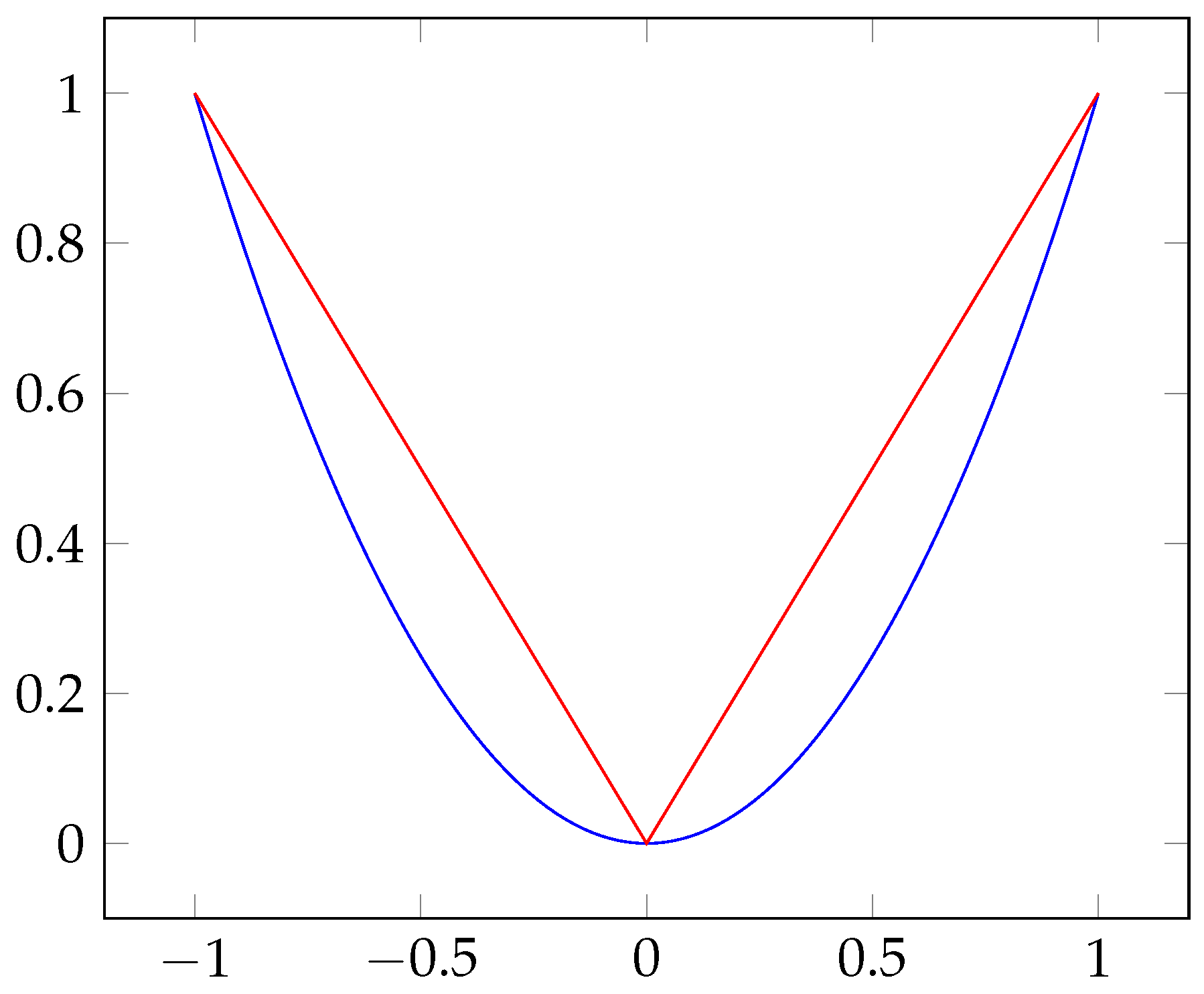
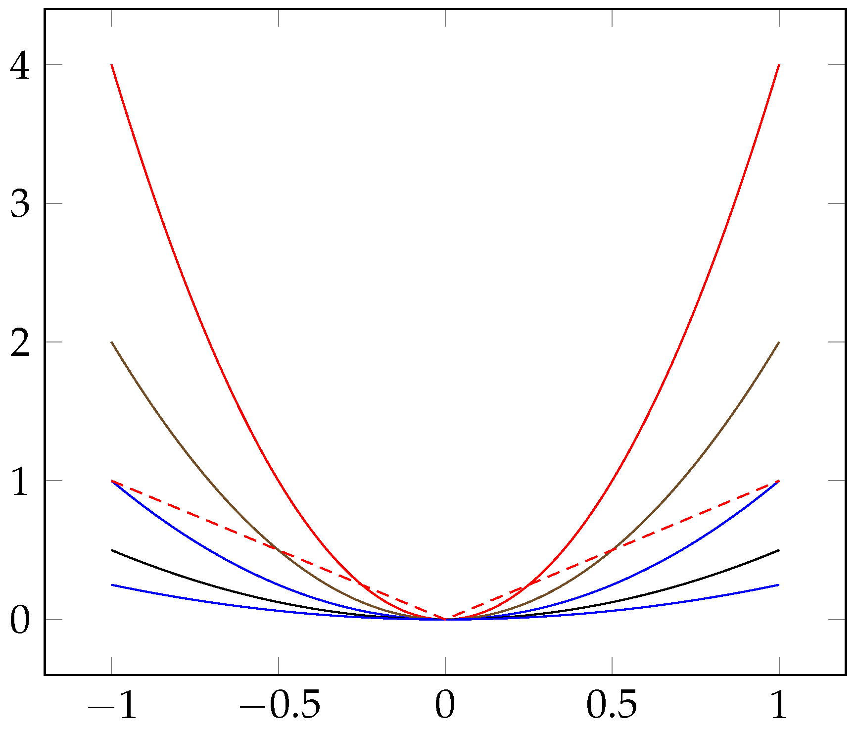
Now, with respect to Figure 2 and Figure 3, the intuitive and geometrical base for drawing a one-to-one function between the $L_1$ and $L_2$ penalties is possible (each imaginary line drawn parallel to the vertical axis only touches one point of the graphs of $L_1$ and $L_2$), whereas the graph of elastic-net is settled somewhere between the $L_1$ and $L_2$ penalties with the properties of being monotonic and invertable, so the rule of one-to-one function is still valid [29,35]. In other words, the elastic-net penalty function regarding the definition of its penalty function ($\lambda \left[{(1-\alpha )\left|\beta \right|}^2+\alpha {\left|\beta \right|}_1\right]$) has responses for its unknown coefficients.

Now, based on explanation above, instead of using ${\lambda }_1$ and ${\lambda }_2$ in computations, we use only ${\lambda }_{new}$ via the development of our deep neural network algorithm. The simplicity of the procedure, which has roughly the same accuracy as using both individual ${\lambda }^{\prime }s$, and calculation speed, are two advantages of ${\lambda }_{new}$. And all the R codes are written step by step with respect to the mathematical development of the methods of the different DNNs based on the basic mathematics of them in the following, as well as in the appendix. The basic mathematics of DNNs are thoroughly provided in Appendix A.

It is time to examine the $L_2$ regularization technique at this point. We are aware that the primary goal of our model is to decrease the amount of the cost function, where the following is true:

$\mathrm{Cost}={\displaystyle \frac{1}{m}}{\sum }_{i=1}^m{\mathrm{Loss}}_i$, in which m is the number of observations in a dataset. If we add the term ${\sum }_{j=1}^n{\displaystyle \frac{\lambda }{2m}}{\left|W_j\right|}^2$ in our cost function, then it will create a nullifying effect of certain parameters. In fact, the additional term attempts to reduce the values of the cost function by requiring our model to change (lower) the value of weights, $W^{\prime }s$, as well. As a result, some of the $W^{\prime }s$ carry out the nullification process since they are close to zero. Here, $\lambda$, as a regularization parameter or tuner finds tunes and can be considered as the proportion of linearity and non-linearity in our model. Therefore, increasing the value of $\lambda$ will force our model to reduce the value of $W^{\prime }s$ even more, and so it increases the linearity even more. Now, if we replace the modulus of $W^{\prime }s$ in the penalty term of the cost function, we will have $L_1$ regularization as

$$\mathrm{Cost}={\displaystyle \frac{1}{m}}\sum _{i=1}^m{\mathrm{Loss}}_i+\sum _{l=1}\sum _{i=1}\sum _{j=1}{\displaystyle \frac{\lambda }{2m}}\left|W_j\right|,$$

Again, this added term will force some $W^{\prime }s$ to tend to 0. So, we can write a general equation for a regularized DNN as below:

$$\mathrm{Cost}={\displaystyle \frac{1}{m}}\sum _{i=1}^m{\mathrm{Loss}}_i+\sum _{l=1}^L\sum _{i=1}^m\sum _{j=1}^n{\displaystyle \frac{\lambda }{2m}}{\left|W_{ij}^{\left[l\right]}\right|}^2,$$

(4)

where m is the number of observations, n is the number of dimensions, and l is related to the number of layers. The $\mathit{W}$ matrix for any $\left(l^{th}\right)$ layer can be considered as follows:

$$W^{\left[l\right]}=\left(\begin{array}{cccc}{w}_{11}^{\left[l\right]}& w_{12}^{\left[l\right]}& \dots & w_{1n}^{\left[l\right]}\\ w_{21}^{\left[l\right]}& w_{22}^{\left[l\right]}& \dots & w_{2n}^{\left[l\right]}\\ ⋮& ⋮& \ddots & ⋮\\ w_{m1}^{\left[l\right]}& w_{m2}^{\left[l\right]}& \dots & w_{mn}^{\left[l\right]}\end{array}\right),$$

(5)

Then, we have to calculate:

$$\sum W^2={\left(w_{11}^{\left[l\right]}\right)}^2+{\left(w_{12}^{\left[l\right]}\right)}^2+\cdots +{\left(w_{21}^{\left[l\right]}\right)}^2+{\left(w_{22}^{\left[l\right]}\right)}^2+\cdots +{\left(w_{m1}^{\left[l\right]}\right)}^{+}{\left(w_{m2}^{\left[l\right]}\right)}^{+}\cdots +{\left(w_{mn}^{\left[l\right]}\right)}^2.$$

(6)

It is worth noting that if we are adding any term to our cost function, we will also need to change our back-propagation equations. Because, in the back-propagation algorithms, we definitely face with ${\displaystyle \frac{\partial \mathrm{Cost}}{\partial W}}$ and so when we calculate ${\displaystyle \frac{\partial \mathrm{Cost}}{\partial W}}$, it is also needed to add the derivative of this term ${\sum }_{l=1}^L{\sum }_{i=1}{\sum }_{j=1}{\displaystyle \frac{\lambda }{2m}}{\left|W_{ij}^{\left[l\right]}\right|}^2.$ The derivative ${\displaystyle \frac{\partial \sum W^2}{\partial w_{ij}^{\left[l\right]}}}$ of Equation (9) is equal to $(2\times w_{ij})$, because the rest of weights except $w_{ij}$, are considered as constant values. Thus, the entire derivative of this term ${\sum }_{l=1}^L{\sum }_{i=1}{\sum }_{j=1}{\displaystyle \frac{\lambda }{2m}}{\left|W_{ij}^{\left[l\right]}\right|}^2$ is going to be ${\displaystyle \frac{\lambda }{m}}\times W^{\left[l\right]},$ where $\left(W^{\left[l\right]}\right)$ is a matrix containing all the weight parameters of that layer.

2.3. Constructing Two Heuristics DNN Approaches Based on the Shrinkage Penalized Methods

In Section 2.2, we illustrated how we employ the idea of an elastic-net penalty function in the GLMs in order to develop the algorithms of DDN. We have created two heuristic approaches for DNN based on practical statistical evidence, including current shrinkage penalized methods such as the combination of ridge and Lasso (elastic-net) and ridge&bridge. We defined a new penalty term in the structure of DNN with respect to the restrictions of any hyper-parameters in the penalized equation of the elastic-net. The important issue is that we have to consider that the coefficients, $\left({\beta }^{\prime }s\right)$, in the GLM’s penalty terms are somehow the weights, $\left(W^{\prime }s\right)$, in the structure of the DNN. Additionally, while describing the function of cost in DNNs, it is required to embed them in the back-propagation section in addition to including the penalty term in the cost function.

Now, in order to introduce an extension of the DNN’s algorithm and generalize its shrinkage penalized structures in other circumstances, such as the ${\mathrm{DNN}}_{\mathrm{elastic-net}}$ and ${\mathrm{DNN}}_{\mathrm{ridge} \& \mathrm{bridge}}$ we need to develop Equation (5) and prepare it for usage with variously developed DNN’s algorithms. In this regard, the general form of the elastic-net (en) cost function is defined as below:

$${\mathrm{Cost}}_{en}={\displaystyle \frac{1}{m}}\sum _{i=1}^m{\mathrm{Loss}}_i+\sum _{l=1}^L\sum _{i=1}^m\sum _{j=1}^n\lambda \left[{\displaystyle \frac{(1-\alpha )}{2m}}{\left(W_{ij}\right)}^2+{\displaystyle \frac{\alpha }{m}}\left|W_{ij}\right|\right],$$

(7)

where m is the number of observations, n is the number of dimensions, l is the number of layers, $\lambda >0$ is the size of penalty or tuning parameter, and $\alpha$ determines the type of penalty in the DNN’s structure, $(\alpha \in [0,1\left]\right)$. It is revealed that $(\alpha =0)$ is equivalent to the $L_2$ regularization and $(\alpha =1)$ is equivalent to the $L_1$ regularization. Therefore, the derivation of the elastic-net cost function must be calculated and then embedded in the back-propagation section to examine the effects of the regularization term that has been added. Similarly to the calculated derivations of the cost functions in Section 2.2, the derivation $\left({\displaystyle \frac{\partial \mathrm{Cost-en}}{\partial W}}\right)$ can be written as:

$${\displaystyle \frac{\partial {\mathrm{Cost}}_{en}}{\partial W}}={\displaystyle \frac{\lambda (1-\alpha )}{2m}}\times 2\times W_{ij}+{\displaystyle \frac{\lambda \alpha }{m}}\times {\displaystyle \frac{W_{ij}}{|W_{ij}|}}.$$

(8)

So, we can extend the regularization term to elastic-net.

We have now reached the final stage of the DNN regularization process, which is based on the elastic-net structure and represents one example of the general “ridge&bridge” regularization in GLMs. With respect to Equations (5) and (6), the elastic-net cost function in general is defined as below:

$${\mathrm{Cost}}_{Enet}={\displaystyle \frac{1}{m}}\sum _{i=1}^m{\mathrm{Loss}}_i+\sum _{l=1}^L\sum _{i=1}^m\sum _{j=1}^n\lambda \left[{\displaystyle \frac{(1-\alpha )}{2m}}{\left(W_{ij}\right)}^2+{\displaystyle \frac{\alpha }{m}}{\left|W_{ij}\right|}^{\gamma }\right],$$

(9)

where the restriction of $\left(\gamma \right)$ determines different types of ridge&bridge shrinkage regularizations in DNN structures, $(\gamma >0\mathrm{and}\gamma \ne 2)$. The derivation of the cost function of Equation (A23) with respect to the weights can be written as follows:

$${\displaystyle \frac{\partial {\mathrm{Cost}}_{Enet}}{\partial W}}={\displaystyle \frac{\lambda (1-\alpha )}{2m}}\times 2\times W_{ij}+{\displaystyle \frac{\lambda \alpha \gamma }{m}}\times {\displaystyle \frac{W_{ij}}{|W_{ij}|}}\times {\left|W_{ij}\right|}^{\gamma -1}.$$

(10)

By using Equation (10) in the cost function of the shrinkage-regularized DNN structure and embedding Equation (A1) in the back-propagation section of it, we developed and generalized the shrinkage penalization algorithm of DDN. Based on this development and generalization, we can present a wide range of penalized DNN models that take advantage of the general GLM penalization.

3. Microbiome Data

Operational Taxonomic Units (OTUs) are the basic unit used in numerical taxonomy. A typical microbiome dataset has thousands of OTUs and a small number of samples. These units may refer to an individual, species, genus, or class. The taxonomic units utilized in numerical approaches are invariably not equivalent to the formal taxonomic units [36,37]. Much of the challenge in analyzing microbiome data stems from the fact that they involve, either explicitly or implicitly, quantities of a relational nature. As such, measurements are typically both high-dimensional and dependent. Additionally, such data are often substantial in quantity, and thus computational tractability is generally an issue not far from the surface when developing and using statistical methods and models in this area. High dimensionality, non-normal distribution, and spurious correlation, among others, even make non-parametric methods invalid, and hence, analysis and interpretation of microbiome phenomena are very problematic [38,39].

Typically, there are four general characteristics of microbiome data. First of all, they are compositional, which means that the sum of the percentage of all bacteria in each sample is equal to or almost equal to 1. Secondly, the microbiome datasets are high-dimensional. Third, they are overdispersed, meaning that their variances are much larger than their means. Finally, often microbiome datasets are sparse with many zeros. So, for these couple of unique characteristics, the analysis of microbiome datasets is very challenging [40].

3.1. Simulation Study for Microbiome Data

In this sub-section, we individually particularized the equation of an elastic-net for the penalized logistic regression model. This particularization is important since employing Algorithm 1 will make the calculation and programming easier when implementing the model. As is well known, a binary logistic regression model is used to model the probability of certain events [41]. In the case of a binary response variable, the linear relationship between the predictor variables $\mathit{X}$ and response variable $\mathit{y}$ is explained by a logit model. Note that a logistic regression model with $\pi ({\mathit{x}}_i;\mathit{\beta })=P(Y_i=1|{\mathit{x}}_i)$ is explained by:

$$\begin{array}{cc}\hfill \log \left({\displaystyle \frac{\pi ({\mathit{x}}_i;\mathit{\beta })}{1-\pi ({\mathit{x}}_i;\mathit{\beta })}}\right)& ={\beta }_0+\sum _{j=1}^p{x}_{ij}{\beta }_j+{ϵ}_i,\hfill \end{array}$$

where ${\mathit{x}}_i={(x_{i1},\dots ,x_{ip})}^T\in {\mathbb{R}}^p$ is considered as the predictor variable, $\mathit{\beta }={({\beta }_0,{\beta }_1,\dots ,{\beta }_p)}^T$$\in {\mathbb{R}}^{p+1}$ is an unknown regression coefficient, and $y_i$ denotes a binary response variable with parameter $\pi ({\mathit{x}}_i;\mathit{\beta })$. Based on the [12], the log-likelihood of the penalized logistic regression model with the elastic-net penalty can be written as follows:

$$\begin{array}{cc}\hfill ł{\left(\mathit{\beta }\right|\mathit{y},\mathit{X})}_{\alpha ,\lambda }^{Enet}& =\sum _{i=1}^n\left[y_i\log \pi ({\mathit{x}}_i;\mathit{\beta })+(1-y_i)\log (1-\pi ({\mathit{x}}_i;\mathit{\beta }))\right]\hfill \\ & -{\displaystyle \frac{1}{2}}{\mathit{\beta }}^T{\mathit{Q}}_{{\lambda }_1}\mathit{\beta }-{\displaystyle \frac{1}{2}}{\mathit{\beta }}^T{\mathit{Q}}_{{\lambda }_2}\mathit{\beta }.\hfill \end{array}$$

Algorithm 1 Extendable algorithm of the neural network.

1: Initialize weights randomly. 2: Forward propagation w.r.t. the suitable increased hidden layers. 3: Find the value of cost function. 4: Backward propagation. 5: Repeat Steps 2, 3 and 4, many times until to reach minimum cost function.

Since the microbiome simulation scenario is a little complex and requires a lot of steps to generate simulated microbiome data, we just put references that we have used them [40,42,43]. The method used to deal with zeros in compositional data is an important step in the preparation of the simulated microbiome dataset [44,45,46,47]. We used the “zCompositions” package in R 4.1.1 software to solve the zero problem.

We could generate “compositional high-dimensional simulated microbiome dataset” with the property of normal distribution. But apparently, the actual microbiome dataset has no response or a “$y$” variable. So, based on the nature of microbiome datasets, we can extract the response variable from it (extracting hidden response variable) [38,39]. In clinical studies, usually the natural effect of the microbiome can determine different opposite cases, such as high/low or healthy/disease; hence, we defined two clusters for them. We applied the “Ward-D2” clustering algorithm over the incomplete real microbiome dataset and binned the results of clustering (0/1) as a dependent variable, “$y$”, to the dataset (we used the same process for generating the simulated one). In this study, in order to evaluate the developed algorithm, a simulated dataset with $n=200$ observations for $p=4000$ dimensions (explanatory variables) was generated. The simulated dataset was organized to have binary response variables ($0|1$ or $\mathrm{yes}\left|\mathrm{no}\right)$. With regard to the nature of microbiome data, we now put all of the aforementioned strategies into practice to generate compositional, high-dimensional data.

The simulation has 200 (150 + 50) observations for 4000 dimensions, which is carried out as below:

Class $\left(\mathit{I}\right).$ The first category of the second simulated dataset has $n=150$ observations for $p=4000:(2500\mathrm{Poisson}\mathrm{with}\lambda =2)+(50\mathrm{Poisson}\mathrm{with}\lambda =80)+(1450\mathrm{Poisson}\mathrm{with}\lambda =2)$ dimensions, ${\mathit{\beta }}_{\mathrm{class}\mathit{I}}\sim u(0.05,0.15)$ and the correlation structures ∼$u(0.75,0.95)$, ∼$u(0.5,0.95)$, and ∼$u(0.75,0.95)$, respectively.

Class $\left(\mathit{II}\right).$ The second category of the second simulated dataset is included $n=50$ observation for $p=4000:(2000\mathrm{Poisson}\mathrm{with}\lambda =2)+(100\mathrm{Poisson}\mathrm{with}\lambda =100)+(1900\mathrm{Poisson}\mathrm{with}\lambda =2)$ dimensions, ${\mathit{\beta }}_{\mathrm{class}\mathit{II}}=\mathbf{0}$ and the correlation structures: ∼$u(0.75,0.95)$, ∼$u(0.5,0.95)$, and ∼$u(0.75,0.95)$, respectively.

Every Poisson distribution parameter, $\lambda$, has been assigned randomly. The Aitchison transformation method will then be used to normalize each of these non-normal simulated datasets. After that, the simulated data was fed into the general and penalized DNN using the methodology outlined for the development of the penalized DNN model. Namely, five DNN models were generated: ${\mathrm{DNN}}_{\mathrm{general}}$, ${\mathrm{DNN}}_{\mathrm{ridge}}$, ${\mathrm{DNN}}_{\mathrm{Lasso}}$, ${\mathrm{DNN}}_{\mathrm{elastic-net}}$, and ${\mathrm{DNN}}_{\mathrm{ridge}\&\mathrm{bridge}}$. This is repeated on 30 training and testing datasets. All penalized DNNs are evaluated by taking the mean of the following performance metrics: prediction accuracy and sensitivity, together with their confidence intervals (see

Table 1. Simulated compositional high-dimensional data $(n=200,p=4000)$. The division of training and testing data are $70\%$ and $30\%$, respectively. The baselines for the new shrinkage penalized approaches (${\mathrm{DNN}}_{\mathrm{elastic-net}}$ and ${\mathrm{DNN}}_{\mathrm{ridge}\&\mathrm{bridge}}$) are (${\mathrm{DNN}}_{\mathrm{ridge}}$ and ${\mathrm{DNN}}_{\mathrm{Lasso}})$.

Type of the Deep Neural Network Model	Prediction Accuracy of Whole Dataset (%), Mean [CI 95%]	Sensitivity of Whole Dataset (%), Mean [CI 95%]	Prediction Accuracy of Training Dataset (%), Mean [CI 95%]	Sensitivity of Training Dataset (%), Mean [CI 95%]	Prediction Accuracy of Testing Dataset (%), Mean [CI 95%]	Sensitivity of Testing Dataset (%), Mean [CI 95%]
${\mathrm{DNN}}_{\mathrm{general}}$	80	$78.9$	$79.2$	$78.2$	$82.8$	$81.5$
	$[79.77,80.23]$	$[78.53,79.27]$	$[78.77,79.63]$	$[77.64,78.76]$	$[82.46,83.14]$	$[80.86,82.14]$
${\mathrm{DNN}}_{\mathrm{ridge}}$	$82.5$	$81.9$	$80.8$	$79\%$	$83.8$	$83.4$
	$[81.78,83.22]$	$[81.22,82.58]$	$[80.09,81.51]$	$[78.52,79.48]$	$[83.03,84.57]$	$[82.74,84.06]$
${\mathrm{DNN}}_{\mathrm{Lasso}}$	82	$81.5$	80	$78.3$	$82.9$	$82.4$
	$[81.19,82.81]$	$[80.57,82.43]$	$[79.17,80.73]$	$[77.61,78.99]$	$[81.99,83.81]$	$[81.57,83.23]$
${\mathrm{DNN}}_{\mathrm{elastic-net}}$	$84.2$	$83.5$	82	$80.8$	$83.9$	$83.4$
	$[83.37,85.03]$	$[82.49,84.51]$	$[81.18,82.88]$	$[79.93,81.67]$	$[82.93,84.87]$	$[82.51,84.29]$
${\mathrm{DNN}}_{\mathrm{ridge}\&\mathrm{bridge}}$	84	$83.3$	$81.8$	$80.3$	$83.6$	$82.9$
	$[82.88,85.12]$	$[82.45,84.15]$	$[81.09,82.51]$	$[79.37,81.23]$	$[82.37,84.83]$	$[81.94,83.86]$
GUIDE	81	82	$80.2$	$79.6$	$80.8$	$80.2$
	$[80.21,81.79]$	$[81.14,82.86]$	$[79.43,80.97]$	$[78.71,80.49]$	$[79.97,81.63]$	$[79.75,80.65]$

The performance of the ${\mathrm{DNN}}_{\mathrm{general}}$, ${\mathrm{DNN}}_{\mathrm{ridge}}$, ${\mathrm{DNN}}_{\mathrm{Lasso}}$, ${\mathrm{DNN}}_{\mathrm{elastic-net}}$, ${\mathrm{DNN}}_{\mathrm{ridge}\&\mathrm{bridge}}$, and classification tree with the GUIDE method. The performance measures included are the average prediction accuracy, the average sensitivity, and the confidence interval for the average prediction accuracy and sensitivity. The prediction accuracy is calculated based on the following formula. Accuracy: ${\displaystyle \frac{\mathrm{TP}+\mathrm{TN}}{\mathrm{TP}+\mathrm{TN}+\mathrm{FP}+\mathrm{FN}}}$ where TP is the abbreviation of True Positive, TN is the abbreviation of True Negative, FP is the abbreviation of False Positive, and FN is the abbreviation of False Negative. The sensitivity is calculated based on the following formula: Sensitivity = ${\displaystyle \frac{\mathrm{TP}}{\mathrm{TP}+\mathrm{FN}}}$. This is repeated 30 times on the whole, training, and testing datasets.

and

Table 2. Real compositional high-dimensional data $(n=675,p=6696)$. The baselines for the new shrinkage penalized approaches (${\mathrm{DNN}}_{\mathrm{elastic-net}}$ and ${\mathrm{DNN}}_{\mathrm{ridge}\&\mathrm{bridge}}$) are (${\mathrm{DNN}}_{\mathrm{ridge}}$ and ${\mathrm{DNN}}_{\mathrm{Lasso}})$.

Type of the Deep Neural Network Model	Prediction Accuracy of Whole Dataset, %	Sensitivity of Whole Dataset, %	Prediction Accuracy of Training Dataset %, Mean [CI 95 %]	Sensitivity of Training Dataset %, Mean [CI 95 %]	Prediction Accuracy of Testing Dataset %, Mean [CI 95 %]	Sensitivity of Testing Dataset %, Mean [CI 95 %]
${\mathrm{DNN}}_{\mathrm{general}}$	$90.1\%$	$90.1\%$	$90.7\%$	$90.9\%$	$89.2\%$	$89.1\%$
			$[89.77,91.63]$	$[89.98,91.82]$	$[88.33,90.07]$	$[88.33,89.87]$
${\mathrm{DNN}}_{\mathrm{ridge}}$	$90.5\%$	$90.5\%$	$91.9\%$	$92.6\%$	$90.3\%$	$90.6\%$
			$[90.83,92.93]$	$[91.46,93.74]$	$[89.41,91.19]$	$[89.83,91.37]$
${\mathrm{DNN}}_{\mathrm{Lasso}}$	$90.1\%$	$90.1\%$	$91.1\%$	$91.2\%$	$90.3\%$	$90.6\%$
			$[90.11,92.09]$	$[90.38,92.08]$	$[89.39,91.21]$	$[89.71,91.49]$
${\mathrm{DNN}}_{\mathrm{elastic-net}}$	$93.6\%$	$94.8\%$	$93.4\%$	$93.5\%$	$92.3\%$	$92.6\%$
			$[92.06,94.74]$	$[92.28,94.72]$	$[91.33,93.27]$	$[91.79,93.41]$
${\mathrm{DNN}}_{\mathrm{ridge}\&\mathrm{bridge}}$	$92.1\%$	$92.7\%$	$92.9\%$	$93.2\%$	$91.9\%$	$92.2\%$
			$[91.97,93.83]$	$[92.11,94.29]$	$[91.01,92.79]$	$[91.33,93.07]$
GUIDE	$89\%$	$91.4\%$	$89.2\%$	$91.6\%$	$89.1\%$	$91.4\%$
			$[88.41,89.99]$	$[90.57,92.63]$	$[88.19,90.92]$	$[90.43,92.37]$

The performance of the ${\mathrm{DNN}}_{\mathrm{general}}$, ${\mathrm{DNN}}_{\mathrm{ridge}}$, ${\mathrm{DNN}}_{\mathrm{Lasso}}$, ${\mathrm{DNN}}_{\mathrm{elastic-net}}$, ${\mathrm{DNN}}_{\mathrm{ridge}\&\mathrm{bridge}}$, and classification tree with the GUIDE method. The performance measures included are the average prediction accuracy, the average sensitivity, and the confidence interval for the average prediction accuracy and sensitivity. The prediction accuracy is calculated based on the following formula. Accuracy: ${\displaystyle \frac{\mathrm{TP}+\mathrm{TN}}{\mathrm{TP}+\mathrm{TN}+\mathrm{FP}+\mathrm{FN}}}$ where TP is the abbreviation of True Positive, TN is the abbreviation of True Negative, FP is the abbreviation of False Positive, and FN is abbreviation of False Negative. The sensitivity is calculated based on this formula: Sensitivity = ${\displaystyle \frac{\mathrm{TP}}{\mathrm{TP}+\mathrm{FN}}}$. This is repeated 30 times on the whole, training, and testing datasets.

).

3.2. Classification of Simulated Microbiome Data Based on the Elastic-Net Penalization Using DNN

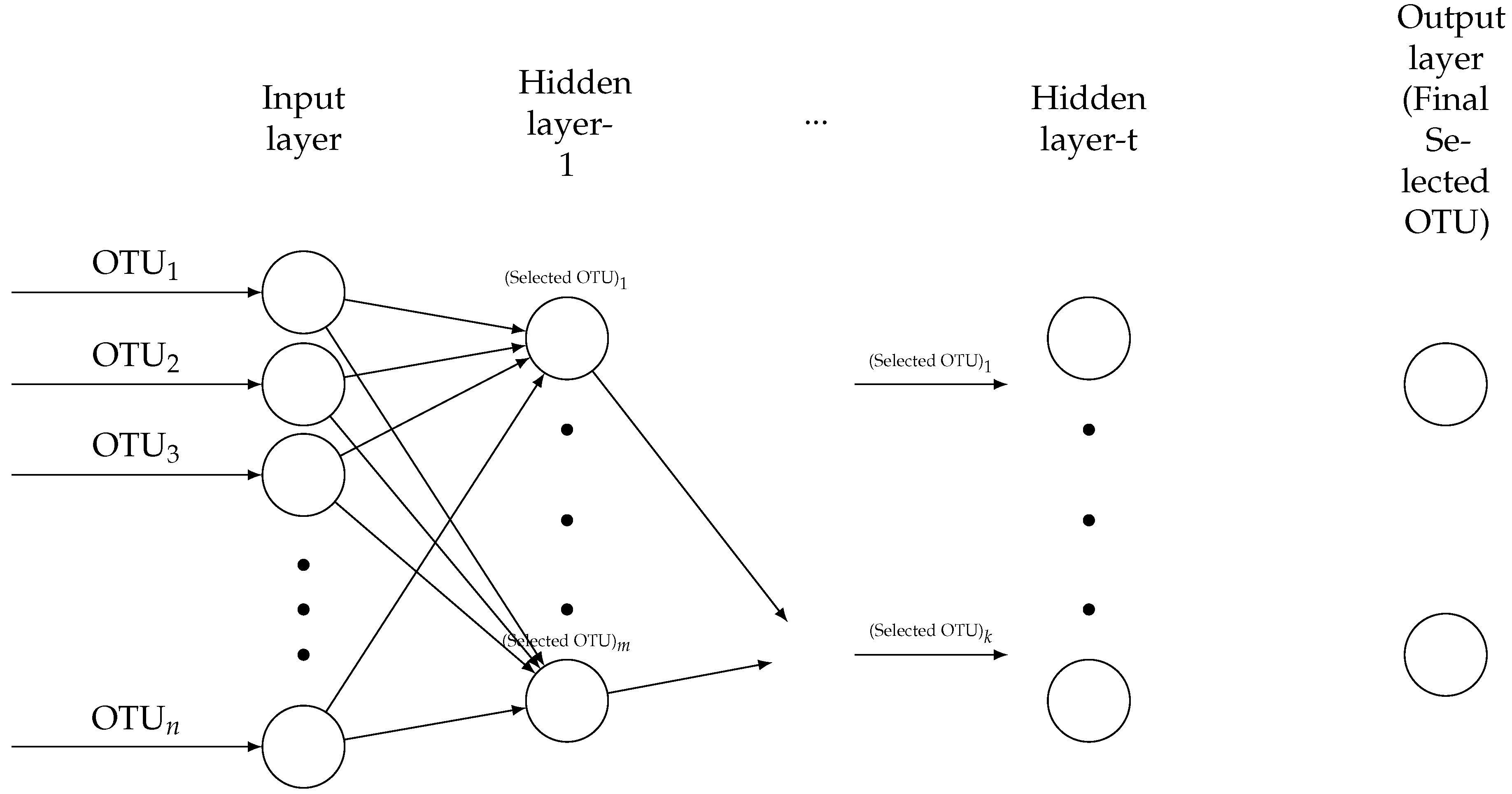
In Section 3.2, we classified one kind of compositional high-dimensional simulated data called microbiome data for 200 observations and 4000 dimensions. In general, Figure 4 and Figure 5 show the data-transferring process inside a deep neural network algorithm in use as well as the fundamental mother role for this algorithm. We can state concisely that the simulated OTU data are first placed in the input vector. After applying numerous processes to the data, the findings are eventually extracted. The results of different types of the elastic-net, such as ridge $(\alpha =0)$, Lasso $(\alpha =1,\gamma =1)$, elastic-net $(\alpha \ne 1,\gamma =1)$ and bridge $(\alpha =1)$, in our developed DNN are illustrated in Table 1 (also see [12]), whereas the general DNN algorithm is developed based on different regularization methods; hence, for each desired model, the related penalized hyperparameters such as $\alpha$, $\lambda$ and $\gamma$ are added to their penalty functions. Therefore, as with the parametric regularization method for classification, the different values of hyperparameters have their own effect on the DNN-penalized prediction accuracy as a non-parametric method for classification.

Now, with respect to the previous paragraph, we can more clearly explain Table 1. As observed in Table 1, aside from the general DNN, there are four penalized DNN models, such as ${\mathrm{DNN}}_{\mathrm{ridge}}$, ${\mathrm{DNN}}_{\mathrm{Lasso}}$, ${\mathrm{DNN}}_{\mathrm{elastic-net}}$, and ${\mathrm{DNN}}_{\mathrm{ridge}\&\mathrm{bridge}}$. Additionally, we employed GUIDE as a second non-parametric binary classifier to have a strong rival when comparing its outcomes to those of general and penalized binary DNNs. In order to perform these methods, we first applied all available DNNs to the entire simulated dataset. Next, we divided the simulated dataset into training $(70\%)$ and testing $(30\%)$ datasets. Prediction of model accuracy and model sensitivity are the evaluation criteria for the proposed approaches. In Table 1, besides the general DNN model, the prediction accuracy, sensitivity, and amount of cost function for the whole, training, and testing simulated datasets are listed for each type of penalized DNN model. As seen in Table 1, across all training and testing simulated datasets, the overall prediction accuracy of penalized DNNs is higher than the general DNN model.

The ${\mathrm{DNN}}_{\mathrm{elastic-net}}$ has more prediction accuracy and sensitivity than the general and other penalized DNNs among the whole dataset. As observed in Table 1, in the whole dataset, the ${\mathrm{DNN}}_{\mathrm{ridge}\&\mathrm{bridge}}$, ${\mathrm{DNN}}_{\mathrm{ridge}}$, ${\mathrm{DNN}}_{\mathrm{Lasso}}$, and ${\mathrm{DNN}}_{\mathrm{general}}$ have the next most prediction accuracy and sensitivity DNNs, respectively.

In the training simulated OTU dataset, again, the prediction accuracy and sensitivity of the ${\mathrm{DNN}}_{\mathrm{elastic-net}}$ are larger than the general and other penalized DNN models, $82\%$ and $80.8\%$, respectively. The general DNN has the lowest prediction accuracy among all penalized models for the training dataset, $79.2\%$. In contrast to the whole and testing dataset, in the training dataset, the values of prediction accuracy and sensitivity of DNNs have slightly decreased, but the order of prediction, accuracy, and sensitivity of DNNs is the same as the whole dataset.

In the testing simulated OTU dataset, the trend of growth in the prediction accuracy and sensitivity is not exactly similar to the order of them in the whole and training datasets. For instance, ${\mathrm{DNN}}_{\mathrm{ridge}}$ has more prediction accuracy and sensitivity $(83.8\%\mathrm{and}83.4\%)$ than ${\mathrm{DNN}}_{\mathrm{ridge}\&\mathrm{bridge}}$$(83.6\%\mathrm{and}82.9\%)$. One reason might be the type of dataset that is compositional (OTU data), and another reason might be the reduction in the number of observations in the testing dataset. ${\mathrm{DNN}}_{\mathrm{elastic-net}}$ has the highest values of prediction accuracy and sensitivity $83.9\%\mathrm{and}83.4\%$, respectively. As observed, the general DNN algorithm for testing simulated OTU data has the lowest prediction accuracy and sensitivity in comparison with other penalized DNN models.

The last column of Table 1 shows the amount of the cost function for both the general and penalized DNN algorithms in terms of decreasing or increasing. We see that the values of prediction accuracy and sensitivity can be larger, but at the expense of increasing the cost function in the algorithm. So, during the implementation process, if the cost function is not so big, then to increase the model accuracy and sensitivity (and maybe other desired criteria), all of the regularization processes in the penalized DNN models can be employed. The results of implementation of the GUIDE method over the same simulated OTU data (whole, training, and testing simulated OTU data) were shown in Table 1 as well. As seen, there is stiff competition between the algorithms of the DNNs and GUIDE based on different criteria. It is worth noting that GUIDE has a larger prediction accuracy in comparison with the general DNN by employing the whole and training datasets. However, the prediction accuracy of all penalized DNNs is higher than GUIDE, but the sensitivity of GUIDE in the whole and training datasets is larger than some DNN algorithms such as ${\mathrm{DNN}}_{\mathrm{general}}$, ${\mathrm{DNN}}_{\mathrm{ridge}}$, and ${\mathrm{DNN}}_{\mathrm{Lasso}}$. The prediction accuracy and sensitivity of GUIDE are less than DNNs in testing datasets.

3.3. Classification of Simulated Microbiome Data with GUIDE

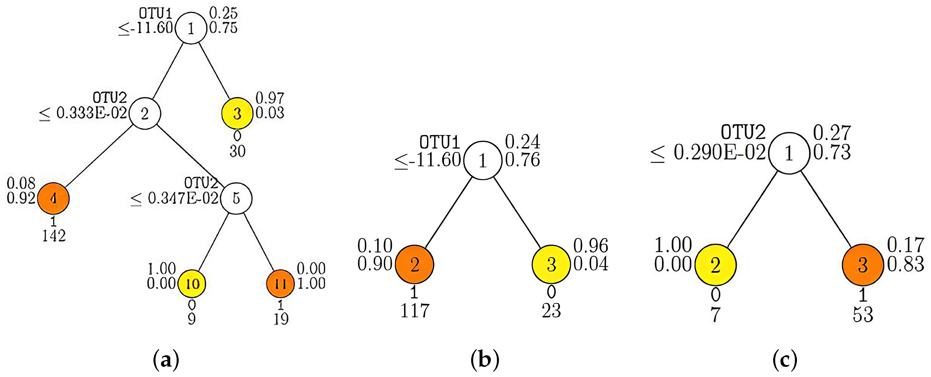
GUIDE is an algorithm for the construction of classification and regression trees and forests [48,49]. As we know, the predictors, $\mathit{x}$, are combined in a linear scheme to represent the effect on the response in the linear model. Sometimes, greater flexibility is needed since this linearity is insufficient to reflect the structure of the data. Because it combines the predictors in a non-parametric way, the models like additive models, trees, and neural networks enable them to fit a more flexible model of the response on predictors than the linear techniques [48]. In this study, we applied the GUIDE algorithm across identical simulated microbiome and real microbiome datasets in order to have a strong competitor for our proposed non-parametric method, i.e., penalizing various DNN models. Figure 6 shows how the GUIDE algorithm is applied to the whole training and testing datasets of simulated microbiome data, which are, respectively, indexed by (a), (b), and (c). The number of dimensions is 4000, and the number of observations for the whole, training, and testing datasets are 200, 140, and 60, respectively.

Based on the results of Table 1, it can be found that there is a stiff competition for prediction accuracy and sensitivity between developed penalized DNN models. In the implementation of penalized DNNs on the whole simulated dataset, the ${\mathrm{DNN}}_{\mathrm{elastic-net}}$ model has the highest prediction accuracy $(84.2\%)$. The same implementation using GUIDE on the whole dataset gives $81\%$ prediction accuracy. The same trend is observed for the training and testing simulated OTU dataset in both approaches, penalized DNNs and GUIDE. For instance, the ${\mathrm{DNN}}_{\mathrm{elastic-net}}$ has more accuracy in comparison with other penalized DNN models. As seen via Table 1, all the penalized DNN models have larger accuracy than the general DNN model.

We are now dealing with the GUIDE results for these simulated OTU data. For the whole, training, and testing simulated OTU dataset, Figure 6 shows three possible OTUs splitting by GUIDE. Note that GUIDE is applied pruning by k-fold cross-validation, with $k=10$, and the selected tree is based on the mean of CV estimates (the results of splitting have been summarized in Table 1). As can be found, the prediction accuracy of GUIDE for the whole simulated dataset is larger than its training and testing simulated datasets. It is important to notice that the GUIDE results fall between the created general DNN and penalized DNN models. The very interesting thing in Figure 6c is that the splitting is started by ${\mathrm{OTU}}_2$ while the splitting for the whole simulated dataset is started by ${\mathrm{OTU}}_1$. The reason for such changes is the starting point for splitting, which might be the decreasing number of sample sizes in the simulated testing dataset (see Figure 6a–c).

3.4. Classification of Real Microbiome Data Based on the Elastic-Net Penalization Using DNN

The performance of the applied penalized DNN models is demonstrated in this section using an actual compositional high-dimensional dataset, microbiome data, or OTU data (the source of the data can be found in [50]). A classification with the GUIDE method is then run on this dataset as a comparison. The applied OTU dataset includes 675 samples and 6696 different OTUs as predictors, which is considered a compositional ultra-high-dimensional case. As explained in Section 2, the development of the algorithm of the DNN based on a new penalization equation (the elastic-net equation) in fact enables us to apply the OTU data through different rival new penalized DNN models. Because there is no response variable in this OTU dataset, it must be created. So we may solve this early step challenge of the dataset using the OTU distance measurement attribute, which was described in Section 3.1 (also see [23,24]). In terms of the geometry of the OTU data, we must first move the data from simplex space to Euclidean space; after that, we must cluster the data into two sub-clusters. Finally, we can specify the response variables with regard to which of the two clusters they belong to. We can now test the binary classification of our built models using a new dataset that has binary responses. In summary, we created an ultra-high-dimensional compositional dataset using a variety of statistical techniques in order to create a binary response variable with respect to Section 3.1.

As mentioned, the focus of this research is related to the extension of the DNN using the “elastic-net” approach. Therefore, to display the property of various of the elastic-net penalties, such as ${\mathrm{DNN}}_{\mathrm{ridge}}$, ${\mathrm{DNN}}_{\mathrm{Lasso}}$, ${\mathrm{DNN}}_{\mathrm{elastic-net}}$, and ${\mathrm{DNN}}_{\mathrm{ridge}\&\mathrm{bridge}}$, different hyperparameters regarding the type of penalized DNN must be included in the DNN algorithm. Subsequently, the real OTU dataset is subjected to the expanded DNN algorithms. Additionally, a comparison is made with GUIDE. The evaluation results of various penalized DNN models are displayed in Table 2.

Table 2 shows that the general and penalized DNN models have been used over the whole training and testing datasets. The whole OTU dataset is divided into two parts: $70\%$ for training and $30\%$ for testing. The results of prediction accuracy and sensitivity in Table 2 for the whole dataset are almost similar to Table 1. Regarding Table 2, all of the penalized models plus the general DNN have the same prediction accuracy and sensitivity, with the exception of ${\mathrm{DNN}}_{\mathrm{elastic-net}}$ and ${\mathrm{DNN}}_{\mathrm{ridge}\&\mathrm{bridge}}$, which are the best DNN models, $93.6\%\mathrm{and}92.1\%$ for prediction accuracy and $94.8\%\mathrm{and}92.7\%$ for sensitivity, respectively. In terms of the prediction accuracy and sensitivity, the penalized DNN models show an improvement over the general DNN model up to $3.5\%$ in the training dataset. Although the results of the penalized DNN models for the training dataset demonstrate a fierce rivalry amongst them, the ${\mathrm{DNN}}_{\mathrm{elastic-net}}$ model predicts outcomes with the highest prediction accuracy and sensitivity when compared with the other regularized models, $93.4\%\mathrm{and}93.5\%$, respectively. Regarding sensitivity and prediction accuracy, Table 2 shows that all penalized DNN models produce better results for the testing dataset in comparison with the general DNN. As seen in Table 2, their performances are significantly superior to that of the general DNN model, $92.3\%\mathrm{vs}.89.2\%$ for prediction accuracy and $92.6\%\mathrm{vs}.89.1\%$ for model sensitivity (see the ${\mathrm{DNN}}_{\mathrm{general}}$ and ${\mathrm{DNN}}_{\mathrm{elastic-net}}$). The last column in Table 2 displays the cost function for both general and penalized DNN models for real OTU data with respect to the prediction accuracy and sensitivity (similar to the simulation study in Section 3.2).

The outcomes of the developed penalized DNN models were compared to the outcome of applying the same simulated dataset to the classification tree with the GUIDE method for evaluation purposes. The comparison results can be explained in two parts: the first part is included (GUIDE vs. general DNN), and the second part is included (GUIDE vs. penalized DNNs). In the first part, for the whole dataset, the general DNN outperforms GUIDE in terms of the prediction accuracy, $90.1\%$ vs. $89\%$, respectively, while GUIDE has greater sensitivity, $91.4\%$ vs. $90.1\%$. For training and testing datasets, the same trend is observable, although in different percentages (see Table 2). In the second part, penalized DNN methods make better predictions than classification trees with the GUIDE. However, GUIDE is slightly better than sensitivity in training datasets $\left({\mathrm{DNN}}_{\mathrm{Lasso}}\right)$ and testing datasets $\left({\mathrm{DNN}}_{\mathrm{ridge}}\right)$ and $\left({\mathrm{DNN}}_{\mathrm{Lasso}}\right)$ (see Table 2).

3.5. Classification of Real Microbiome Data with GUIDE

In Section 3.5, we first go over how data is prepared for the classification tree with the GUIDE method, and then we deal with the method outcomes. Preparing data for the GUIDE method is a challenging problem, particularly when dealing with high and ultra-high-dimensional datasets. In other words, making and preparing the appropriate datasets requires extreme precision in code writing in R software, then proper code writing for the GUIDE method. Code writing will be increasingly difficult as compositional high-dimensional collections become more complicated.

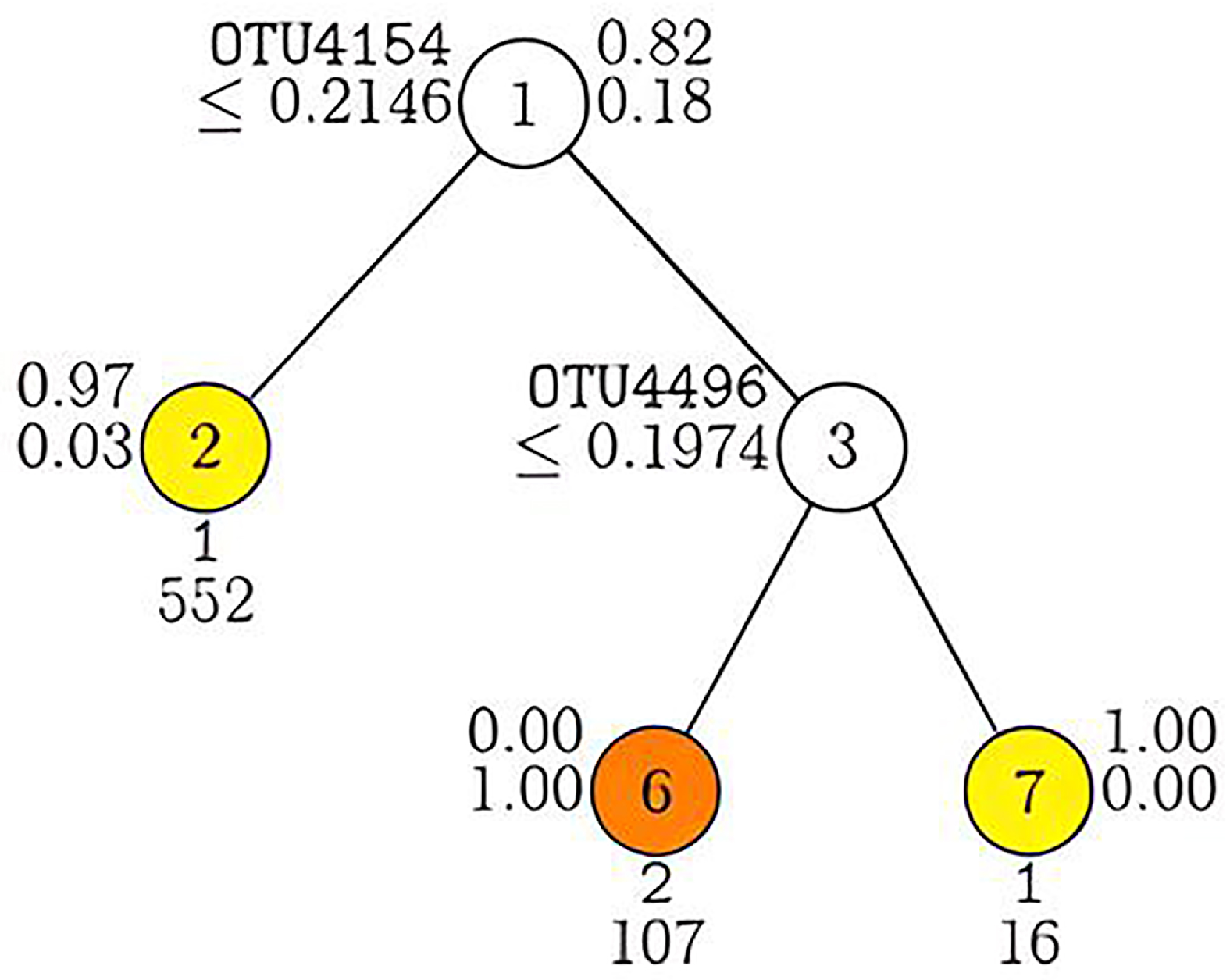
In order to achieve the best binary classification, Figure 7 illustrates which OUTs are highly significant and should be proposed for splitting the compositional high-dimensional dataset. The OTU indexed by 4154 is the best split variable for binary classification, as demonstrated among 6996 OTUs. Furthermore, it can be observed from Table 2 about the GUIDE classification tree outcomes for the actual dataset that this non-parametric approach can effectively rival the general DNN and its established penalized ones. Put differently, the classification tree with the GUIDE can be viewed as an assessment tool and a formidable competitor to our proprietary methods. Using the general DNN technique and the GUIDE findings in Table 2, we find that they are very competitive with each other for OTU dataset classification but not for developed penalized DNNs. Stated differently, two non-parametric approaches (the general DNN and GUIDE) nearly produce the identical results for both simulated and actual OTU datasets. It means that their ability for classification of OTU datasets is close to each other.

4. Conclusions and Future Works

In this paper, we developed a deep neural network method with respect to the notion of shrinkage GLM penalization strategies. Also, in this paper, the ratio of $L_1$ and $L_2$ norms has been used empirically as a criterion of combination of $L_1$ and $L_2$ to extend the concept and application of the DNNs. The elastic-net penalty, as a linear combination of ridge and bridge penalties, is a shrinkage regularization and penalization method for the elastic-net model. The curse of dimensionality and multicollinearity in large-scale datasets can be effectively addressed with the elastic-net technique. After understanding the idea behind the elastic-net technique, we attempted to apply it to the deep neural network algorithm determinative cores. Therefore, we increased the performance of the DNN algorithm in comparison with its general (classical) case. This improvement was confirmed through simulation and a real microbiome dataset via a non-parametric shrinkage penalized classification approach (shrinkage penalized DNN classification).

Furthermore, the outcomes of using a classification tree with the “GUIDE” method on the same simulated and real microbiome data are very competitive. The outcomes of a competition between two distinct non-parametric techniques (general and developed shrinkage penalized DNN models vs. the GUIDE method) show that the GUIDE method is extremely competitive with the general DNN. Still, as compared to the GUIDE, the classification results favor the developed shrinkage penalized DNN models. As a result, the researchers may choose a non-parametric scheme for their model building and prediction based on factors including time, budget, and required accuracy.

Many research titles can be proposed in relation to the conducted research: in order to generalize the findings and outcomes, more simulation and real-world studies on larger datasets (including and excluding compositional high-dimensional datasets) will be useful. Working on the some function of hyperparameters of the shrinkage penalized methods $(\alpha ,\lambda ,\mathrm{and}\gamma )$ in order to extend them in the DNN algorithm can be considered as a new interesting research (the shrinkage regularization process can include the generalization of hyperparameters), particularly developing the DNN algorithm’s theoretical foundations first and then its implementation. Also, further investigation into the implementation of ${\mathrm{DNN}}_{\mathrm{elastic-net}}$ and ${\mathrm{DNN}}_{\mathrm{ridge}\text{-}\&\mathrm{bridge}}$ models in comparison with ${\mathrm{DNN}}_{\mathrm{Lasso}}$ and ${\mathrm{DNN}}_{\mathrm{ridge}}$ penalties, with an eye toward (compositional) high-dimensional datasets, would be a worthwhile avenue for future research. Finally, examining the variation in cost functions across all versions of developed DNN models could be a future study focus.

References

1. Faraway, J.J. Extending the Linear Model with R: Generalized Linear, Mixed Effects and Nonparametric Regression Models; Chapman and Hall: New York, NY, USA, 2016. [Google Scholar]
2. Penrose, R. The emperor’s new mind: Concerning computers, minds, and the laws of physics. Behav. Brain Sci. 1990, 13, 643–655. [Google Scholar] [CrossRef]
3. Ciaburro, G.; Venkateswaran, B. Neural Networks with R: Smart Models Using CNN, RNN, Deep Learning, and Artificial Intelligence Principles; Packt Publishing Ltd.: Birmingham, UK, 2017. [Google Scholar]
4. Liu, Y.H.; Maldonado, P. R Deep Learning Projects: Master the Techniques to Design and Develop Neural Network Models in R; Packt Publishing Ltd.: Birmingham, UK, 2018. [Google Scholar]
5. Hornik, K.; Stinchcombe, M.; White, H. Multilayer feedforward networks are universal approximators. Neural Netw. 1989, 2, 359–366. [Google Scholar] [CrossRef]
6. Roozbeh, M.; Maanavi, M.; Mohamed, N.A. Penalized least squares optimization problem for high-dimensional data. Int. J. Nonlinear Anal. Appl. 2023, 14, 245–250. [Google Scholar]
7. De-Julián-Ortiz, J.V.; Pogliani, L.; Besalú, E. Modeling properties with artificial neural networks and multilinear least-squares regression: Advantages and drawbacks of the two methods. Appl. Sci. 2018, 8, 1094. [Google Scholar] [CrossRef]
8. Hammerstrom, D. Working with neural networks. IEEE Spectr. 1993, 30, 46–53. [Google Scholar] [CrossRef]
9. Salehin, I.; Kang, D.K. A review on dropout regularization approaches for deep neural networks within the scholarly domain. Electronics 2023, 12, 3106. [Google Scholar] [CrossRef]
10. Hertz, J.A. Introduction to the Theory of Neural Computation; Chapman and Hall: New York, NY, USA, 2018. [Google Scholar]
11. Fan, J.; Li, R. Statistical challenges with high dimensionality: Feature selection in knowledge discovery. arXiv 2006, arXiv:math/0602133. [Google Scholar]
12. Huang, J.; Breheny, P.; Lee, S.; Ma, S.; Zhang, C. The Mnet method for variable selection. Stat. Sin. 2016, 26, 903–923. [Google Scholar] [CrossRef]
13. Farrell, M.; Liang, T.; Misra, S. Deep neural networks for estimation and inference. Econometrica 2021, 89, 181–213. [Google Scholar] [CrossRef]
14. Kurisu, D.; Fukami, R.; Koike, Y. Adaptive deep learning for nonlinear time series models. Bernoulli 2025, 31, 240–270. [Google Scholar] [CrossRef]
15. Bach, F. Breaking the curse of dimensionality with convex neural networks. J. Mach. Learn. Res. 2017, 18, 1–53. [Google Scholar]
16. Celentano, L.; Basin, M.V. Optimal estimator design for LTI systems with bounded noises, disturbances, and nonlinearities. Circuits Syst. Signal Process. 2021, 40, 3266–3285. [Google Scholar] [CrossRef]
17. Liu, F.; Dadi, L.; Cevher, V. Learning with norm constrained, over-parameterized, two-layer neural networks. J. Mach. Learn. Res. 2024, 25, 1–42. [Google Scholar]
18. Shrestha, K.; Alsadoon, O.H.; Alsadoon, A.; Rashid, T.A.; Ali, R.S.; Prasad, P.W.C.; Jerew, O.D. A novel solution of an elastic net regularisation for dementia knowledge discovery using deep learning. J. Exp. Theor. Artif. Intell. 2023, 35, 807–829. [Google Scholar] [CrossRef]
19. Zhang, C.; Bengio, S.; Hardt, M.; Recht, B.; Vinyals, O. Understanding deep learning requires rethinking generalization. arXiv 2016, arXiv:1611.03530. [Google Scholar] [CrossRef]
20. Mulenga, M.; Kareem, S.A.; Sabri, A.Q.; Seera, M.; Govind, S.; Samudi, C.; Saharuddin, M.B. Feature extension of gut microbiome data for deep neural network-based colorectal cancer classification. IEEE Access 2021, 9, 23565–23578. [Google Scholar] [CrossRef]
21. Namkung, J. Machine learning methods for microbiome studies. J. Microbiol. 2020, 58, 206–216. [Google Scholar] [CrossRef]
22. Topçuoğlu, B.D.; Lesniak, N.A.; Ruffin, M.T.; Wiens, J.; Schloss, P.D. A framework for effective application of machine learning to microbiome-based classification problems. mBio 2020, 11, 10-1128. [Google Scholar] [CrossRef]
23. Anwar, S.M.; Majid, M.; Qayyum, A.; Awais, M.; Alnowami, M.; Khan, M.K. Medical image analysis using convolutional neural networks: A review. J. Med. Syst. 2018, 42, 226. [Google Scholar] [CrossRef]
24. Lo, C.; Marculescu, R. MetaNN: Accurate classification of host phenotypes from metagenomic data using neural networks. BMC Bioinform. 2019, 20, 314. [Google Scholar] [CrossRef]
25. Reiman, D.; Metwally, A.; Dai, Y. Using convolutional neural networks to explore the microbiome. In Proceedings of the 39th Annual International Conference of the IEEE Engineering in Medicine and Biology Society (EMBC), Jeju, Republic of Korea, 11–15 July 2017; pp. 4269–4272. [Google Scholar] [CrossRef]
26. Arabameri, A.; Asemani, D.; Teymourpour, P. Detection of colorectal carcinoma based on microbiota analysis using generalized regression neural networks and nonlinear feature selection. IEEE/ACM Trans. Comput. Biol. Bioinform. 2018, 17, 547–557. [Google Scholar] [CrossRef]
27. Fiannaca, A.; La Paglia, L.; La Rosa, M.; Lo Bosco, G.; Renda, G.; Rizzo, R.; Gaglio, S.; Urso, A. Deep learning models for bacteria taxonomic classification of metagenomic data. BMC Bioinform. 2018, 19, 61–76. [Google Scholar] [CrossRef]
28. Loh, W.Y. Classification and Regression Trees. Wiley Interdiscip. Rev. Data Min. Knowl. Discov. 2011, 1, 4–23. [Google Scholar] [CrossRef]
29. Tibshirani, R. Regression shrinkage and selection via the Lasso. J. R. Stat. Soc. Ser. Stat. Methodol. 1996, 58, 267–288. [Google Scholar] [CrossRef]
30. Segal, M.; Dahlquist, K.; Conklin, B. Regression approach for microarray data analysis. J. Comput. Biol. 2003, 10, 961–980. [Google Scholar] [CrossRef] [PubMed]
31. Efron, B.; Hastie, T.; Johnstone, I.R. Least angle regression. Ann. Statist. 2004, 32, 407–499. [Google Scholar] [CrossRef]
32. Yin, P.; Esser, E.; Xin, J. Ratio and difference of L1 and L2 norms and sparse representation with coherent dictionaries. Commun. Inf. Syst. 2014, 14, 87–109. [Google Scholar] [CrossRef]
33. Frank, L.E.; Friedman, J.H. A statistical view of some chemometrics regression tools. Technometrics 1993, 35, 109–135. [Google Scholar] [CrossRef]
34. Fan, J.; Lv, J. A selective overview of variable selection in high dimensional feature space. Stat. Sin. 2010, 20, 101. [Google Scholar]
35. Zou, H.; Hastie, T. Regularization and variable selection via the elastic net. J. R. Stat. Soc. Ser. Stat. Methodol. 2005, 67, 301–320. [Google Scholar] [CrossRef]
36. Tyler, A.D.; Smith, M.I.; Silverberg, M.S. Analyzing the human microbiome: A “How To” guide for physicians. Am. J. Gastroenterol. 2014, 109, 983–993. [Google Scholar] [CrossRef]
37. Sender, R.; Fuchs, S.; Milo, R. Revised estimates for the number of human and bacteria cells in the body. PLoS Biol. 2016, 14, e1002533. [Google Scholar] [CrossRef] [PubMed]
38. Bharti, R.; Grimm, D.G. Current challenges and best-practice protocols for microbiome analysis. Briefings Bioinform. 2021, 22, 178–193. [Google Scholar] [CrossRef]
39. Qian, X.B.; Chen, T.; Xu, Y.P.; Chen, L.; Sun, F.X.; Lu, M.P.; Liu, Y.X. A guide to human microbiome research: Study design, sample collection, and bioinformatics analysis. Chin. Med. J. 2020, 133, 1844–1855. [Google Scholar] [CrossRef]
40. Xia, Y.; Sun, J.; Chen, D.G. Statistical Analysis of Microbiome Data with R; Springer: Singapore, 2018. [Google Scholar]
41. Wang, Q.Q.; Yu, S.C.; Qi, X.; Hu, Y.; Zheng, W.J.; Shi, J.X.; Yao, H.Y. Overview of logistic regression model analysis and application. Chin. J. Prev. Med. 2019, 53, 955–960. [Google Scholar]
42. Aitchison, J. The statistical analysis of compositional data. J. R. Stat. Soc. Ser. Methodol. 1982, 44, 139–160. [Google Scholar] [CrossRef]
43. Aitchison, J.; Barceló-Vidal, C.; Martín-Fernández, J.A.; Pawlowsky-Glahn, V. Logratio Analysis and Compositional Distance. Math. Geol. 2000, 32, 271–275. [Google Scholar] [CrossRef]
44. Martín-Fernández, J.A.; Barceló-Vidal, C.; Pawlowsky-Glahn, V. Dealing with zeros and missing values in compositional datasets using nonparametric imputation. Math. Geol. 2003, 35, 253–278. [Google Scholar] [CrossRef]
45. Martín-Fernández, J.A.; Palarea-Albaladejo, J.; Olea, R.A. Dealing with Zeros, Compositional Data Analysis: Theory and Applications; John Wiley and Sons: New York, NY, USA, 2011. [Google Scholar]
46. Martín-Fernández, J.A.; Hron, K.; Templ, M.; Filzmoser, P.; Palarea-Albaladejo, J. Model-based replacement of rounded zeros in compositional data: Classical and robust approaches. Comput. Stat. Data Anal. 2012, 56, 2688–2704. [Google Scholar] [CrossRef]
47. Martín-Fernández, J.A.; Hron, K.; Templ, M.; Filzmoser, P.; Palarea-Albaladejo, J. Bayesian-multiplicative treatment of count zeros in compositional datasets. Stat. Model. 2015, 15, 134–158. [Google Scholar] [CrossRef]
48. Loh, W.Y. Fifty years of classification and regression trees. Int. Stat. Rev. 2014, 82, 329–348. [Google Scholar] [CrossRef]
49. Loh, W.Y.; Zhou, P. The GUIDE Approach to Subgroup Identification, Design and Analysis of Subgroups with Biopharmaceutical Applications; Springer: Cham, Switzerland, 2020; pp. 147–165. [Google Scholar]
50. Turnbaugh, P.J.; Ridaura, V.K.; Faith, J.J.; Rey, F.E.; Knight, R.; Gordon, J. The effect of diet on the human gut microbiome: A metagenomic analysis in humanized gnotobiotic mice. Sci. Transl. Med. 2009, 1, 6ra14. [Google Scholar] [CrossRef] [PubMed]
Figure 1. Forwarding process: (a) Perceptron, (b) NN, (c) DNN, and (d) DNN calculations.
Mca 30 00086 g001
Figure 2. Two-dimensional plots. The blue line displays the behavior of the ridge penalty. The red line displays the behavior of the Lasso penalty. The combination of these two lines makes a bed for elastic-net penalty. In other words, the ratio of the effect of the ridge or the Lasso (combinations of the effects) introduces an elastic-net penalty. The Lasso or the L 1 regularization (the red line): Lasso Cost = i = 0 N ( y i j = 0 M x i j β j ) 2 + λ j = 0 M β j and the ridge or the L 2 regularization (the blue line): ridge Cost = i = 0 N ( y i j = 0 M x i j β j ) 2 + λ j = 0 M ( β j ) 2 .
Mca 30 00086 g002
Figure 3. Two dimensional plots. Generalization of the ridge and Lasso penalties. The dotted red line is the Lasso penalty, and the rest are ridge lines whose combination (the effect of their ratio) introduces ridge&brdige penalty.
Mca 30 00086 g003
Figure 4. Illustration of general structure of shrinkage penalized deep neural network. Regarding the implementation of the elastic-net penalty function, each layer receives its own penalty individually for the node nullifying and shrinkage process (OTU (Operational Taxonomic Unit) data is a fundamental way to represent microbiome data). Note that, because of implementing penalized functions in the structure of the DNN, the number of each selected OTU in each layer may differ from the other layer. So as seen, in the input layer, the number of OTUs is “n”; in the first layer, the number of selected OTUs after the penalization process is “ m ”, and so on until the last layer, for which the number of selected OTUs is “k”. Finally, based on the penalized binary structure of the DNN, the output layer leads to two nodes, which means there are two classes (yes|no or 0|1 data or binary case data; see also Figure 5).
Mca 30 00086 g004
Figure 5. General presentation of a developed penalized DNN model that is used to classify microbiome data. Figure 5 is in continuation of Figure 4, which is based on the elastic-net penalty function; it is seen that the number of nodes in each layer and as well as the number of nullified and shrinkage nodes may differ from each other.
Mca 30 00086 g005
Figure 6. OTU (Operational Taxonomic Unit) data is a fundamental way to represent microbiome data. (a) Classification tree for predicting OTU-Class using estimated priors and unit misclassification costs. Tree constructed with 200 observations. The maximum number of split levels is 10 and the minimum node sample size is 5. At each split, an observation goes to the left branch if and only if the condition is satisfied. Predicted classes and sample sizes printed below terminal nodes; class sample proportions for OTU = 0 and 1 beside nodes. The second-best split variable at root node is OTU 2667 . (b) Classification tree for predicting OTU-Class using estimated priors and unit misclassification costs. Tree constructed with 140 observations. The maximum number of split levels is 10 and the minimum node sample size is 5. At each split, an observation goes to the left branch if and only if the condition is satisfied. Predicted classes and sample sizes printed below terminal nodes; class sample proportions for OTU = 0 and 1 beside nodes. The second-best split variable at root node is OTU 2667 . (c) Classification tree for predicting OTU-Class using estimated priors and unit misclassification costs. Tree constructed with 60 observations. The maximum number of split levels is 10 and the minimum node sample size is 5. At each split, an observation goes to the left branch if and only if the condition is satisfied. Predicted classes and sample sizes printed below terminal nodes; class sample proportions for OTU = 0 and 1 beside nodes. The second-best split variable at root node is OTU 2667 .
Mca 30 00086 g006
Figure 7. Classification tree by “GUIDE” for predicting “OTUs” using estimated priors and unit mis-classification costs. OTU (Operational Taxonomic Unit) data is a fundamental way to represent microbiome data. The tree is constructed with 675 observations. The maximum number of split levels is equal to 10 and the minimum node sample size is equal to 6. At each split, an observation goes to the left branch if and only if the condition is satisfied. Predicted classes and sample sizes printed below terminal nodes; class sample proportions for “Classes = 1 and 2” beside nodes. The second-best split variable at root node is OTU 3592 .
Mca 30 00086 g007