Enhanced BiCGSTAB with Restrictive Preconditioning for Nonlinear Systems: A Mean Curvature Image Deblurring Approach

Abstract

We present an advanced restrictively preconditioned biconjugate gradient-stabilized (RPBiCGSTAB) algorithm specifically designed to improve the convergence speed of Krylov subspace methods for nonlinear systems characterized by a structured 5-by-5 block configuration. This configuration frequently arises from cell-centered finite difference discretizations employed in solving image deblurring problems governed by mean curvature dynamics. The RPBiCGSTAB method is crafted to exploit this block structure, thereby optimizing both computational efficiency and convergence behavior in complex image processing tasks. Analyzing the spectral characteristics of preconditioned matrices often reveals a beneficial distribution of eigenvalues, which plays a critical role in accelerating the convergence of the RPBiCGSTAB algorithm. Furthermore, our numerical experiments validate the computational efficiency and practical applicability of the method in addressing nonlinear systems commonly encountered in image deblurring. Our analysis also extends to the spectral properties of the preconditioned matrices, noting a pronounced clustering of eigenvalues around 1, which contributes to enhanced stability and convergence performance.Through numerical simulations that focus on mean curvature-driven image deblurring, we highlight the superior performance of the RPBiCGSTAB method in comparison to other techniques in this specialized field.

1. Introduction

In recent years, nonlinear variational techniques have gained considerable attention in the field of image processing [1,2]. Applying these methods to noisy, large-scale datasets presents distinct challenges, especially when addressing blurred images. These difficulties stem from the complexity of handling nonlinearity and solving the large-scale systems that arise through linearization.This paper seeks to tackle these computational challenges. A widely adopted nonlinear variational approach for tackling image deblurring is the mean curvature (MC)-based regularization model. This technique has garnered substantial interest and has been extensively studied within the literature due to its capability to effectively preserve critical structural features while mitigating noise in the deblurring process [3,4,5,6,7]. The method’s efficacy in balancing detail retention with noise reduction has established it as a valuable tool in image restoration applications.

Regularization models based on mean curvature (MC) techniques have been widely utilized in various image processing tasks, achieving significant success in preserving edge details and mitigating staircase artifacts in digital image restoration. However, discretizing the Euler–Lagrange equations associated with these models leads to a complex, nonlinear, and ill-conditioned problem that can hinder the efficiency of numerical methods. The Euler–Lagrange equations associated with the image deblurring model arise from minimizing the MC-based functional, which incorporates both the data fidelity term and the regularization term. The regularization term uses the mean curvature $\kappa \left(u\right)$, with the parameter $\alpha >0$ serving as a regularization parameter to control the trade-off between the fidelity to the blurred image z and the smoothness of the solution u. The derivation and detailed explanation of these Euler–Lagrange equations, including the regularization mechanism and the underlying variational formulation, have been thoroughly examined in [3], which provides a comprehensive introduction to variational image processing models and their applications.

Furthermore, the Jacobian matrix derived from the nonlinear system associated with mean curvature (MC) methods exhibits a distinct block-banded structure characterized by a specific bandwidth [8,9,10,11,12]. The Jacobian matrix in the context of image deblurring problems, particularly for mean curvature (MC)-based methods, represents the matrix of partial derivatives of the system’s equations. It characterizes the relationship between the image variables and the residuals resulting from the nonlinear system of equations that model the deblurring process. This structured form plays an essential role in computational efficiency, facilitating faster matrix operations within the deblurring algorithm. While mean curvature-based regularization methods offer significant advantages, the inherent nonlinearity and ill-conditioning of the resulting system highlight the importance of a robust and efficient numerical solution. Tackling these complexities is essential for obtaining precise and stable outcomes in advanced image deblurring applications. In what follows, we outline the problem in a $5\times 5$ block structure derived from the discretization of the image deblurring model using MC-based techniques [8,9,12]. This block format aids in systematically addressing the computational challenges presented by MC regularization models. Presented below is the problem’s representation in a five-by-five block format obtained through discretizing the image deblurring issue using (MC) techniques [8,9,12].

$$\left[\begin{array}{ccccc}{K}_h^{*}{K}_h& -\alpha A_h& 0& \alpha B_h^{*}& -\alpha B_h^{*}\\ 0& I_h& -B_h^{*}& 0& 0\\ B_h& 0& D_h& 0& 0\\ 0& B_h& 0& D_h& 0\\ 0& 0& -C_h& 0& D_h\end{array}\right]\left[\begin{array}{c}{u}_1\\ u_2\\ u_3\\ u_4\\ u_5\end{array}\right]=\left[\begin{array}{c}{K}_h^{*}z\\ 0\\ 0\\ 0\\ 0\end{array}\right].$$

Solving these systems efficiently poses a substantial challenge for numerical approaches, even with the use of advanced techniques such as Krylov subspace algorithms, including the Generalized Minimal Residual (GMRES) method. These difficulties highlight the importance of optimizing both the convergence rate and computational efficiency. This complexity arises from the inherent nonlinearity and conditioning issues of the systems involved. In this context, these methods often exhibit slow convergence rates. Such limitations can hinder their effectiveness in practical applications, necessitating the exploration of alternative strategies. One effective strategy to address this challenge is the implementation of preconditioning techniques [13,14,15,16]. These methods can significantly enhance the convergence properties of the algorithms used. In practical applications, it is common to employ the preconditioner with a certain level of approximation within inner iterations. This approach allows for a balance between computational efficiency and solution accuracy. These methods are frequently employed alongside Flexible GMRES (FGMRES) [17]. This combination enhances the flexibility and efficiency of the solution process. These iterative techniques typically incorporate at least one parameter to improve their implementation efficiency. This inclusion helps optimize the convergence process and reduces computational costs. Nevertheless, the parameters considered optimal or nearly optimal in these methods do not necessarily reflect the best choices for utilizing preconditioning matrices in a Krylov subspace context. These insights serve as the basis for the findings discussed in [18]. In this work, we introduce a novel block restrictive preconditioner specifically designed for handling the $5\times 5$ block structure arising in mean curvature MC-based image deblurring tasks. Additionally, we introduced a novel restrictively preconditioned biconjugate gradient-stabilized (RPBiCGSTAB) algorithm, which is a robust approach for solving MC-based image deblurring tasks. The RPBiCGSTAB (restrictively preconditioned biconjugate gradient-stabilized) method is a recent advancement over the BiCGSTAB method [19,20,21,22,23,24] for solving large, sparse, and nonsymmetric linear systems. Notably, the proposed preconditioner functions effectively without requiring any additional parameters, offering a streamlined approach to enhancing numerical stability and efficiency in such systems. We begin by examining a distinctive partitioning technique for the coefficient matrix of the system, which effectively ensures that the associated iterative method converges robustly to the equation’s solution. Remarkably, this method operates without necessitating any predefined convergence criteria, thus simplifying the implementation process and enhancing computational efficiency.

This strategy highlights the effectiveness of our method in practical applications. Importantly, the proposed preconditioned matrix demonstrates a unique eigenvalue clustering property, with eigenvalues primarily concentrated near one. The observed distribution indicates a faster convergence rate for the preconditioned Krylov subspace methods. This paper offers several key contributions:

• We introduce an innovative restrictive block preconditioner based on partitioning the five-by-five block structure of the MC-based image deblurring problem.
• We propose a robust RPBiCGSTAB algorithm for solving the MC-based image deblurring problem, which converges unconditionally.
• Spectral analysis indicates that the preconditioned matrix displays a favorable distribution of eigenvalues, thereby facilitating the rapid convergence of the proposed RPBiCGSTAB technique.
• We incorporate experimental data, subsequently comparing the results with those obtained from established methodologies.

The subsequent sections are organized as follows: In Section 2, we thoroughly analyze the problem statement, exploring the intricate relationship between the original image and its blurred representations u and z, respectively. This examination sets the foundation for understanding how image degradation affects the data and informs the subsequent reconstruction approach. Additionally, we outline the underlying principles that connect the image degradation process to the observable outputs. Section 3 provides a detailed account of the discretization process and outlines the configuration of the $5\times 5$ block system as it applies to the MC-based image deblurring framework. This section further elucidates the structure of the block system, highlighting its role in accurately modeling the deblurring procedure. In Section 4, we delve into the numerical methods with a specific emphasis on the proposed RPBiCGSTAB technique. Section 5 is dedicated to the examination of the eigenvalues associated with the preconditioned matrices. In Section 6, we compare the performance of RPBiCGSTAB with $P_S\mathrm{GMRES}$, as discussed in [25], and we perform numerical experiments to evaluate the efficacy of the introduced preconditioning strategies. Finally, Section 7 provides a comprehensive summary of our findings and conclusions.

2. Problem Description

Our study addresses the challenge of image deblurring. We start with a concise overview of the problem. Mathematically, the equation characterizes the relationship between the original image and the blurred images u and z.

$$\begin{array}{cc}\hfill z& =\overrightarrow{K}u+ϵ\hfill \end{array}$$

(1)

In this context, the noise inherent in the image is represented by $ϵ$. This noise can take on various forms, including Gaussian, Brownian, and salt-and-pepper noise [3,4,5]. Gaussian noise is a statistical noise characterized by a bell-shaped probability density function, often appearing in images due to sensor limitations or transmission errors. It is modeled as a normal distribution with mean zero and a certain standard deviation. Brownian noise, also known as random walk noise, is caused by random fluctuations in the intensity values, leading to a more erratic, continuous variation across the image. Salt-and-pepper noise, on the other hand, manifests as random occurrences of black and white pixels, resembling grains of salt and pepper. These types of noises are commonly found in blurred images. This type of noise typically results from sensor malfunction or transmission errors. Specifically, our research focuses on Gaussian noise. We define the blurring operator $\overrightarrow{K}$ using a Fredholm integral of the first kind, which is expressed in the following manner:

$$(\overrightarrow{K}u)\left(x\right)={\int }_{\Omega }k(x,y)u\left(y\right)dy,\mathrm{for}x\in \Omega .$$

The operator is characterized by translation invariance, as shown by the equation $k(x,y)=k(x-y)$. The issue associated with Equation (1) originates from its ill-posed nature, which is attributed to the compactness of $\overrightarrow{K}$. We consider $\Omega$ to be a square in the two-dimensional space ${\mathbb{R}}^2$, where u within $\Omega$ denotes a function that characterizes the image intensity. The coordinates within $\Omega$ are defined by $\mathbf{x}=(x,y)$, with $\left|\mathbf{x}\right|=\sqrt{x^2+y^2}$ representing the Euclidean norm, while $\parallel ·\parallel$ signifies the $L_2(\Omega )$ norm. Equation (1) defines an inverse problem, which hinders the recovery of u from z because of its fundamental instability. An effective way to improve stability is by applying the mean curvature (MC) regularization functional [3,4,5,6,7], which is defined as follows:

$${\int }_{\Omega }\kappa {\left(u\right)}^2\mathbf{d}\mathbf{x}={\int }_{\Omega }{(\nabla ·{\displaystyle \frac{\nabla u}{\left|\nabla u\right|}})}^2\mathbf{d}\mathbf{x}.$$

(2)

As a result, Equation (1) is restructured to highlight the goal of determining the function u that minimizes the given functional.

$$\begin{array}{cc}\hfill T\left(u\right)& ={\displaystyle \frac{1}{2}}{\parallel \overrightarrow{K}u-z\parallel }^2+{\displaystyle \frac{\alpha }{2}}{\int }_{\Omega }\kappa {\left(u\right)}^2\mathbf{d}\mathbf{x}\hfill \end{array}$$

(3)

In this context, the parameter $\alpha >0$ functions as a regularization parameter. The defined properties of problem (3), under particular conditions and notably in the area of synthetic image denoising, have been examined in [6]. The system of Euler–Lagrange equations corresponding to problem (3) is formulated as follows:

Derivation of the Euler–Lagrange Equation for the Curvature Model

Among the many proposed alternatives, the mean curvature model by [26,27] is one effective method, as efficiently solved by Brito and Chen [27], where the mean curvature $\kappa \left(u\right)=\nabla ·\nabla u/|\nabla u|$. Below, we give the brief derivation for its Euler–Lagrange (EL) equation [3] for MC-based image deblurring model.

Take any function $v=v(x,y)$ and define

$$A=(u_x{v}_x+u_y{v}_y)u_x,B=(u_x{v}_x+u_y{v}_y)u_y$$

Then, we see that

$$\underset{ϵ\to 0}{lim}{\displaystyle \frac{F(u+ϵv)-F\left(u\right)}{ϵ}}=\alpha {\int }_{\Omega }\kappa (u+ϵv)\left[\kappa (u+ϵv)+\kappa \left(u\right)\right]+2ϵv(u-z)/\alpha d\Omega$$

$$=\alpha {\int }_{\Omega }\kappa \left(u\right)\left[\nabla ·{\displaystyle \frac{\nabla v}{|\nabla u|}}-\nabla ·{\displaystyle \frac{(A,B)}{{|\nabla u|}^3}}\right]d\Omega +{\int }_{\Omega }v(u-z)d\Omega =0.$$

(4)

Below, we apply Green’s first identity for scalar $v=v(x,y)$ and vector $\omega =({\omega }_1,{\omega }_2)$. Applying Green’s first identity to term 1 of (4), we obtain

$${\int }_{\Omega }\kappa \left(u\right)·\nabla vd\Omega ={\int }_{\Omega }{\displaystyle \frac{\nabla \kappa \left(u\right)}{|\nabla u|}}·\nabla vd\Omega -{\int }_{\partial \Omega }{\displaystyle \frac{\nabla \kappa \left(u\right)}{|\nabla u|}}·\mathbf{n}vd\Gamma .$$

Next, applying Green’s first identity to term 2 of (4), we obtain

$${\int }_{\Omega }\kappa \left(u\right)·(A,B){\displaystyle \frac{1}{{|\nabla u|}^3}}d\Omega ={\int }_{\Omega }{\displaystyle \frac{\nabla \kappa \left(u\right)}{|\nabla u|}}·\nabla vd\Omega -{\int }_{\Omega }\nabla \kappa \left(u\right)·\nabla vd\Omega .$$

In isolating $\nabla v$, we obtain the simplification

$$\nabla \kappa \left(u\right)·(A,B)={\displaystyle \frac{1}{|\nabla u|}}\left({\displaystyle \frac{\partial u_x}{\partial x}}\kappa \left(u\right)+{\displaystyle \frac{\partial u_y}{\partial y}}\kappa \left(u\right)\right).$$

Here, we have used the equality

$$\left({\displaystyle \frac{\partial }{\partial x}}\kappa \left(u\right)\right)=\left(u_x{\displaystyle \frac{\partial }{\partial x}}\kappa \left(u\right)+u_y{\displaystyle \frac{\partial }{\partial y}}\kappa \left(u\right)\right).$$

A further step of using Green’s first identity leads to

$${\int }_{\Omega }\kappa \left(u\right)·\left({\displaystyle \frac{A,B}{{|\nabla u|}^3}}\right)d\Omega ={\int }_{\Omega }\nabla \left({\displaystyle \frac{\nabla \kappa \left(u\right)}{|\nabla u|}}\right)·\nabla vd\Omega +{\int }_{\partial \Omega }{\displaystyle \frac{\nabla \kappa \left(u\right)}{|\nabla u|}}·\mathbf{n}vd\Gamma .$$

Finally, collecting both terms together, we obtain the Euler–Lagrange (EL) equation as

$${\displaystyle \frac{\nabla }{|\nabla u|}}·\nabla v-{\int }_{\Omega }{\displaystyle \frac{\nabla \kappa \left(u\right)}{|\nabla u|}}·\mathbf{n}vd\Gamma =0.$$

That is, with the two boundary conditions $\kappa =0$, $\nabla u·\mathbf{n}=0$, we have

$$\alpha \nabla ·{\displaystyle \frac{\nabla \kappa }{|\nabla u|}}-\nabla ·{\displaystyle \frac{\nabla \kappa ·\nabla u}{{|\nabla u|}^3}}\nabla u+{\overrightarrow{K}}^{*}(\overrightarrow{K}u-z)=0.$$

or the same result in its divergence form as

$$\alpha \nabla ·\left[{\displaystyle \frac{\nabla \kappa }{|\nabla u|}}-{\displaystyle \frac{\nabla \kappa ·\nabla u}{{|\nabla u|}^3}}\nabla u\right]+{\overrightarrow{K}}^{*}(\overrightarrow{K}u-z)=0.$$

In this expression, the adjoint operator of $\overrightarrow{K}$ is denoted as ${\overrightarrow{K}}^{*}$. By using a positive constant $\beta >0$ to guarantee differentiability at zero, The EL equations for MC-based image deblurring problem take the following form:

$${\overrightarrow{K}}^{*}(\overrightarrow{K}u-z)+\alpha \nabla ·\left[{\displaystyle \frac{\nabla \kappa }{\sqrt{{\left|\nabla u\right|}^2+{\beta }^2}}}-{\displaystyle \frac{\nabla \kappa ·\nabla u}{{\left(\sqrt{{\left|\nabla u\right|}^2+{\beta }^2}\right)}^3}}\nabla u\right]=0\mathrm{in}\Omega ,$$

(5)

$$\begin{array}{cc}\hfill {\displaystyle \frac{\partial u}{\partial n}}& =0\mathrm{in}\partial \Omega ,\hfill \end{array}$$

(6)

$$\begin{array}{cc}\hfill \kappa \left(u\right)& =0\mathrm{in}\partial \Omega ,\hfill \end{array}$$

(7)

The equation given by (5) represents a nonlinear fourth-order differential equation. Furthermore, this equation can also be reformulated into a first-order nonlinear system. By substituting

$$\overrightarrow{v}={\displaystyle \frac{▽u}{\sqrt{{\left|▽u\right|}^2+{\beta }^2}}},w=▽.\overrightarrow{v},\overrightarrow{p}={\displaystyle \frac{▽w}{\sqrt{{\left|▽u\right|}^2+{\beta }^2}}}$$

and

$$\overrightarrow{t}={\displaystyle \frac{(▽w.\overrightarrow{v})\overrightarrow{v}}{\sqrt{{\left|▽u\right|}^2+{\beta }^2}}},$$

we have the following system:

$$\begin{array}{ccc}\hfill {\overrightarrow{K}}^{*}\overrightarrow{K}u+\alpha ▽.\overrightarrow{p}-\alpha ▽.\overrightarrow{t}& =\hfill & \hfill {\overrightarrow{K}}^{*}z,\end{array}$$

(8)

$$\begin{array}{ccc}\hfill w-▽.\overrightarrow{v}& =\hfill & \hfill 0,\end{array}$$

(9)

$$\begin{array}{ccc}\hfill \sqrt{{\left|▽u\right|}^2+{\beta }^2}\overrightarrow{v}-▽u& =\hfill & \hfill 0,\end{array}$$

(10)

$$\begin{array}{ccc}\hfill \sqrt{{\left|▽u\right|}^2+{\beta }^2}\overrightarrow{p}-▽w& =\hfill & \hfill 0,\end{array}$$

(11)

$$\begin{array}{ccc}\hfill \sqrt{{\left|▽u\right|}^2+{\beta }^2}\overrightarrow{t}-(▽w.\overrightarrow{v})\overrightarrow{v}& =\hfill & \hfill 0.\end{array}$$

(12)

The system of equations presented in (8) to (12) is a reformulation of the Euler–Lagrange Equation (5), which describes a fourth-order nonlinear differential equation for image processing, with the goal of edge preservation and noise reduction. The following provides a discretization of the Euler–Lagrange equation.

3. Cell Discretization

In the framework of the image deblurring problem using a mean curvature (MC), the region $\Omega =(0,1)\times (0,1)$ is divided into cells of dimensions ${\delta }_x\times {\delta }_y$, as outlined in [28]. The partitioning is defined as follows:

$$\begin{array}{c}\hfill {\delta }_x:0=x_{1/2}<x_{3/2}<x_{5/2}<\dots <x_{n_x-1/2}<x_{n_x+1/2}=1,\\ \hfill {\delta }_y:0=y_{1/2}<y_{3/2}<y_{5/2}<\dots <y_{n_x-1/2}<y_{n_x+1/2}=1\end{array}$$

In this context, $n_x$ denotes the number of evenly spaced subdivisions along the x or y axis, while $(x_i,y_j)$ signifies the centers of the respective cells. The definitions for the coordinates $x_i$ and $y_j$ are provided as follows:

$$x_i=\left(i-{\displaystyle \frac{1}{2}}\right)h\mathrm{for}i=1,2,3,\dots ,n_x,$$

$$y_j=(j-{\displaystyle \frac{1}{2}})h\mathrm{for}j=1,2,3,...,n_x$$

where $h={\displaystyle \frac{1}{n_x}}$. The midpoints of the edges of the cells, denoted as $(x_{i\pm \frac{1}{2}},y_j)$ and $(x_i,y_{j\pm \frac{1}{2}})$, are described as follows:

$$x_{i\pm \frac{1}{2}}=x_i\pm \frac{h}{2}\mathrm{for}i=1,2,3,\dots ,n_x,$$

$$y_{j\pm \frac{1}{2}}=y_j\pm \frac{h}{2}\mathrm{for}j=1,2,3,...,n_x.$$

These specified regions are established for every $i=1,2,\dots ,n_x$ and $j=1,2,\dots ,n_y$.

$${\Omega }_{i,j}=(x_{i-1/2},x_{i+1/2})\times (y_{j-1/2},y_{j+1/2}),$$

$${\Omega }_{i+1/2,j}=(x_i,x_{i+1})\times (y_{j-1/2},y_{j+1/2}),$$

$${\Omega }_{i,j+1/2}=(x_{i-1/2},x_{i+1/2})\times (y_j,y_{j+1}).$$

The function $\theta (x,y)$ is expressed as ${\theta }_{k,l}$, with k and l corresponding to the indices i, $i+\frac{1}{2}$, j, and $j+\frac{1}{2}$, respectively, where $i,j$ are integers greater than or equal to zero. We utilize the notation $\theta (x_l,y_m)$ to refer to these values. To indicate the values of discrete functions at the relevant discrete points, we have

$$\begin{array}{c}\hfill {\left[d_x\theta \right]}_{i+1/2,j}={\displaystyle \frac{{\theta }_{i+1,j}-{\theta }_{i,j}}{h}},{\left[D_x\theta \right]}_{i,j}={\displaystyle \frac{{\theta }_{i+1/2,j}-{\theta }_{i-1/2,j}}{h}},\\ \hfill {[d_y\theta ]}_{i,j+1/2}={\displaystyle \frac{{\theta }_{i,j+1}-{\theta }_{i,j}}{h}},{\left[D_y\theta \right]}_{i,j}={\displaystyle \frac{{\theta }_{i,ji+1/2}-{\theta }_{i,j-1/2}}{h}}.\end{array}$$

Using the midpoint quadrature approximation, the expression is reformulated as

$$(\overrightarrow{K}u)(x_i,y_j)\cong {\left[K_{h}U\right]}_{\left(ij\right)}.$$

(13)

Considering the lexicographical arrangement of the unknowns, we have

$$u_1={[{\overline{U}}_{11}\dots {\overline{U}}_{n_x{n}_x}]}^t,u_2={[{\overline{W}}_{11}\dots {\overline{W}}_{n_x{n}_x}]}^t,$$

$$u_3={[{\overline{V}}_{11}^x\dots {\overline{V}}_{n_x-1n_x-1}^x{\overline{V}}_{11}^y\dots {\overline{V}}_{n_x-1n_x-1}^y]}^t,$$

$$u_4={[{\overline{P}}_{11}^x\dots {\overline{P}}_{n_x-1n_x-1}^x{\overline{P}}_{11}^y\dots {\overline{P}}_{n_x-1n_x-1}^y]}^t,$$

$$and{u}_5={[{\overline{T}}_{11}^x\dots {\overline{T}}_{n_x-1n_x-1}^x{\overline{T}}_{11}^y\dots {\overline{T}}_{n_x-1n_x-1}^y]}^t.$$

By employing the CCFD method on Equations (8)–(12), we derive the subsequent system:

$$\begin{array}{ccc}\hfill K_h^{*}{K}_h{u}_1-\alpha A_h{u}_2+\alpha B_h^{*}{u}_4-\alpha B_h^{*}{u}_5& =\hfill & \hfill K_h^{*}z,\end{array}$$

(14)

$$\begin{array}{ccc}\hfill I_h{u}_2-B_h^{*}{u}_3& =\hfill & \hfill 0,\end{array}$$

(15)

$$\begin{array}{ccc}\hfill B_h{u}_1+D_h{u}_3& =\hfill & \hfill 0,\end{array}$$

(16)

$$\begin{array}{ccc}\hfill B_h{u}_2+D_h{u}_4& =\hfill & \hfill 0,\end{array}$$

(17)

$$\begin{array}{ccc}\hfill -C_h{u}_3+D_h{u}_5& =\hfill & \hfill 0,\end{array}$$

(18)

The integral term is evaluated using the midpoint quadrature rule. The matrices $K_h$, $A_h$, and $I_h$ are each sized $n_x^2\times n_x^2$, while the matrix $B_h$ has dimensions of $2n_x(n_x-1)\times n_x^2$. Furthermore, both matrices $C_h$ and $D_h$ are of size $2n_x(n_x-1)\times 2n_x(n_x-1)$. Consequently, the system can be expressed as follows:

$$\left[\begin{array}{ccccc}{K}_h^{*}{K}_h& -\alpha A_h& 0& \alpha B_h^{*}& -\alpha B_h^{*}\\ 0& I_h& -B_h^{*}& 0& 0\\ B_h& 0& D_h& 0& 0\\ 0& B_h& 0& D_h& 0\\ 0& 0& -C_h& 0& D_h\end{array}\right]\left[\begin{array}{c}{u}_1\\ u_2\\ u_3\\ u_4\\ u_5\end{array}\right]=\left[\begin{array}{c}{K}_h^{*}z\\ 0\\ 0\\ 0\\ 0\end{array}\right].$$

(19)

The matrix $K_h$ exhibits a Block Toeplitz structure with Toeplitz blocks (BTTB).

$$K_h=h\left[\begin{array}{cccc}k\left(0\right)& k(-h)& \dots & k(-(n-1\left)h\right)\\ k\left(h\right)& k\left(0\right)& \dots & k(-(n-2\left)h\right)\\ ⋮& ⋮& \ddots & ⋮\\ k\left(\right(n-1\left)h\right)& k\left(\right(n-2\left)h\right)& \dots & k\left(0\right)\end{array}\right]$$

(20)

Additionally, the product $K_h^{*}{K}_h$ is confirmed to be symmetric positive-definite (SPD) [29].

In contrast, the matrix $A_h$ is described as a diagonal matrix, with each diagonal element defined as follows:

$$A_h={\displaystyle \frac{2}{\beta h}}(A_1+A_2),$$

Both matrices $A_1$ and $A_2$ have the same dimensions, specifically $n_x^2\times n_x^2$, and they are defined as follows:

$$A_1=\tilde{I}\otimes E\mathrm{and}{A}_2=E\otimes \tilde{I},$$

In this notation, ⊗ signifies the tensor product. The matrix $\tilde{I}$ has dimensions $n_x\times n_x$ and functions as the identity matrix. The matrix E is defined as follows:

$$E=\left[\begin{array}{cccccc}1& & & & & \\ & 0& & & & \\ & & \ddots & & & \\ & & & & 0& \\ & & & & & 1\end{array}\right],$$

has dimensions $n_x\times n_x$. The matrix $B_h$ is defined as follows:

$$B_h={\displaystyle \frac{1}{h}}\left[\begin{array}{c}{B}_1\\ B_2\end{array}\right]$$

where $B_1$ and $B_2$ share identical dimensions, specifically $n_x(n_x-1)\times n_x^2$.

$$B_1=\tilde{E}\otimes \tilde{I}and{B}_2=\tilde{I}\otimes \tilde{E}.$$

$$\tilde{E}=\left[\begin{array}{cccccc}1& -1& & & & \\ & 1& -1& & & \\ & & \ddots & \ddots & & \\ & & & \ddots & -1& \\ & & & & 1& -1\end{array}\right],$$

is an $(n_x-1)\times n_x$ dimensional matrix. The matrix is defined as

$$C_h=\left[\begin{array}{cc}{C}^x& 0\\ 0& C^y\end{array}\right],$$

The matrix $C_h$ is comprised solely of diagonal entries, with its elements derived from the discretization of the expression $(\nabla w·\overrightarrow{v})$. The matrix $C^x$ has dimensions of $(n_x-1)\times n_x$, while the dimensions of the matrix $C^y$ are $n_x\times (n_x-1)$. Similarly, the matrix $D_h$ is also diagonal, with positive entries obtained from the discretization of the term $\sqrt{{|\nabla u|}^2+{\beta }^2}$. The configuration of the matrix $D_h$ is described as follows:

$$D_h=\left[\begin{array}{cc}{D}^x& 0\\ 0& D^y\end{array}\right].$$

In this context, the matrices $D^x$ and $D^y$ have dimensions of $(n_x-1)\times n_x$ and $n_x\times (n_x-1)$, respectively. It is important to note that the unknown values situated at the horizontal and vertical boundaries of each cell $e_{ij}$ are not readily available. To overcome this challenge, averaging operators are utilized to approximate these boundary values.

4. RPBiCGSTAB Method

In this section, we introduce the RPBiCGSTAB method along with its corresponding restrictive preconditioner $\mathcal{P}$. For clarity, the original system (19) leads to

$$\begin{array}{cc}\hfill \mathcal{A}x& =\left[\begin{array}{ccc}J& M& N\\ Q& W& 0\\ 0& V& Y\end{array}\right]\left[\begin{array}{c}{x}_1\\ x_2\\ x_3\end{array}\right]=\left[\begin{array}{c}{K}^{*}z\\ 0\\ 0\end{array}\right]=b.\hfill \end{array}$$

(21)

where

$$x_1=\left[\begin{array}{c}{u}_1\\ u_2\end{array}\right],x_2=\left[\begin{array}{c}{u}_3\\ u_4\end{array}\right],x_3=\left[\begin{array}{c}{u}_5\end{array}\right],K^{*}z=\left[\begin{array}{c}{K}_h^{*}z\\ 0\end{array}\right]$$

$$J=\left[\begin{array}{cc}{K}_h^{*}{K}_h& -\alpha A_h\\ 0& I_h\end{array}\right],M=\left[\begin{array}{cc}0& \alpha B_h^{*}\\ -B_h^{*}& 0\end{array}\right],N=\left[\begin{array}{c}-\alpha B_h^{*}\\ 0\end{array}\right],$$

and

$$Q=\left[\begin{array}{cc}{B}_h& 0\\ 0& B_h\end{array}\right],W=\left[\begin{array}{cc}{D}_h& 0\\ 0& D_h\end{array}\right],V=\left[\begin{array}{cc}-C_h& 0\end{array}\right],Y=\left[\begin{array}{c}{D}_h\end{array}\right].$$

We begin by introducing a decomposition of the coefficient matrix $\mathcal{A}$ for the system (21) as

$$\mathcal{A}=MHL$$

(22)

$$=\left[\begin{array}{ccc}I& 0& 0\\ Q{J}^{-1}& I& 0\\ 0& V{\left(W-Q{J}^{-1}M\right)}^{-1}& I\end{array}\right]\left[\begin{array}{ccc}J& 0& 0\\ 0& W-Q{J}^{-1}M& 0\\ 0& 0& Y+V{\left(W-Q{J}^{-1}M\right)}^{-1}Q{J}^{-1}N\end{array}\right]$$

$$\left[\begin{array}{ccc}I& J^{-1}M& J^{-1}N\\ 0& I& -{\left(W-Q{J}^{-1}M\right)}^{-1}Q{J}^{-1}N\\ 0& 0& I\end{array}\right].$$

If $\tilde{H}$ is an appropriate approximation for the symmetric positive definite matrix H, it becomes possible to derive a preconditioner $\mathcal{P}=M\tilde{H}L$ for the image deblurring problem. Consequently, we introduce the restrictive preconditioner $\mathcal{P}$ as

$$\mathcal{P}=\left[\begin{array}{ccc}I& 0& 0\\ Q{J}^{-1}& I& 0\\ 0& V{\left(W-Q{J}^{-1}M\right)}^{-1}& I\end{array}\right]\left[\begin{array}{ccc}J& 0& 0\\ 0& W-Q{J}^{-1}M& 0\\ 0& 0& Y\end{array}\right]$$

$$\left[\begin{array}{ccc}I& J^{-1}M& J^{-1}N\\ 0& I& -{\left(W-Q{J}^{-1}M\right)}^{-1}Q{J}^{-1}N\\ 0& 0& I\end{array}\right].$$

Starting with $\tilde{H}=F^{T}F$, we apply the biconjugate gradient-stabilized (BiCGSTAB) method to tackle the following equivalent system related to the image deblurring system (21):

$$R\widehat{x}=\widehat{b},$$

with

$$R={\left(M{F}^T\right)}^{-1}\mathcal{A}{\left(FL\right)}^{-1}=F^{-T}\tilde{H}{F}^{-1},\widehat{x}=FLx,\widehat{b}={\left(M{F}^T\right)}^{-1}b.$$

Let $\mathcal{P}z=r$ and $\mathcal{K}v=z$, where $\mathcal{K}=L^{-1}{M}^T$. By direct calculation, we derive the RPBiCGSTAB method for solving the linear system (21) in Algorithm 1.

Algorithm 1: RPBiCGSTAB method

1.  Initialize: Choose $x^{\left(0\right)}$, compute $r_0=b-\mathcal{A}{x}^{\left(0\right)}$, set $r_{\mathrm{hat}}=r_0$, ${\rho }_{\mathrm{old}}=1$, $\alpha =1$, $\omega =1$, $v=0$, $p=0$. 2.  For $k=1,2,\dots ,\mathrm{max\_iter}$ do 3.             Compute ${\rho }_{\mathrm{new}}=r_{\mathrm{hat}}^T{r}_k$. 4.             If $|{\rho }_{\mathrm{new}}|<ϵ$, break. 5.             Compute $\beta ={\displaystyle \frac{{\rho }_{\mathrm{new}}}{{\rho }_{\mathrm{old}}}}·{\displaystyle \frac{\alpha }{\omega }}$. 6.             Solve $\mathcal{P}{z}_k=r_k+\beta (p_k-\omega v)$ to get $p_k$. 7.             Compute $v_k=\mathcal{A}{p}_k$. 8.             Compute ${\alpha }_k={\displaystyle \frac{{\rho }_{\mathrm{new}}}{r_{\mathrm{hat}}^T{v}_k}}$. 9.             Compute $s_k=r_k-{\alpha }_k{v}_k$. 10.              Solve $\mathcal{P}{z}_{k+1}=s_k$ to get $z_{k+1}$. 11.              Compute $t_{k+1}=\mathcal{A}{z}_{k+1}$. 12.              Compute ${\omega }_k={\displaystyle \frac{t_{k+1}^T{s}_k}{t_{k+1}^T{t}_{k+1}}}$. 13.              Update $x^{(k+1)}=x^{\left(k\right)}+{\alpha }_k{p}_k+{\omega }_k{z}_{k+1}$. 14.              Update $r_{k+1}=s_k-{\omega }_k{t}_{k+1}$. 15.              Compute $\mathrm{residual}=\parallel r_{k+1}\parallel$. 16.              If $\parallel r_{k+1}\parallel <\mathrm{tol}$, break. 17.              Set ${\rho }_{\mathrm{old}}={\rho }_{\mathrm{new}}$. 18.   end do

In Algorithm 1 matrix-vector multiplications and linear system solvers are the dominant operations, and each iteration requires $\mathcal{O}\left(n\right)$ operations. Indeed, the linear system $\mathcal{A}x=b$ can be solved by iteratively addressing the two linear systems $\mathcal{P}z=r$ and $\mathcal{K}v=z$. To construct the symmetric positive definite matrix $\tilde{H}$ as an approximation of the symmetric positive-definite matrix H, we will redefine the vectors r, z, and v as follows:

$$r={(r_1,r_2,r_3)}^T,z={(z_1,z_2,z_3)}^T,v={(v_1,v_2,v_3)}^T.$$

In Algorithm 2, we outline the implementation details of the RPBiCGSTAB method, which incorporates the preconditioner $\mathcal{P}$ to tackle the image deblurring problem.

Algorithm 2: The preconditioning

1.  Solve $t_1=J^{-1}(r_1-M{z}_2-N{z}_3)$ for $t_1$, 2.  Solve $t_2=W^{-1}(r_2-Q{t}_1)$ for $t_2$, 3.  Solve $t_3=V^{-1}\left(r_3+V{\left[W-Q{J}^{-1}M\right]}^{-1}Q{J}^{-1}N{z}_3\right)$ for $t_3$, 4.  Solve $t_4=J^{-1}(Q{z}_2+W{z}_3)$ for $t_4$, 5.  Compute $v_1=t_1-t_4$, 6.  Compute $v_2=z_2-\left[V{\left(W-Q{J}^{-1}M\right)}^{-1}+{\left(W-Q{J}^{-1}M\right)}^{-1}Q{J}^{-1}N\right]t_3$, 7.  Set $v_3=z_3$, 8.  Solve $z_1=t_1-2t_4$, 9.  Compute $z_2=v_2$, 10.   Compute $z_3=v_3$.

In Algorithm 2, for each step, the most computationally expensive operations are matrix-vector multiplications and matrix inversions. Each of these operations takes $\mathcal{O}\left(n\right)$ in iterative solvers. Thus, the overall complexity for this preconditioning algorithm is $\mathcal{O}\left(n\right)$.

Upon examining Algorithm 2, it is clear that each iteration necessitates solving four linear subsystems, all of which are symmetric positive definite. Given this characteristic, utilizing Cholesky factorization proves to be a suitable strategy for their solution.

5. Spectral Analysis

To begin with, we introduce the convergence theorem pertaining to the RPBiCGSTAB method.

Lemma 1.

After k iterations, starting from an initial vector $x^{\left(0\right)}$, the RPBiCGSTAB method produces an approximate solution $x^{\left(k\right)}$ that closely estimates the true solution x for the image deblurring problem (21). This approximate solution fulfills the following inequality:

$$\parallel x^{\left(k\right)}{-x\parallel }_{{\mathcal{K}}^{-T}\mathcal{A}}\le 2{\left({\displaystyle \frac{\sqrt{\kappa \left({\mathcal{P}}^{-1}\mathcal{A}\right)}-1}{\sqrt{\kappa \left({\mathcal{P}}^{-1}\mathcal{A}\right)}+1}}\right)}^k{\parallel x^{\left(0\right)}-x\parallel }_{{\mathcal{K}}^{-T}\mathcal{A}}.$$

In this context, $\kappa (·)$ represents the Euclidean matrix condition number, while ${\parallel ·\parallel }_X$ denotes a weighted norm.

Proof. 

Consider

$${\mathcal{K}}^{-T}\mathcal{A}=\left(L^T{M}^{-1}\right)\left(MHL\right)=L^{T}HL.$$

So, ${\mathcal{K}}^{-T}\mathcal{A}$ is an SPD matrix. Also, from $\tilde{H}=F^{T}F$ for vectors x and $\widehat{x}=FLx$, we have

$$\parallel \widehat{x}{\parallel }_R^2=<\widehat{x},R\widehat{x}>,$$

$$=<FL\widehat{x},\left({\left(M{F}^T\right)}^{-1}\mathcal{A}{\left(FL\right)}^{-1}{F}^{-T}H{F}^{-1}\right)FL\widehat{x}>$$

$$=<FL\widehat{x},{\left(M{F}^T\right)}^{-1}\mathcal{A}x>$$

$$=x^T{\mathcal{K}}^{-T}\mathcal{A}x$$

$$={\parallel x\parallel }_{{\mathcal{K}}^{-T}\mathcal{A}}^2.$$

Also,

$${\mathcal{P}}^{-1}\mathcal{A}=L^{-1}{J}^{-1}HL$$

$$={\left(FL\right)}^{-1}\left(F^{-T}H{F}^{-1}\right)\left(FL\right)$$

$$={\left(FL\right)}^{-1}R\left(FL\right).$$

As a result, we establish that $\kappa \left({\mathcal{P}}^{-1}\mathcal{A}\right)=\kappa \left(R\right)$. By applying the convergence theorem related to the BiCGSTAB method for the linear system (21), we reach the conclusion presented in the theorem. According to Lemma 1, the convergence characteristics of the RPBiCGSTAB method are heavily influenced by the parameter $\kappa \left({\mathcal{P}}^{-1}\mathcal{A}\right)$. Therefore, it is crucial to analyze the eigenvalues of ${\mathcal{P}}^{-1}\mathcal{A}$. □

Theorem 1.

Let $J\in {\mathbb{R}}^{n\times n}$ and $Y\in {\mathbb{R}}^{p\times p}$ be positive-definite matrices, while $M\in {\mathbb{R}}^{n\times m}$ and $Q\in {\mathbb{R}}^{m\times n}$ are well defined. Under these conditions, the iterative method converges to the unique solution of (21) for any initial guess when utilizing the preconditioned matrix $\mathcal{P}$. This establishes the robustness of the method in ensuring convergence regardless of the starting point.

Proof. 

Consider

$$\mathcal{P}=\left[\begin{array}{ccc}I& 0& 0\\ Q{J}^{-1}& I& 0\\ 0& V{\left(W-Q{J}^{-1}M\right)}^{-1}& I\end{array}\right]\left[\begin{array}{ccc}J& 0& 0\\ 0& W-Q{J}^{-1}M& 0\\ 0& 0& Y\end{array}\right]$$

$$\left[\begin{array}{ccc}I& J^{-1}M& J^{-1}N\\ 0& I& -{\left(W-Q{J}^{-1}M\right)}^{-1}Q{J}^{-1}N\\ 0& 0& I\end{array}\right].$$

$$=\left[\begin{array}{ccc}I& 0& 0\\ Q{J}^{-1}& I& 0\\ 0& V{\left(W-Q{J}^{-1}M\right)}^{-1}& I\end{array}\right]\left[\begin{array}{ccc}J& M& N\\ 0& W-Q{J}^{-1}M& -Q{J}^{-1}N\\ 0& 0& Y\end{array}\right]$$

$$=\left[\begin{array}{ccc}J& M& N\\ Q& W& 0\\ 0& V& Y-V{\left(W-Q{J}^{-1}M\right)}^{-1}Q{J}^{-1}N\end{array}\right].$$

So, we have

$$\mathcal{A}=\mathcal{P}-\mathcal{R}=$$

$$\left[\begin{array}{ccc}J& M& N\\ Q& W& 0\\ 0& V& Y-V{\left(W-Q{J}^{-1}M\right)}^{-1}Q{J}^{-1}N\end{array}\right]-\left[\begin{array}{ccc}0& 0& 0\\ 0& 0& 0\\ 0& 0& -V{\left(W-Q{J}^{-1}M\right)}^{-1}Q{J}^{-1}N\end{array}\right]$$

Clearly, $\mathcal{P}$ is also invertible. So, consider

$${\mathcal{P}}^{-1}\mathcal{R}=\left[\begin{array}{ccc}I& -J^{-1}M& -J^{-1}N\\ 0& I& {\left(W-Q{J}^{-1}M\right)}^{-1}Q{J}^{-1}N\\ 0& 0& I\end{array}\right]{\left[\begin{array}{ccc}J& 0& 0\\ 0& W-Q{J}^{-1}M& 0\\ 0& 0& Y\end{array}\right]}^{-1}$$

$$\left[\begin{array}{ccc}I& 0& 0\\ -Q{J}^{-1}& I& 0\\ 0& -V{\left(W-Q{J}^{-1}M\right)}^{-1}& I\end{array}\right]\left[\begin{array}{ccc}0& 0& 0\\ 0& 0& 0\\ 0& 0& -V{\left(W-Q{J}^{-1}M\right)}^{-1}Q{J}^{-1}N\end{array}\right]$$

$$=\left[\begin{array}{ccc}I& -J^{-1}M& -J^{-1}N\\ 0& I& {\left(W-Q{J}^{-1}M\right)}^{-1}Q{J}^{-1}N\\ 0& 0& I\end{array}\right]{\left[\begin{array}{ccc}J& 0& 0\\ 0& W-Q{J}^{-1}M& 0\\ 0& 0& Y\end{array}\right]}^{-1}$$

$$\left[\begin{array}{ccc}0& 0& 0\\ 0& 0& 0\\ 0& 0& -V{\left(W-Q{J}^{-1}M\right)}^{-1}Q{J}^{-1}N\end{array}\right]$$

$$=\left[\begin{array}{ccc}{J}^{-1}& -J^{-1}M{\left(W-Q{J}^{-1}M\right)}^{-1}& -J^{-1}N{Y}^{-1}\\ 0& {\left(W-Q{J}^{-1}M\right)}^{-1}& {\left(W-Q{J}^{-1}M\right)}^{-1}Q{J}^{-1}N{Y}^{-1}\\ 0& 0& Y^{-1}\end{array}\right]\left[\begin{array}{ccc}0& 0& 0\\ 0& 0& 0\\ 0& 0& -V{\left(W-Q{J}^{-1}M\right)}^{-1}Q{J}^{-1}N\end{array}\right]$$

$$=\left[\begin{array}{ccc}0& 0& -J^{-1}N{Y}^{-1}\left(V{\left(W-Q{J}^{-1}M\right)}^{-1}Q{J}^{-1}N\right)\\ 0& 0& -\left({\left(W-Q{J}^{-1}M\right)}^{-1}Q{J}^{-1}N{Y}^{-1}V{\left(W-Q{J}^{-1}M\right)}^{-1}Q{J}^{-1}N\right)\\ 0& 0& -Y^{-1}V{\left(W-Q{J}^{-1}M\right)}^{-1}Q{J}^{-1}N\end{array}\right]$$

Therefore, we conclude that $\rho \left({\mathcal{P}}^{-1}\mathcal{R}\right)<1$. Therefore, the iterative method converges to the unique solution of (21), regardless of the initial guess, when utilizing the preconditioning matrix $\mathcal{P}$. This concludes the proof of the theorem. □

Theorem 2.

Let $J\in {\mathbb{R}}^{n\times n}$ and $Y\in {\mathbb{R}}^{p\times p}$ be positive-definite matrices, while $M\in {\mathbb{R}}^{n\times m}$ and $Q\in {\mathbb{R}}^{m\times n}$ are well defined. Then, for $\mathcal{A}$, the preconditioner $\mathcal{P}$ satisfies

$$\sigma \left({\mathcal{P}}^{-1}\mathcal{A}\right)=\left\{1\right\}.$$

In this context, $\sigma (·)$ represents the collection of all eigenvalues associated with a specific matrix.

Proof. 

It can be readily demonstrated that

$${\mathcal{P}}^{-1}\mathcal{A}=I-{\mathcal{P}}^{-1}\mathcal{R}$$

$$=\left[\begin{array}{ccc}I& 0& J^{-1}N{Y}^{-1}\left(V{\left(W-Q{J}^{-1}M\right)}^{-1}Q{J}^{-1}N\right)\\ 0& I& \left({\left(W-Q{J}^{-1}M\right)}^{-1}Q{J}^{-1}N{Y}^{-1}V{\left(W-Q{J}^{-1}M\right)}^{-1}Q{J}^{-1}N\right)\\ 0& 0& I+Y^{-1}V{\left(W-Q{J}^{-1}M\right)}^{-1}Q{J}^{-1}N\end{array}\right].$$

Thus, $\lambda =1$ is an eigenvalue of ${\mathcal{P}}^{-1}\mathcal{A}$ with a multiplicity of at least $m+n+p$, and

$$\sigma \left({\mathcal{P}}^{-1}\mathcal{A}\right)=\left\{1\right\}.$$

This completes the proof. □

Building upon the previous examination of eigenvalues, it is evident that the RPBiCGSTAB method with the preconditioner $\mathcal{P}$ will converge to the exact solution in just a few iterations.

6. Numerical Experiments

In this section, we introduce numerical experiments designed to tackle the problem of image deblurring, providing a practical assessment of our proposed method. These experiments are essential for evaluating the practical feasibility and effectiveness of the proposed methods in real-world applications. Through these tests, we gain valuable insights into the methods’ reliability and robustness under various conditions. Initially, we implement a discrete form of the Fixed-Point Iteration (FPI) method to tackle the nonlinearities present within system (21), subsequently applying the RPBiCGSTAB algorithm to find the solution of the image deblurring problem. This sequential approach is integral for effectively managing the complexities of nonlinearity and ensuring accurate computational results. The computational experiments were conducted on a system with an Intel^® Core™ i5-6300U processor running at 2.40 GHz and equipped with 8.00 GB of RAM, with MATLAB R2022a serving as the implementation platform.

In this study, we employed the Goldhill, Moon, and Kids [8] images as examples, with Figure 1, Figure 2 and Figure 3 showcasing their unique features. These images serve to illustrate the effectiveness of the proposed methods in various scenarios. Each subfigure presented in Figure 1, Figure 2 and Figure 3 measures $512\times 512$. This uniformity in size facilitates a consistent comparison across the various images. Our numerical approach included a stopping criterion, with the tolerance established at $\mathrm{tol}=1\times {10}^{-7}$. This precision ensured that the results met a specified level of accuracy before concluding the computation. The numerical experiments employed the $k{e}_{-}gen(N,300,5)$ kernel, with the parameters specified as $\alpha =1\times {10}^{-8}$ and $\beta =0.1$ in [8,9,12]. However, our preliminary results indicated that the method showed reasonable robustness to small variations in $\alpha$ and $\beta$, and the choice of these parameters did not significantly alter the overall performance in the tasks considered. Here, the Peak Signal-to-Noise Ratio (PSNR) serves as a key metric for evaluating the fidelity of reconstructed images, indicating how well these images replicate their original counterparts. Higher PSNR values generally reflect improved image quality, signaling a closer resemblance to the original image. For comparison with our proposed RPBiCGSTAB method, we employed PGMRES, BiCGSTAB, and the $P_S\mathrm{GMRES}$ method developed by Ahmad [25], where they introduced a preconditioner $P_S$ for the GMRES method to address a $5\times 5$ block image deblurring problem.

Remarks

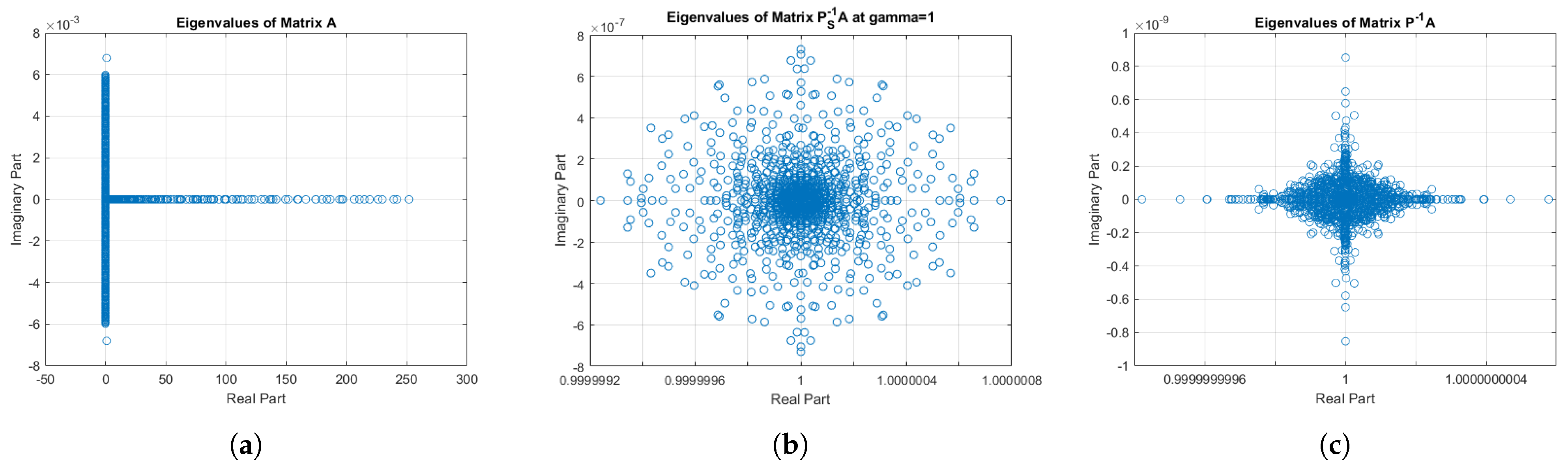
• Our computational analysis indicates that the optimal range for the eigenvalues is concentrated around 1. The most favorable spectrum of eigenvalues is depicted in Figure 4, which illustrates the distribution of eigenvalues across different scenarios. Clearly, our proposed preconditioner $\mathcal{P}$ has a much better spectrum compared to the preconditioner $P_S$ [25] for the Goldhill image of size $512\times 512$.
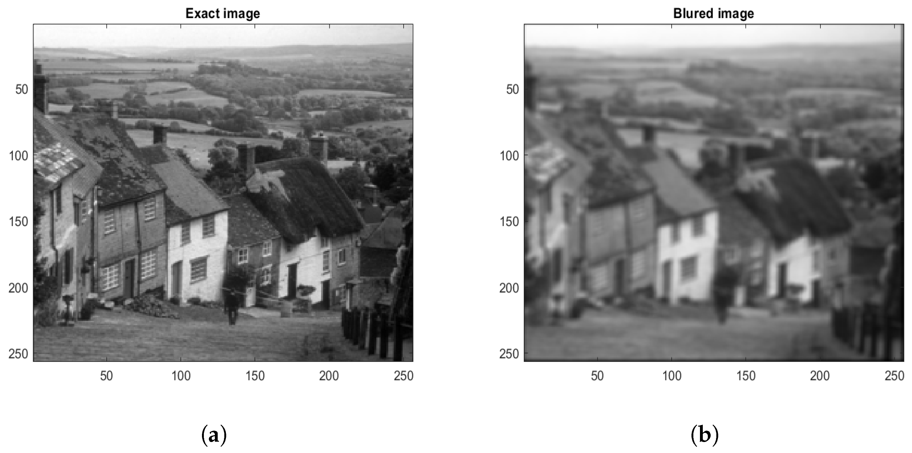
• The effect of preconditioning is clearly demonstrated in Figure 5. It is evident that the $RPBiCGSTAB$ method attained the desired accuracy with substantially fewer iterations than other methods. In contrast, the method without preconditioning (GMRES and BICGSTAB) required over 50 iterations to reach convergence for the Goldhill image of size $512\times 512$. Similar findings were observed for other image dimensions as well.
• All the

  Table 1. The numerical results for Goldhill image.

  ${\mathit{n}}_{\mathit{x}}$	Blurry PSNR	Method	Deblurred PSNR	Error	Iterations	CPU Time
  128	24.7144	GMRES	48.0376	$2.78522\times {10}^{-4}$	46	71.4365
  		BiCGSTAB	48.4597	$2.34269\times {10}^{-8}$	22	21.7596
  		$P_S\mathrm{GMRES}$	49.7696	$9.95176\times {10}^{-8}$	1(2)	18.1246
  		RPBiCGSTAB	49.8697	$2.31212\times {10}^{-12}$	3	16.1349
  256	24.5531	GMRES	47.9646	$2.78522\times {10}^{-4}$	56	91.2974
  		BiCGSTAB	47.4377	$2.83523\times {10}^{-8}$	28	27.7834
  		$P_S\mathrm{GMRES}$	48.7696	$8.91346\times {10}^{-8}$	1(3)	26.3425
  		RPBiCGSTAB	48.9845	$2.78521\times {10}^{-12}$	4	19.3124
  512	24.6983	GMRES	44.2732	$2.78522\times {10}^{-4}$	83	106.7548
  		BiCGSTAB	44.5315	$2.96524\times {10}^{-8}$	37	41.2586
  		$P_S\mathrm{GMRES}$	46.7696	$6.78523\times {10}^{-8}$	2(5)	27.2659
  		RPBiCGSTAB	46.9897	$2.78522\times {10}^{-12}$	6	22.2791

  ,

  Table 2. The numerical results for Moon image.

  ${\mathit{n}}_{\mathit{x}}$	Blurry PSNR	Method	Deblurred PSNR	Error	Iterations	CPU Time
  128	28.4896	GMRES	49.4596	$2.43256\times {10}^{-4}$	48	81.5213
  		BiCGSTAB	49.4789	$2.12896\times {10}^{-8}$	24	31.8512
  		$P_S\mathrm{GMRES}$	50.4578	$8.45896\times {10}^{-8}$	1(3)	19.5963
  		RPBiCGSTAB	50.4586	$2.25693\times {10}^{-12}$	3	16.1349
  256	28.4596	GMRES	48.4786	$2.18963\times {10}^{-4}$	58	95.4963
  		BiCGSTAB	48.3125	$2.12364\times {10}^{-8}$	29	29.1259
  		$P_S\mathrm{GMRES}$	49.4369	$7.14369\times {10}^{-8}$	1(4)	28.1256
  		RPBiCGSTAB	49.1425	$2.13689\times {10}^{-12}$	5	19.1456
  512	28.5429	GMRES	45.4963	$2.74269\times {10}^{-4}$	85	109.8549
  		BiCGSTAB	45.4236	$2.45236\times {10}^{-8}$	41	45.2369
  		$P_S\mathrm{GMRES}$	47.1236	$5.12496\times {10}^{-8}$	2(6)	29.5896
  		RPBiCGSTAB	47.1456	$2.49631\times {10}^{-12}$	7	21.1263

  and

  Table 3. The numerical results for Kids image.

  ${\mathit{n}}_{\mathit{x}}$	Blurry PSNR	Method	Deblurred PSNR	Error	Iterations	CPU Time
  128	23.2189	GMRES	47.1253	$2.25893\times {10}^{-4}$	45	81.1258
  		BiCGSTAB	47.8963	$2.14785\times {10}^{-8}$	22	31.1149
  		$P_S\mathrm{GMRES}$	48.2589	$9.12356\times {10}^{-8}$	1(2)	18.1858
  		RPBiCGSTAB	48.1589	$2.18964\times {10}^{-12}$	3	16.0012
  256	23.1256	GMRES	46.1256	$2.14239\times {10}^{-4}$	55	91.0025
  		BiCGSTAB	46.4589	$2.12569\times {10}^{-8}$	28	27.7034
  		$P_S\mathrm{GMRES}$	47.7589	$8.25814\times {10}^{-8}$	1(3)	26.0421
  		RPBiCGSTAB	47.1526	$2.21852\times {10}^{-12}$	6	17.0125
  512	23.1079	GMRES	43.5896	$2.12846\times {10}^{-4}$	82	106.2109
  		BiCGSTAB	43.8596	$2.85219\times {10}^{-8}$	37	41.2586
  		$P_S\mathrm{GMRES}$	45.5896	$6.14763\times {10}^{-8}$	2(7)	27.2307
  		RPBiCGSTAB	45.1478	$2.14256\times {10}^{-12}$	8	20.4839

  demonstrate that the PSNR achieved by the $RPBiCGSTAB$ method surpasses that of all other methods, including $P_S\mathrm{GMRES}$ [25], and this was accomplished with a significantly reduced number of iterations. The implementation of the $RPBiCGSTAB$ method resulted in a decrease of over $60\%$ in CPU time. Consequently, the $RPBiCGSTAB$ method demonstrated superior performance compared to other methods.
• Figure 1, Figure 2 and Figure 3 clearly illustrate that the $RPBiCGSTAB$ method yielded a slight enhancement in image quality.

7. Conclusions

This study presents an innovative block preconditioning approach tailored for the $5\times 5$ block matrix system arising from the discretization of the Euler–Lagrange equations. The preconditioner is designed to enhance computational efficiency and stability, effectively addressing the complex structures of these discretized equations. We assessed the efficacy of the newly introduced restrictively preconditioned biconjugate gradient-stabilized (RPBiCGSTAB) method in curvature-based image deblurring applications, comparing its performance against established techniques such as GMRES, BiCGSTAB, and $P_S\mathrm{GMRES}$ [25]. This evaluation highlights the RPBiCGSTAB method’s advancements in tackling image deblurring challenges.

Our comprehensive theoretical analysis confirms that this iterative method ensures unconditional convergence with an appropriate matrix splitting strategy, underscoring its robustness across various applications. We also conducted a spectral analysis of the preconditioned matrix, providing critical insights into its eigenvalues and properties, thereby validating our preconditioning strategy.

The performance of the RPBiCGSTAB method was demonstrated through numerical experiments, showcasing its capabilities in image deblurring tasks. Our findings reveal that the RPBiCGSTAB method significantly enhanced the quality of reconstructed images, as indicated by the PSNR metrics. Furthermore, it exhibited a slight improvement in convergence speed compared to GMRES, BiCGSTAB, and $P_S\mathrm{GMRES}$ [25]. This method is efficient, requiring minimal CPU time and achieving rapid convergence within a few iterations, while the eigenvalues of the preconditioned matrix cluster around the value of 1, reinforcing the method’s stability and robustness in practical applications. Beyond image processing, the RPBiCGSTAB can be extended to various other applications, including medical image processing, satellite image analysis, and remote sensing, where similar block-structured systems are prevalent.

References

1. Ren, W.; Deng, S.; Zhang, K.; Song, F.; Cao, X.; Yang, M.-H. Fast ultra high-definition video deblurring via multi-scale separable network. Int. J. Comput. Vis. 2024, 132, 1817–1834. [Google Scholar] [CrossRef]
2. Ren, W.; Wu, L.; Yan, Y.; Xu, S.; Huang, F.; Cao, X. INformer: Inertial-Based Fusion Transformer for Camera Shake Deblurring. IEEE Trans. Image Process. 2024, 33, 6045–6056. [Google Scholar] [CrossRef]
3. Chen, K. Introduction to variational image-processing models and applications. Int. J. Comput. Math. 2013, 90, 1–8. [Google Scholar] [CrossRef]
4. Sun, L.; Chen, K. A new iterative algorithm for mean curvature-based variational image denoising. BIT Numer. Math. 2014, 54, 523–553. [Google Scholar] [CrossRef]
5. Yang, F.; Chen, K.; Yu, B.; Fang, D. A relaxed fixed point method for a mean curvature-based denoising model. Optim. Methods Softw. 2014, 29, 274–285. [Google Scholar] [CrossRef]
6. Zhu, W.; Chan, T. Image denoising using mean curvature of image surface. SIAM J. Imaging Sci. 2012, 5, 1–32. [Google Scholar] [CrossRef]
7. Zhu, W.; Tai, X.C.; Chan, T. Augmented Lagrangian method for a mean curvature based image denoising model. Inverse Probl. Imaging 2013, 7, 1409–1432. [Google Scholar] [CrossRef]
8. Fairag, F.; Chen, K.; Ahmad, S. An effective algorithm for mean curvature-based image deblurring problem. Comput. Appl. Math. 2022, 41, 176. [Google Scholar] [CrossRef]
9. Fairag, F.; Chen, K.; Ahmad, S. Analysis of the CCFD method for MC-based image denoising problems. Electron. Trans. Numer. Anal. 2021, 54, 108–127. [Google Scholar] [CrossRef]
10. Mobeen, A.; Ahmad, S.; Fairag, F. Non-blind constraint image deblurring problem with mean curvature functional. Numer. Algorithms 2025, 98, 1703–1723. [Google Scholar] [CrossRef]
11. Khalid, R.; Ahmad, S.; Medani, M.; Said, Y.; Ali, I. Efficient preconditioning strategies for accelerating GMRES in block-structured nonlinear systems for image deblurring. PLoS ONE 2025, 20, e0322146. [Google Scholar] [CrossRef]
12. Fairag, F.; Chen, K.; Brito-Loeza, C.; Ahmad, S. A two-level method for image denoising and image deblurring models using mean curvature regularization. Int. J. Comput. Math. 2022, 99, 693–713. [Google Scholar] [CrossRef]
13. Ahmad, S.; Fairag, F. Circulant preconditioners for mean curvature-based image deblurring problem. J. Algorithms Comput. Technol. 2021, 15, 17483026211055679. [Google Scholar] [CrossRef]
14. Ahmad, S.; Al-Mahdi, A.M.; Ahmed, R. Two new preconditioners for mean curvature-based image deblurring problem. AIMS Math. 2021, 6, 13824–13844. [Google Scholar] [CrossRef]
15. Beik, F.P.A.; Benzi, M. Preconditioning techniques for the coupled Stokes–Darcy problem: Spectral and field-of-values analysis. Numer. Math. 2022, 150, 257–298. [Google Scholar] [CrossRef]
16. Kim, J.; Ahmad, S. On the preconditioning of the primal form of TFOV-based image deblurring model. Sci. Rep. 2023, 13, 17422. [Google Scholar] [CrossRef]
17. Saad, Y. A flexible inner-outer preconditioned GMRES algorithm. SIAM J. Sci. Comput. 1993, 14, 461–469. [Google Scholar] [CrossRef]
18. Cao, Y.; Jiang, M.Q.; Zheng, Y.L. A splitting preconditioner for saddle point problems. Numer. Linear Algebra Appl. 2011, 18, 875–895. [Google Scholar] [CrossRef]
19. Knight, F.M.; Wathen, A.J.; Trefethen, L.N. The BiCGSTAB method for solving large sparse linear systems. SIAM J. Sci. Stat. Comput. 1994, 15, 237–248. [Google Scholar]
20. Saad, Y. Iterative Methods for Sparse Linear Systems, 2nd ed.; Society for Industrial and Applied Mathematics (SIAM): Philadelphia, PA, USA, 2003; pp. 1–462. [Google Scholar]
21. Van der Vorst, H.A. BiCGSTAB: A fast and robust iterative solver for large, sparse, non-symmetric linear systems. Numer. Linear Algebra Appl. 2003, 10, 79–94. [Google Scholar]
22. Chen, J.; Li, Y.; Zhang, Z. Efficient implementation of BiCGSTAB for large-scale sparse linear systems with preconditioning. J. Comput. Appl. Math. 2018, 334, 343–356. [Google Scholar]
23. Bouyghf, A.; Abdessalem, M. An enhanced version of the BiCGSTAB method with global and block orthogonal projectors. Numer. Linear Algebra Appl. 2023, 30, 201–221. [Google Scholar]
24. Tadano, Y.; Kuramoto, H. A block-wise updating method for BiCGSTAB with applications to multiple right-hand sides. J. Appl. Comput. Math. 2019, 6, 100–120. [Google Scholar]
25. Ahmad, S. Optimized five-by-five block preconditioning for efficient GMRES convergence in curvature-based image deblurring. Comput. Math. Appl. 2024, 175, 174–183. [Google Scholar] [CrossRef]
26. Lysaker, M.; Osher, S.; Tai, X.C. Noise removal using smoothed normals and surface fitting. IEEE Trans. Image Process. 2004, 13, 345–1457. [Google Scholar] [CrossRef]
27. Brito, C.; Chen, K. Multigrid algorithm for high order denoising. SIAM J. Imaging Sci. 2010, 3, 363–389. [Google Scholar] [CrossRef]
28. Rui, H.; Pan, H. A block-centered finite difference method for the DarcyForchheimer model. SIAM J. Numer. Anal. 2012, 5, 2612–2631. [Google Scholar] [CrossRef]
29. Vogel, C.R.; Oman, M.E. Fast, robust total variation-based reconstruction of noisy, blurred images. IEEE Trans. Image Process. 1998, 7, 813–824. [Google Scholar] [CrossRef]
Figure 1. Goldhill image: (a) shows the original image; (b) presents the blurred version; (c) displays the deblurred result using GMRES; (d) shows the deblurred image obtained via BiCGSTAB; (e) depicts the deblurred image produced by P S GMRES ; (f) illustrates the deblurred image using RPBiCGSTAB.
Mca 30 00076 g001aMca 30 00076 g001b
Figure 2. Moon image: (a) presents the original image; (b) displays the blurred image; (c) shows the deblurred result obtained with GMRES; (d) illustrates the deblurred image produced using BiCGSTAB; (e) depicts the deblurred image from P S GMRES ; (f) demonstrates the deblurred image achieved with RPBiCGSTAB.
Mca 30 00076 g002aMca 30 00076 g002b
Figure 3. Kids image [8]: (a) presents the original image; (b) shows the blurred image; (c) depicts the deblurred image obtained with GMRES; (d) illustrates the deblurred image produced by BiCGSTAB; (e) displays the deblurred image generated using P S GMRES ; (f) demonstrates the deblurred image achieved with RPBiCGSTAB.
Mca 30 00076 g003aMca 30 00076 g003b
Figure 4. The eigenvalue distributions of matrices (a) A , (b) P S 1 A , and (c) P 1 A for Goldhill image of size 512 × 512 .
Mca 30 00076 g004
Figure 5. Residual norms and first 50 iteration counts for GMRES, BiCGSTAB, RPBiCGSTAB, and P S GMRES for Goldhill image of size 512 × 512 .
Mca 30 00076 g005