Simulation of Temperature Field in Steel Billets during Reheating in Pusher-Type Furnace by Meshless Method

Abstract

Using a meshless method, a simulation of steel billets in a pusher-type reheating furnace is carried out for the first time. The simulation represents an affordable way to replace the measurements. The heat transfer from the billets with convection and radiation is considered. Inside each of the billets, the heat diffusion equation is solved on a two-dimensional central slice of the billet. The diffusion equation is solved in a strong form by the Local Radial Basis Function Collocation Method (LRBFCM) with explicit time-stepping. The ray tracing procedure solves the radiation, where the view factors are computed with the Monte Carlo method. The changing number of billets in the furnace at the start and the end of the loading and unloading of the furnace is considered. A sensitivity study on billets’ temperature evolution is performed as a function of a different number of rays used in the Monte Carlo method, different stopping times of the billets in the furnace, and different spacing between the billets. The temperature field simulation is also essential for automatically optimizing the furnace’s productivity, energy consumption, and the billet’s quality. For the first time, the LRBFCM is successfully demonstrated for solving such a complex industrial problem.

1. Introduction

Reheating steel billets after continuous casting is necessary to temper the billets for hot rolling. Steel billets are usually heated up to 1200 °C. Five types of continuous industrial reheating furnaces are known for moving steel billets inside the furnace [1], of which the walking beam and pusher industrial reheating furnaces are the most widely used types in the steel industry. This work is focused on the simulation of temperature conditions in the gas-fired pusher-type furnace [2]. These furnaces operate mostly in a continuous mode. The steel billets are charged at the furnace entry, heated while stepwise moving inside the furnace, and released at the furnace exit [3]. The continuous mode of this process is interrupted at the start of charging until the furnace is filled up and at the end of the process, when the billets are only discharged without charging.

Heat is transferred to each steel billet by moving inside the furnace from the furnace entry to the furnace exit. The heat transfer mechanisms include radiation from the gases of the burners, radiation from the furnace walls, and convection [4]. The heat transfer by thermal radiation accounts for more than 90% of the total heat flux impinging on the billet surface [5]. The required temperature of the billets at the furnace outlet is determined by the hot rolling requirements, which consider the size of the billets, rolling speed, and steel composition [6,7]. The process should ensure the required uniform temperature distribution of the billet at discharge from the furnace.

The control of the furnace, natural gas consumption, and productivity mainly depend on the knowledge of the temperature field of the billets. Measuring the temperature inside the billets with thermocouples is possible for experimental purposes only. However, performing such measurements in a standard way during production is impossible. Computer simulation thus represents an affordable way to replace the mentioned measurements. The temperature field simulation is also essential for automatically optimizing the furnace’s productivity, energy consumption, and the billet’s quality. Automatic optimization is performed by calculating the related object functions and using the evolutionary optimization algorithm to minimize them. Several simulation models have already been developed to predict the reheating process of steel billets in a reheating furnace. The first published model on the heating process in regenerative furnaces considering the moving billets was introduced in [8]. A simplified furnace geometry was considered, and the billets were modeled as a single body located on the furnace floor. Later, Kim and Huh [9] modeled the thermal behavior of the furnace system as a steady-state heating process. The temperature field of the billets has been calculated using the finite difference technique. Hsieh et al. [10] applied the model introduced in [9] to model the turbulent flow of the combustion process using complex real-world furnace geometry. The details are provided in [1].

The solution of the temperature field in the middle of each of the billets during the reheating process is, in the present work, obtained based on the meshless Local Radial Basis Function Collocation Method (LRBFCM) with explicit time-stepping for the first time. This method has already been demonstrated for solving different steel processing steps such as continuous casting [11], hot rolling [12], cooling at the cooling bed after rolling [13], and microstructure evolution [14].

2. Thermal Model

2.1. Heat Transfer Equation

The temperature field in the steel billets is governed by the heat diffusion equation

$$\frac{\partial }{\partial t}\left(\rho h\right)=\nabla \cdot \left(k\nabla T\right),$$

(1)

where $\rho , h, T$, and $k$ stand for density, mass-specific enthalpy, temperature, and thermal conductivity, respectively. It is assumed that the relation

$$h\left(T\right)=c_p\left(T\right)T,$$

(2)

with $c_p\left(T\right)$ standing for the, in general, temperature-dependent specific heat at constant pressure.

2.2. Boundary Conditions

Neumann boundary condition is employed as a magnitude of heat flux $q$ in the normal direction $n$ on the boundary

$$q_n=q\cdot n=-k\frac{\partial T}{\partial n}=c_{conv}{q}_{conv}+q_{radS}+c_{BG}{q}_{radBG}+c_G{q}_{radG},$$

(3)

where the heat flux inside the billet is defined by Fourier’s law $q=-k\nabla T$. The total heat flux is composed of the convective heat flux $q_{conv}$, radiative heat flux from the surface of the furnace and billets inside the furnace $q_{radS}$, radiative heat flux from the burning gas $q_{radBG}$, and radiative heat flux from the inner gas $q_{radG}$. The constants $c_{conv}, c_{BG}, c_G$ depend on the shape, position of the billets, and the position of the furnace’s inner walls.

The billets are positioned close to the bottom of the furnace. So, the bottom of the billets only receives the radiation from the bottom of the furnace. The burning gas influences from the top of the furnace. The top of the billets receives radiation from all the contributors. The radiation from the burning gas to the billet is geometrically shadowed by the neighboring billets situated at the left or right side of the considered billet. The constants $c_{conv}, c_{BG}, c_G$ for the surface of billets are shown in Table 1, where $d$ is the distance between two neighboring billets; $w_b$ is the square dimension of the billets. Since there is no obstruction from other billets, the constants are $c_{conv}=1, c_{BG}=1/2, c_G=1$ on the left side of the first billet, the right side of the last billet, and the edge of all billets, respectively.

Table 1. Coefficients of heat flux for different surfaces of billets.

	Top	Left–Right	Bottom
$c_{conv}$	1	1	0
$c_{BG}$	1	$\left[\arctan (d/W_B)\right]/\pi$	0
$c_G$	1	1	0

2.2.1. Radiative Heat Flux

The furnace has dimensions $L_F\times W_F\times H_F$ (length, width, and height). A symmetry plane is considered at $W_F/2$. The billets have dimensions $L_B\times W_B\times H_B$, and there is a space between the billets, denoted by $S_B$. The distance between the bottom of the billets and furnace bottom is denoted by $D_{FB}$. The distance of the center of the first billet from the start surface of the furnace is $D_{LBe}$, and the center position of the last billet from the end surface of the furnace is denoted by $D_{LBo}$. The billets are moving from the start to the end surface of the furnace.

The radiative heat flux from the surface of the furnace and billets is calculated in three dimensions and used to calculate the temperature in the two-dimensional middle slices of each of the billets. The surface of the furnace and the billets is divided into finite surface planes (FSPs), depicted in Figure 1.

Figure 1. A scheme of the division of the involved surfaces into FFSs. (a) A scheme of the furnace planes, and (b) a scheme of the billet planes.

The furnace length $L_F$ is divided into $N_L$ equidistant segments with top, bottom, front, and back surfaces. The furnace’s start and the end surfaces are divided into $N_H$ vertically positioned equidistant surfaces. The billets are in the longitudinal direction divided into three segments, of which only one and a half of the central segment is considered due to the symmetry. The top, bottom, left, and right surfaces of each of the three segments are divided into two equidistant surfaces (2 × 8 in total). The temperatures of the billets are calculated in the middle of the second longitudinal segment. Each billet’s head and tail are divided into four equal surfaces.

The net radiative heat flux of the i-th FSP $q_{\mathit{radS},i}$ is given as a difference between the emitted heat flux from the i-th surface and received heat flux from all surrounding FSPs written as

$$q_{\mathit{radS},i}={\displaystyle \sum _{j=1}^J{\epsilon }_j(T_j)\sigma T_j^4\frac{A_j}{A_i}{F}_{j\to i}}-{\alpha }_i(T_i)\sigma T_i^4,$$

(4)

where $T_j$ is the average temperature of the j-th FSP, and the sum goes over all $J$ FSPs, where $A_j$ represents the area of the j-th FSP. The visibility between FSPs is given by a view factor F_j→i ∈ [0, 1]. It defines the fraction of the radiation emitted by the j-th FSP and received by the i-th FSP [15]. A ray tracing algorithm is used in the simulations. The number of rays is defined per square meter of the surfaces involved. The rays are randomly emitted and tracked until they are absorbed.

The temperatures $T_{Bs}, s=1,2,3,4$ of the four head and four tail planes of each of the billets are calculated by solving Equation (1) four times in one dimension by assuming the Dirichlet boundary condition at the center of each quarter of the middle slice from the 2D calculation and the Neumann boundary condition in Equation (2) of each plane at the head of the billet (Figure 2a).

Figure 2. A scheme of the division of the billets to calculate the average temperature for each plane of the billets. (a) A whole billet with 32 planes and middle slice, (b) half of the billet showing two planes i and j from the first segment, (c) half of the billet showing two planes m and n from the second segment, and (d) half of the billet showing the connection between the middle and head planes.

The one-dimensional equations are calculated by the finite difference method

$${\rho }_{0l}{c}_{p0l}\frac{T_l-T_{0l}}{\Delta t}=\frac{k_{0l}-k_{0l-1}}{\Delta z}\frac{T_{0l}-T_{0l-1}}{\Delta z}+\frac{T_{0l+1}-2T_{0l}+T_{0l-1}}{\Delta z^2},$$

(5)

where subscripts 0 and l indicate the initial time-step and the position of the point. Half of the billet length is represented by 201 equidistant nodes. $T_{\mathrm{Cs}}=T_1$ is the average temperature value of a quarter of the middle slice (Figure 2d) computational domain of the billet. $T_{Bs}=T_{201}$ (in Figure 2d) is used as the average temperature of the head plane of the billet in Equation (6). The temperature $T_m$ of plane m (in Figure 2c) is the average temperature value of the boundary nodes belonging both to the 2D slice and plane m. The temperature $T_n$ of plane n is calculated in the same way as the temperature of plane m. The temperature of the planes i and $j$ (in Figure 2b) is $T_i=(T_{\mathrm{B}1}+T_m)/2$ and $T_j=(T_{\mathrm{B}1}+T_n)/2$. This procedure is repeated four times in order to cover all four sides of the billet. The temperature of the billets is the same at the head as at the tail because of the symmetry.

The radiative heat flux from the burning gas $q_{radBG}$ and the radiative heat flux from the inner gas $q_{radG}$ are described as the difference between the emitted heat flux from the gas and the heat flux emitted from the billets

$$q_{radBG}={\alpha }_{BG}\sigma (T_{BG},T)T^4-{\epsilon }_{BG}(T_{BG})\sigma T_{BG}^4,$$

(6)

$$q_{radG}={\alpha }_G\sigma (T_G,T)T^4-{\epsilon }_G(T_G)\sigma T_G^4,$$

(7)

where $\sigma =5.6704\times {10}^{-8}{ \mathrm{Wm}}^{-2}{\mathrm{K}}^{-4}$ is the Stefan–Boltzmann constant, $\alpha$ is the absorption of the gas, $\epsilon$ is the emissivity of the gas [16], and $T_{BG}$ and $T_G$ stand for the temperature of the burning gas and inner gas, respectively. $T_{BG}$ is obtained from the balance of the heat flux at the central point of the front furnace wall when the furnace is empty. The temperature of the inner gas is considered the same as the temperature of the nearest furnace wall (see [17]).

2.2.2. Convective Heat Flux

The convective heat flux $q_{conv}$ is specified as

$$q_{conv}=h(T-T_{Gas}),$$

(8)

where $h$ and $T_{Gas}$ stand for the heat transfer coefficient and inner gas temperature, respectively.

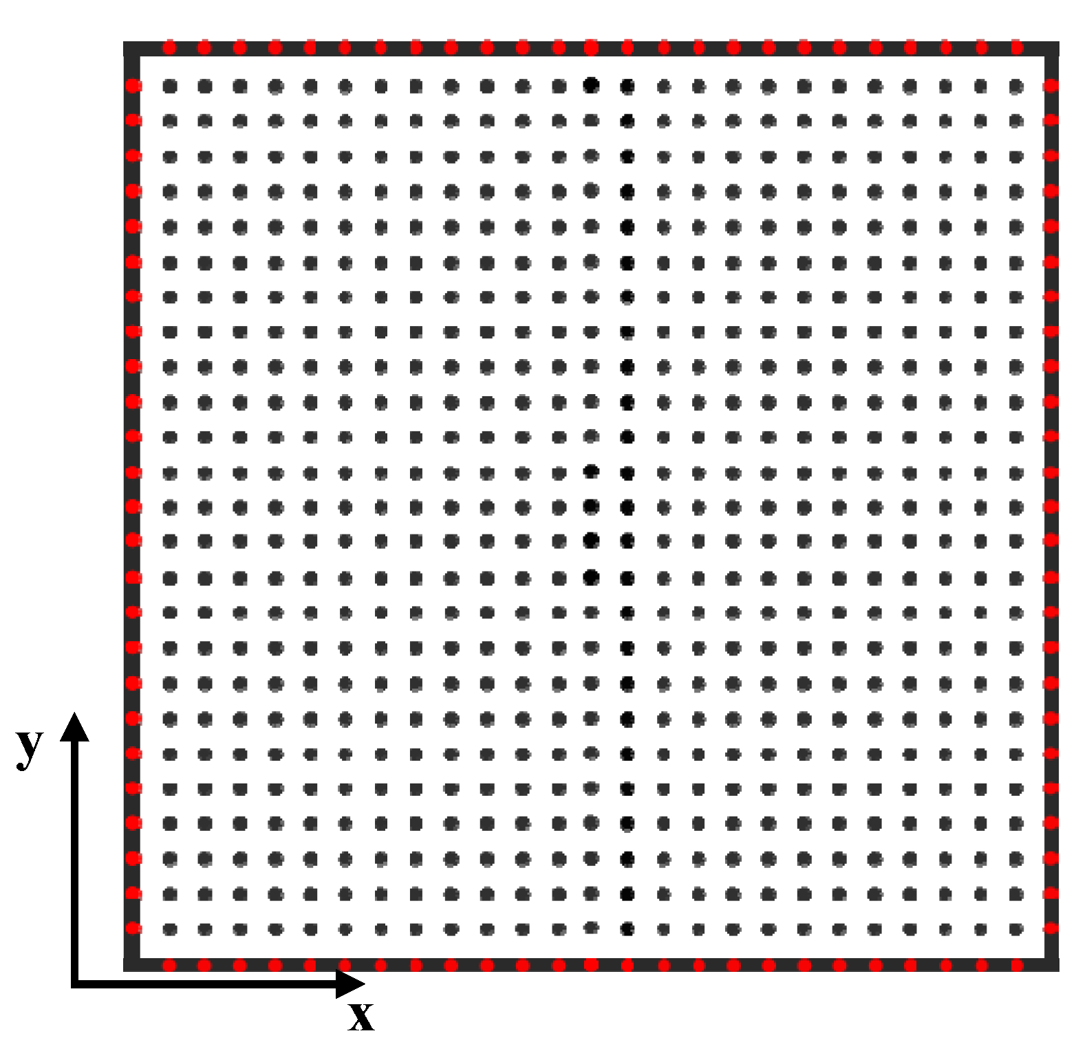
3. Solution Procedure

The temperature field is solved by the LRBFCM [18] on a 2D slice, representing the billet cross-section, described in the Cartesian coordinate system. Instead of a grid generation over the computational domain, such as in FEM, collocation nodes without any special geometrical connectivity are uniformly distributed over the domain and at the boundaries. An unknown scalar or vector component field $\theta \left(p\right)$ at position $p=p_x{i}_x+p_y{i}_y$ ($p_x,p_y$ are Cartesian components and $i_x,i_y$ are orthonormal Cartesian base vectors) is interpolated with multi-quadric RBF $\psi \left(p\right)$ together with the augmented first-order $\left(N_p=3\right)$ polynomials $\vartheta \left(p\right)$ over the neighboring $\left(N=7\right)$ nodes (see Figure 3)

$${\psi }_i\left(p\right)=\sqrt{{\left(c\frac{p_x-p_{xi}}{x_{\max }}\right)}^2+{\left(c\frac{p_y-p_{yi}}{y_{\max }}\right)}^2+1}; i=1,2,\dots ,N,$$

$${\vartheta }_{N+1}\left(p\right)=1, {\vartheta }_{N+2}\left(p\right)=p_x-p_{x0}, {\vartheta }_{N+3}\left(p\right)=p_y-p_{y0}.$$

Figure 3. Meshless domain and boundary discretization scheme with local influence domains consisting of 7 nodes. Influence domains with boundary nodes (red doted lines) and with only internal nodes (black dotted lines) are shown.

$x_{\max }$ and $y_{\max }$ are the maximum horizontal and vertical distances between the considered nodes. $p_{x0},p_{y0}$ are the coordinates of the central node inside the influence domain, and c is the multi-quadric shape parameter. The collocation thus reads

$$\theta \left(p\right)={\displaystyle \sum _{i=1}^N{\psi }_i\left(p\right){\alpha }_i}+{\displaystyle \sum _{i=1}^{N_p}{\vartheta }_i\left(p\right){\alpha }_{N+i}}.$$

(9)

The first and second partial derivatives are obtained from the interpolation as follows

$$\frac{\partial \theta \left(p\right)}{\partial p_{x_j}}={\displaystyle \sum _{i=1}^N\frac{\partial {\psi }_i\left(p\right)}{\partial p_{x_j}}{\alpha }_i}+{\displaystyle \sum _{i=1}^{N_p}\frac{\partial {\vartheta }_i\left(p\right)}{\partial p_{x_j}}{\alpha }_{N+i}}, \frac{{\partial }^2\theta \left(p\right)}{\partial p_{x_j}^2}={\displaystyle \sum _{i=1}^N\frac{{\partial }^2{\psi }_i\left(p\right)}{\partial p_{x_j}^2}{\alpha }_i}+{\displaystyle \sum _{i=1}^{N_p}\frac{{\partial }^2{\vartheta }_i\left(p\right)}{\partial p_{x_j}^2}{\alpha }_{N+i}}.$$

(10)

The explicit solution of the governing equation of the thermal model is considered

$$\rho c_p\frac{T_i-T_{0i}}{\Delta t}=\nabla \cdot \left(k\nabla T_{0i}\right).$$

(11)

The temperature field $T\left(p\right)$ in the thermal model is interpolated in the sense of Equation (9)

$$T\left(p\right)={\displaystyle \sum _{i=1}^N{\psi }_i{\left(p\right)}_T{\alpha }_i}+{\displaystyle \sum _{i=1}^{N_p}{\vartheta }_i{\left(p\right)}_T{\alpha }_{N+i}}.$$

(12)

The details of the solution procedure are provided in [19].

4. Numerical Examples

This section shows the verification of the calculation of view factors (Example 1) and the thermal model (Example 2). Afterwards, the simulation results of an actual reheating furnace are demonstrated with different process parameter configurations. Case 1 is calculated with three different ray densities. Case 2 is calculated with two different stopping times. Case 3 is calculated with different spacing between billets. In all the simulations, emissivity $\epsilon$ and absorption coefficients $\alpha$ are 0.8, and the time-step $\Delta t$ for the explicit solution is 0.1 s. The shape parameter $c={10}^{-3}$ is used in the meshless method (MM). Since the interpolation function is based on the scaled RBF, the results are not sensitive to $c$. A suitable shape parameter is obtained during the comparison with the reference solution and used in our related similar simulations. The details of the choice of $c$ are shown in [19]. Results in Section 4.1 and Section 4.2 are compared with Finite Volume Method (FVM).

4.1. Verification of Calculation of View Factors

The computational model’s accuracy strongly depends on the accuracy of the calculation of view factors. First, it has to be proven that the view factors are correctly calculated, and second, as the number of rays increases, the results should converge to the exact solution. For this purpose, we have created a sample test environment, as shown in Figure 4. A steel billet is put inside a very long furnace, and only a small section, 400 mm long, is considered. Both ends of this section are considered to have perfect reflectivity. Just like in the reheating furnace simulations, we have calculated the view factors in 3D. The heat flux results are calculated at the middle thickness.

Figure 4. A section of the furnace with a steel billet in the middle, 400 mm long.

To verify the view factors, we focused on calculating the radiative heat flux on the boundaries of the billet. We compared our heat flux results with the results obtained by a reference solution computed with [20]. In this case, the only source of heat flux at the boundaries is due to radiation from the other surfaces. Each furnace wall is divided into 160 planes, and each of the billet’s sides are divided into 18 planes. Each of these planes has a dimension of 10 mm × 400 mm (width × length). There is no need for division along the 400 mm length of the furnace since the results do not change on that axis. Since the wall temperatures of the furnace and billet are fixed, the only error would come from the calculation process of the view factors. The results are shown in Figure 5. The computational domain is considered to be in the middle cross-section of the billet with a size of 180 mm × 180 mm. Uniform node distribution with 25 nodes at each side of the billet is used, and three different ray densities (${10}^6/{\mathrm{m}}^2, {10}^7/{\mathrm{m}}^2, {10}^8/{\mathrm{m}}^2$) are randomly sent from each square meter. It is evident from Figure 5 that the view factors are correctly calculated, and with the increase in the number of the rays, the results converge to the reference value. The reference solution is also obtained by the ray tracing algorithm, and both simulations use the same number of planes.

Figure 5. Heat flux on boundary with different rays emitted from each plane with Monte Carlo method at $t=0$ s.

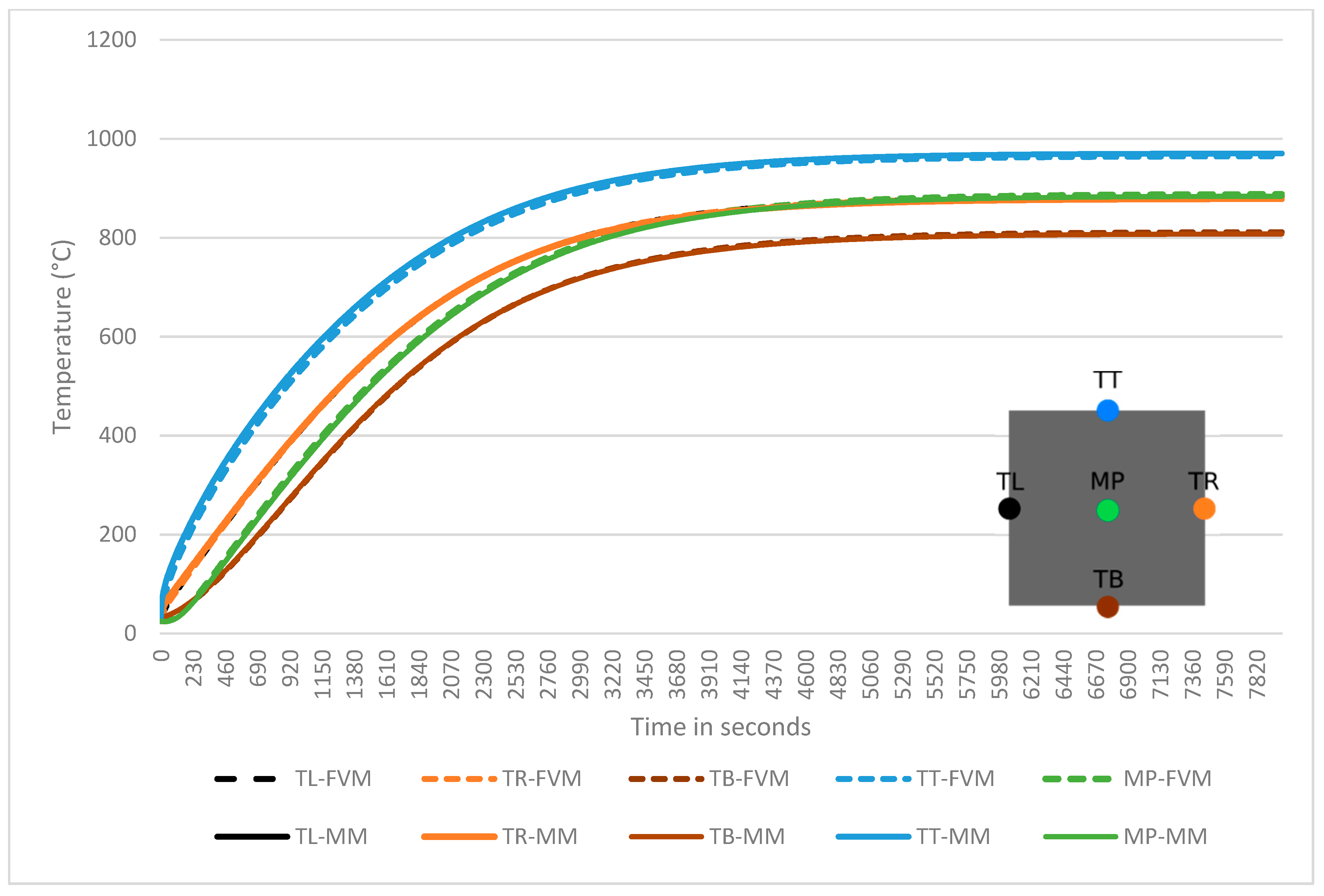
4.2. The Verification of the Simulation Model of the Reheating Furnace

Once the calculation of the view factors is verified, the results in terms of temperature should also be verified. This time, the steel billet is positioned just above the bottom, like in a real furnace. This is a time-dependent process, and simulations are run up to 8000 s. in both simulations based on five reference points that are chosen in the billet, as shown in Figure 6. Both the MM and FVM temperature results for those five points are shown in Figure 7 as a function of time. In Figure 8, the temperature fields of the steel billet at 8000 s are shown. As expected, good agreements have been once again obtained. All the parameters used in the verification processes are listed in Table 2.

Figure 6. A small cross-section of the furnace with a steel billet on the bottom, 400 mm long.

Figure 7. A comparison of the results from the simulation and reference solution.

Figure 8. The temperature field of the steel billet at 8000 s, computed by (a) the LRBFCM and (b) FVM.

Table 2. Benchmark parameters.

Density ($\rho$)	kg/m3	7500
Specific heat (cp)	J/kg K	600
Thermal conductivity (k)	W/m K	40
Initial temperature (T)	°C	25
Observed time (t_end)	s	8000

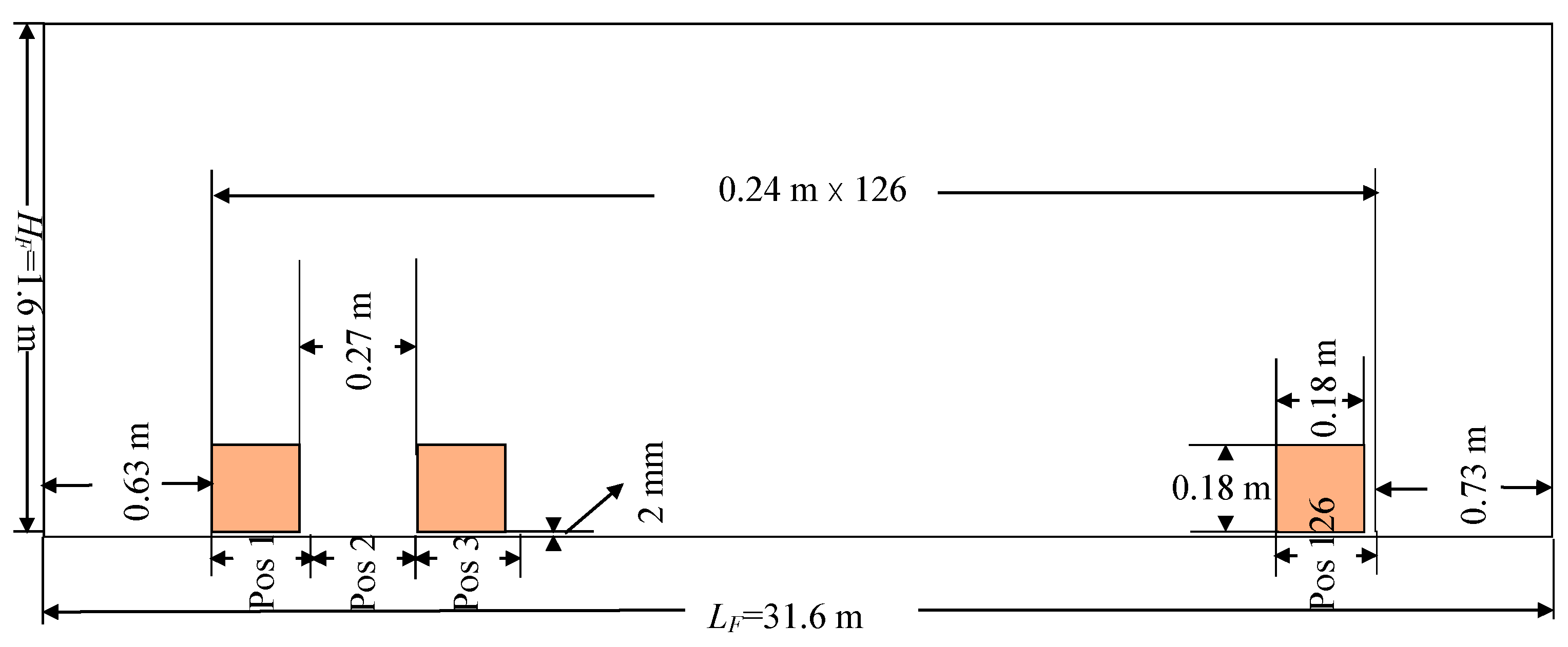
4.3. Sensitivity Studies of an Industrial Reheating Furnace Simulation

We focus on the central cross-section of the billets by assuming no heat transfer along the length direction, since the longitudinal dimensions of the billets are large compared to the transversal dimensions. The billets with a square cross-section of 0.18 m × 0.18 m ($W_B\times H_B$) and length of 4 m ($L_B$) were studied. The internal dimensions of the furnace are $31.6 \mathrm{m} \times 4.8 \mathrm{m} \times 1.6 \mathrm{m}$ ($L_F\times W_F\times H_F$). The distance of the center of the first billet from the start surface of the furnace is $D_{LBe}=0.72 \mathrm{m}$ There are 126 positions (pos in Figure 9) with a width of $0.24 \mathrm{m}$ in the furnace. The distance between the bottom of the billets and furnace bottom is $D_{FB}=0.002 \mathrm{m}$ (see Figure 9). The billets are positioned centrally along the width of the furnace, so only 0.4 m space is left at both ends. In this work, the surface of the furnace is divided into 128 planes ($N_L=30, N_H=4$). The surface of each billet is divided into 32 planes (top, bottom, left, and right: six planes. Head and tail: four planes), as in Figure 1b. The temperature of the surface of the furnace $T_j$ is the same as that used in [17].

Figure 9. The cross-section of the furnace with the billets. One space between neighboring billets. There are 63 billets in the furnace.

All the billets move from the previous position to the next in a stopping time interval $\Delta t$. One new billet is transported in the furnace from the start side, and one is transported out of it from the end side when the furnace is full. Natural gas burners are positioned at the top of the furnace. The billets are made of steel type 70MnVS4. The temperature-dependent material properties are considered as obtained from JmatPro [21]. A total of 725 uniformly distributed points on the middle slice (see Figure 10) of each billet and subdomains with seven nodes are used in the LRBFCM. The room temperature of 25 °C is used as the initial temperature of the billets.

Figure 10. Sketch of the middle slice with uniformly distributed points. Red points are on the boundaries and black points are in the domain.

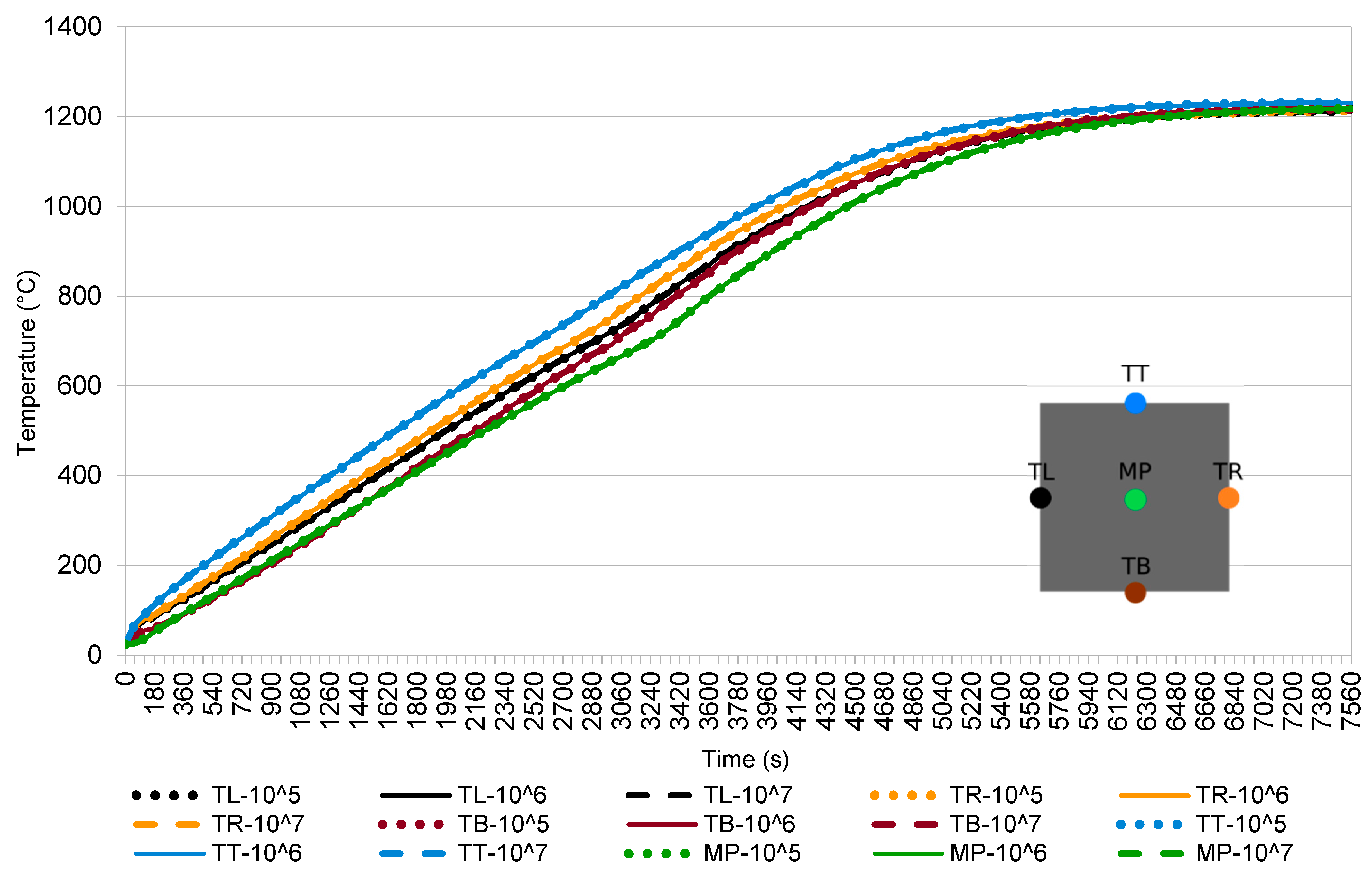
4.3.1. Case 1: Different Number of Rays Used in View Factors

In Case 1, the space between the billets is $S_B=0.27 \mathrm{m}$ between each neighboring two billets. The billets stop at each position for 60 s. ${10}^5/{\mathrm{m}}^2, {10}^6/{\mathrm{m}}^2, {10}^7/{\mathrm{m}}^2$ ray densities are used for the Monte Carlo method to calculate the view factor, respectively. The results are shown in Figure 11.

Figure 11. The results of Case 1: the temperature field in 5 representative points of the billet as a function of different ray densities per m².

In Case 1, three different view factors’ results are used for different positions and compared. The Monte Carlo ray tracing method is probabilistic. Therefore, each time the view factors are calculated, the results fluctuate. The magnitude of fluctuation may be reduced by increasing the number of ray samples. When the results are summed up, parts of the errors (over/under fluctuations) are cancelled out. That is why the difference in the results in this case is so small. Moreover, the result of the Monte Carlo method for calculating the view factors depends on the number of random trials. It takes approximately 2 days to calculate the view factors when 63 billets are in the furnace by using Intel Xeon 6146 CPU.

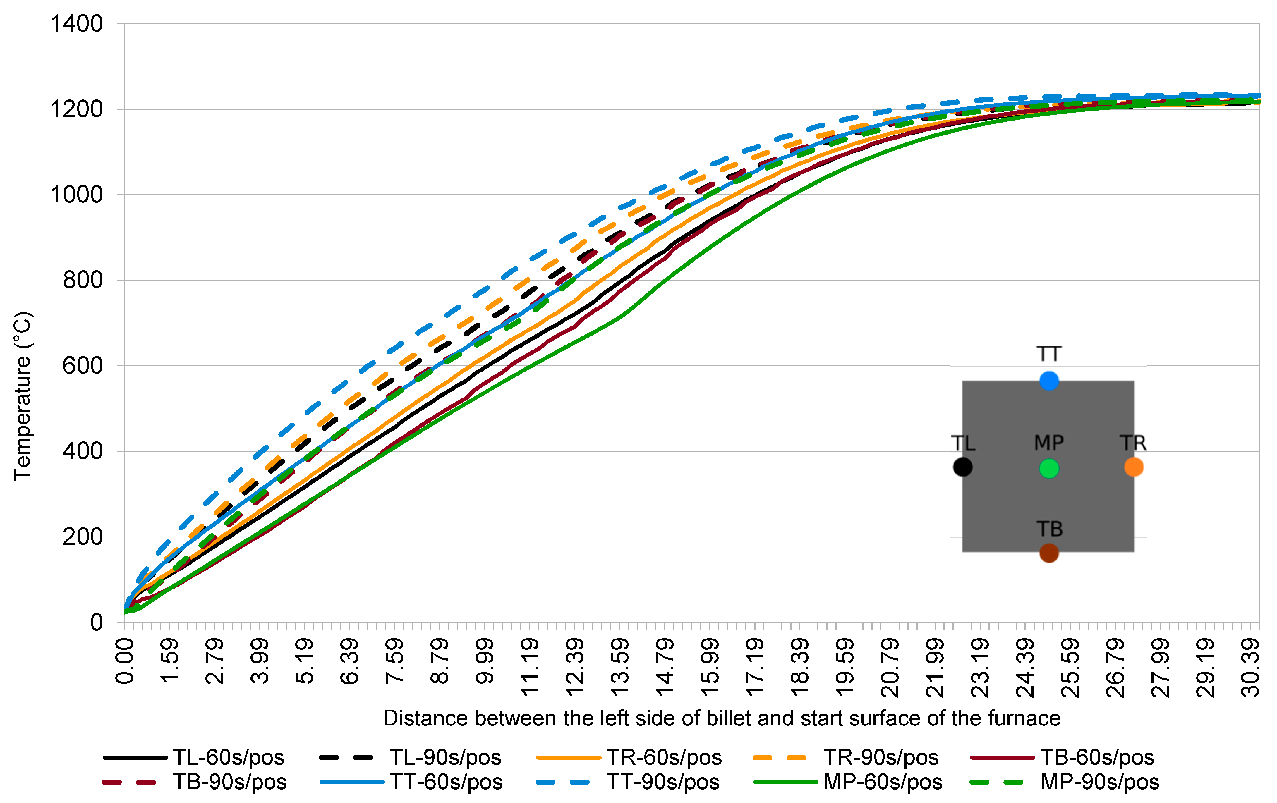
4.3.2. Case 2: Different Stopping Times at Each Position

In Case 2, the space between the billets is $S_B=0.27 \mathrm{m}$ between each neighboring two billets. The cross-section of the furnace with the billets is shown in Figure 9. The billets stop at each position for 60 s and 90 s, respectively. Additionally, ${10}^6/{\mathrm{m}}^2$ ray densities are used in the Monte Carlo method to calculate the view factors. The results are shown in Figure 12.

Figure 12. The results of Case 2: the temperature field in 5 representative points of the billets as a function of different stopping times at each position.

We see that the temperatures for the 90 s stopping time are higher than those with the 60 s stopping time. However, both results reach 1200 °C at the furnace end, and the billet has almost a uniform temperature. We observe a slightly different behavior of the billet center at temperatures between 700 °C and 800 °C because of the changes in the material properties due to phase change.

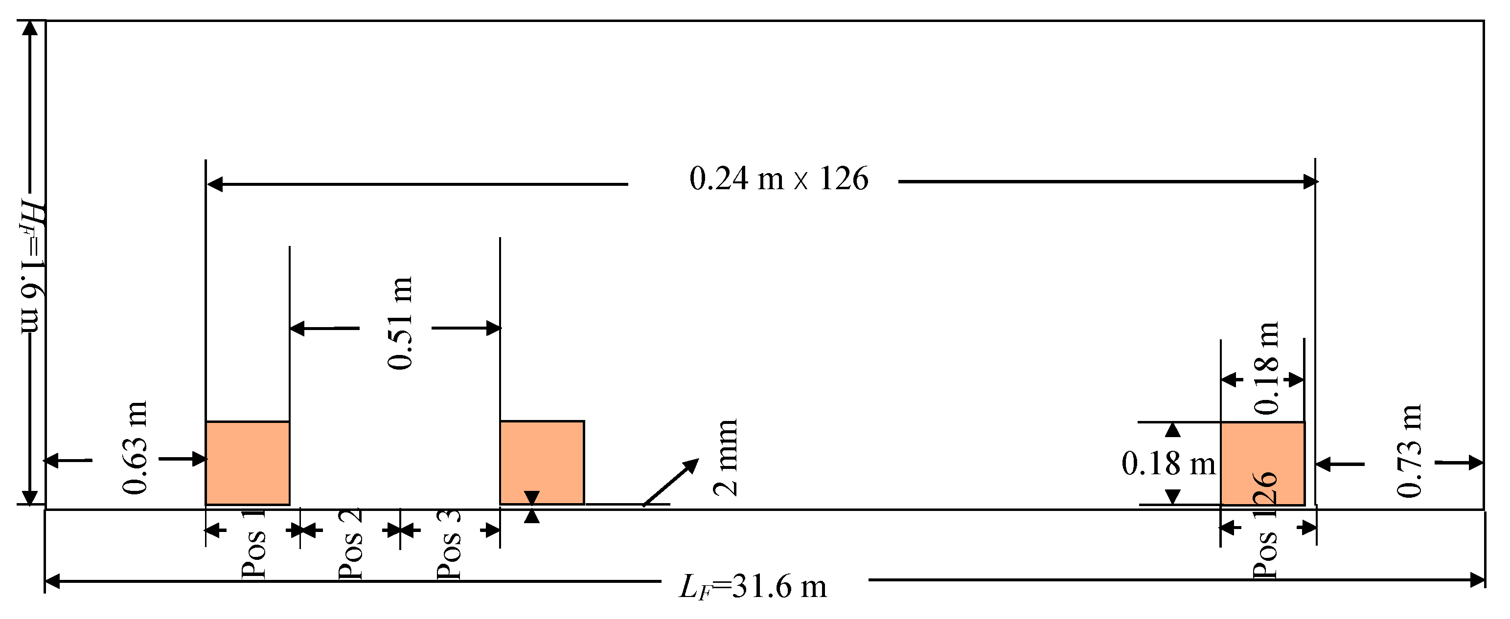
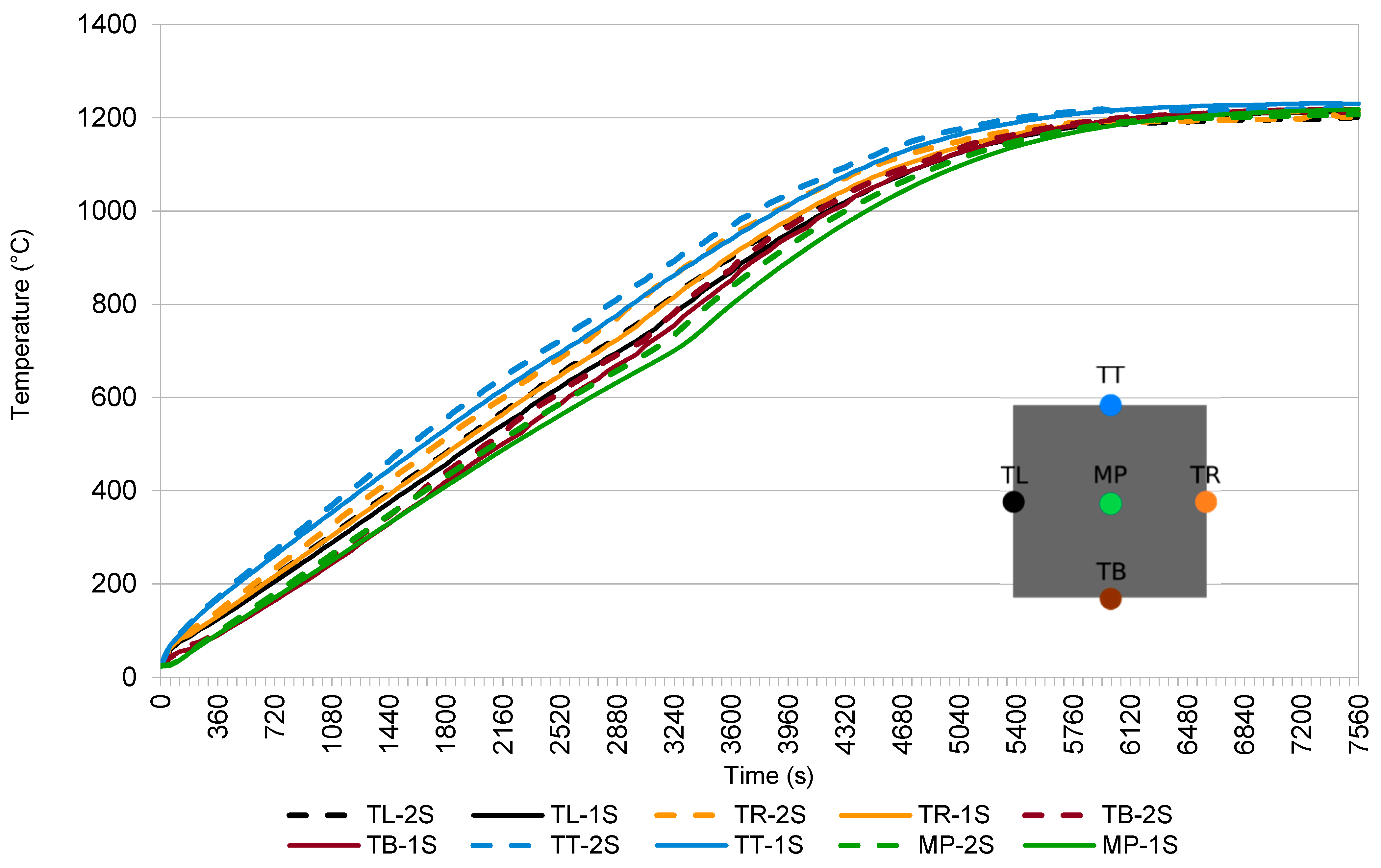
4.3.3. Case 3: Different Spacing between Two Billets

In Case 3, we consider $S_B=0.27 \mathrm{m}$ and $S_B=0.51 \mathrm{m}$, respectively. The cross-section of the furnace with two different spacings between the billets is shown in Figure 9 and Figure 13. The billets stop at each position for 60 s. Additionally, ${10}^6/{\mathrm{m}}^2$ ray densities are used in the Monte Carlo method to calculate the view factor. The results are shown in Figure 14.

Figure 13. The cross-section of the furnace with the billets. Two spaces between each two billets. There are 42 billets in the furnace.

Figure 14. The results of Case 3: the temperature field in 5 representative points of the billets as a function of one (1S) and two (2S) spacings between the billets.

In this case, the temperatures with larger spacing are slightly higher than those with shorter spacing. This is because the billets received more energy from the walls of the furnace.

5. Conclusions

The steel billets in a reheating furnace are simulated by using the LRBFCM. The temperature fields depend on the radiative and convective heat fluxes on the boundaries at different positions in the furnace. The Monte Carlo method is employed to determine the radiative heat flux. To verify the presented model, two comparisons with the reference solution have been made. In the first, a small part of the billet is placed in the middle of a furnace with uniform wall temperatures. The convergence of the results of the view factors with an increasing number of rays is observed. In this way, we were sure that the boundary conditions were correctly implemented. In the second case, the billet is placed close to the bottom, and realistic wall temperatures are applied. The temperature results of the billet in the simulation after 8000 s match perfectly with the reference result.

Three test cases were performed to show the capabilities of this simulation system while using a real reheating furnace environment. These test cases are as follows: a different number of ray densities emitted for calculating the view factors, different stopping time of the billets at each position, and different spacing between two billets, respectively. We obtained the temperature results of the billets for any position and time in the furnace.

Case 1 demonstrates that there is no obvious difference in temperature results when more than ${10}^5/{\mathrm{m}}^2$ ray samples are used in the Monte Carlo method. In the simulations, view factors are calculated once for each position independently of time and we also know from example 5.1 that the magnitude of fluctuations decreases with increasing ray density. Hence, by using the same stopping time at each position, the effect of the ray density may not be so noticeable in the results throughout the simulation. Case 2 demonstrates that a suitable billet stopping time can be found using the described model. Case 3 demonstrates that when a longer distance between each two billets is used, the increase in the temperature is more rapid, especially at the beginning. This simulator can help the steel industry to save energy and optimize productivity. It is extremely complicated to also simulate the temperature of the furnace walls simultaneously. The temperatures of the furnace walls are kept constant in present simulations; however, they would change when a billet enters or leaves the furnace. The presented temperature model of the furnace represents a crucial first step towards optimizing the billets’ quality, furnace productivity, energy, and consumption.

References

- Zhao, J.; Ma, L.; Zayed, M.E.; Elsheikh, A.H.; Li, W.; Yan, Q.; Wang, J. Industrial reheating furnaces: A review of energy efficiency assessments, waste heat recovery potentials, heating process characteristics and perspectives for steel industry. Process Saf. Environ. Prot. 2021, 147, 1209–1228. [Google Scholar] [CrossRef]
- Astolfi, G.; Barboni, L.; Cocchioni, F.; Pepe, C.; Zanoli, S.M. Optimization of a pusher type reheating furnace: An adaptive Model Predictive Control Approach. In Proceedings of the 6th International Symposium on Advanced Control of Industrial Processes, Taipei, Taiwan, 28–31 May 2017. [Google Scholar]
- Harish, J.; Dutta, P. Heat transfer analysis of pusher type reheat furnace. Ironmak. Steelmak. 2005, 32, 151–158. [Google Scholar] [CrossRef]
- Luo, X.C.; Yang, Z. A new approach for estimation of total heat exchange factor in reheating furnace by solving an inverse heat conduction problem. Int. J. Heat Mass Transf. 2017, 112, 1062–1071. [Google Scholar] [CrossRef]
- Kim, J.G.; Huh, K.Y.; Kim, I.T. Three-dimensional analysis of the walking-beam-type slab reheating furnace in hot strip mills. Numer. Heat Transf. Part A Appl. 2000, 38, 589–609. [Google Scholar]
- De Ras, K.; Van de Vijver, R.; Galvita, V.V.; Marin, G.B.; Van Geem, K.M. Carbon capture and utilization in the steel industry: Challenges and opportunities for chemical engineering. Curr. Opin. Chem. Eng. 2019, 26, 81–87. [Google Scholar] [CrossRef]
- Royo, P.; Ferreira, V.J.; López-Sabirón, A.M.; García-Armingol, T.; Ferreira, G. Retrofitting strategies for improving the energy and environmental efficiency in industrial furnaces: A case study in the aluminium sector. Renew. Sustain. Energy Rev. 2018, 82, 1813–1822. [Google Scholar] [CrossRef]
- Zhang, C.; Ishii, T.; Sugiyama, S. Numerical modeling of the thermal performance of regenerative slab reheat furnaces. Numer. Heat Transf. Part A Appl. 1997, 32, 613–631. [Google Scholar] [CrossRef]
- Kim, J.G.; Huh, K.Y. Prediction of transient slab temperature distribution in the re-heating furnace of a walking-beam type for rolling of steel slabs. ISIJ Int. 2000, 40, 1115–1123. [Google Scholar] [CrossRef]
- Hsieh, C.T.; Huang, M.J.; Lee, S.T.; Wang, C.H. Numerical modeling of a walking-beam-type slab reheating furnace. Numer. Heat Transf. Part A Appl. 2008, 53, 966–981. [Google Scholar] [CrossRef]
- Mramor, K.; Vertnik, R.; Šarler, B. Meshless approach to the large-eddy simulation of the continuous casting process. Eng. Anal. Bound. Elem. 2022, 138, 319–338. [Google Scholar] [CrossRef]
- Hanoglu, U.; Šarler, B. Developments towards a multiscale meshless rolling simulation system. Materials 2021, 14, 4277. [Google Scholar] [CrossRef] [PubMed]
- Vuga, G.; Mavrič, B.; Hanoglu, U.; Šarler, B. A hybrid radial basis function-finite difference method for modelling two-dimensional thermo-elasto-plasticity, Part 2: Application to cooling of hot-rolled steel bars on a cooling bed. Eng. Anal. Bound. Elem. 2024, 159, 331–341. [Google Scholar] [CrossRef]
- Lorbiecka, A.Z.; Vertnik, R.; Gjerkeš, H.; Manojlovic, G.; Sencic, B.; Cesar, J.; Šarler, B. Numerical modeling of grain structure in continuous casting of steel. Comput. Mater. Contin. 2009, 8, 195–208. [Google Scholar]
- Mills, A.F.; Coimbra, C.F.M. Basic Heat and Mass Transfer, 3rd ed.; Temporal Publishing, LLC: San Diego, CA, USA, 2015. [Google Scholar]
- Modest, M.F. Radiative Heat Transfer, 3rd ed.; Academic Press: New York, NY, USA, 2013; pp. 365–366. [Google Scholar]
- Jaklič, A.; Vode, F.; Kolenko, T. Online simulation model of the slab-reheating process in a pusher-type furnace. Appl. Therm. Eng. 2007, 27, 1105–1114. [Google Scholar] [CrossRef]
- Šarler, B.; Vertnik, R. Meshfree explicit local radial basis function collocation method for diffusion problems. Comput. Math. Appl. 2006, 51, 1269–1282. [Google Scholar] [CrossRef]
- Ali, I.; Hanoglu, U.; Vertnik, R.; Šarler, B. Assessment of Local Radial Basis Function Collocation Method for Diffusion Problems Structured with Multiquadrics and Polyharmonic Splines. Math. Comput. Appl. 2024, 29, 23. [Google Scholar] [CrossRef]
- Ansys Fluent Academic Research Release 18.2: Fluid Simulation Software; ANSYS: Canonsburg, PA, USA. Available online: https://www.ansys.com/products/fluids/ansys-fluent (accessed on 29 September 2023).
- Saunders, N.; Guo, U.K.Z.; Li, X.; Miodownik, A.P.; Schille, J.P. Using JMatPro to model materials properties and behavior. JOM 2003, 55, 60–65. [Google Scholar] [CrossRef]
Disclaimer/Publisher’s Note: The statements, opinions and data contained in all publications are solely those of the individual author(s) and contributor(s) and not of MDPI and/or the editor(s). MDPI and/or the editor(s) disclaim responsibility for any injury to people or property resulting from any ideas, methods, instructions or products referred to in the content. |
© 2024 by the authors. Licensee MDPI, Basel, Switzerland. This article is an open access article distributed under the terms and conditions of the Creative Commons Attribution (CC BY) license (https://creativecommons.org/licenses/by/4.0/).