Abstract
The primary purpose of this work is to provide a new fractional boundary element method (BEM) formulation to solve thermal stress wave propagation problems in anisotropic materials. In the Laplace domain, the fundamental solutions to the governing equations can be identified. Then, the boundary integral equations are constructed. The Caputo fractional time derivative was used in the formulation of the considered heat conduction equation. The three-block splitting (TBS) iteration approach was used to solve the resulting BEM linear systems, resulting in fewer iterations and less CPU time. The new TBS iteration method converges rapidly and does not involve complicated computations; it performs better than the two-dimensional double successive projection method (2D-DSPM) and modified symmetric successive overrelaxation (MSSOR) for solving the resultant BEM linear system. We only studied a special case of our model to compare our findings to those of other articles in the literature. Because the BEM results are so consistent with the finite element method (FEM) findings, the numerical results demonstrate the validity, accuracy, and efficiency of our proposed BEM formulation for solving three-dimensional thermal stress wave propagation problems in anisotropic materials.
1. Introduction
Within the discipline of continuum mechanics, thermoelasticity studies the relationship between mechanical memory and thermodynamics in the behavior of solid bodies. There are various options for doing this. The most general method is to try to put thermodynamic constraints on the constitutive equations, with deformation and temperature as dependent variables [1,2,3]. In some materials, these constraints are so specific that, among the infinite ways of coupling mechanics and thermodynamics, certain closed sets of equations can be obtained that characterize the unknown driving forces of the coupled field. The most typical sets of linked equations appear to be very simplified versions of what can be obtained using a more generic approach [4]. However, when a non-quadratic elastic energy function is considered, the simplifying feature required to distinguish one theory from others may not always be reduced to the property of meeting a set of equilibrium equations and a temperature equation [5,6].
Fractional calculus is the study of the properties and results of the derivative of a function of order . It provides tools to understand phenomena and processes that evolve in time in a more accurate way than those offered by classical integral and differential calculus, considering long memories in their internal evolution [7,8]. Moreover, fractional calculus is naturally used to model processes with unique and non-local effects, which are considered highly complex. Indeed, phenomena described by models based on non-integer order integrals and derivatives have attracted the attention of the scientific community and have been applied in several areas not only as mathematical models but also as theoretical tools for the study of other physical phenomena [9,10,11]. The rapid development of computational and theoretical techniques to efficiently deal with mathematical models based on fractional calculus, as well as the success of these models in solving mathematical problems, has naturally motivated several scientific researchers to investigate the potential of these models in solving various engineering problems, with positive and significant complex effects. Consequently, fractional calculus models began to spread into distinct traditional fields of engineering like control and power systems, becoming a major topic of investigation in all other fields. Fractional calculus is undoubtedly a very valuable tool for the study of complex media and has a considerable impact in many different fields, both theoretical and experimental. Nevertheless, the physico-mathematical aspect perceived in the theory of rate-type constitutive models for the specific formulation of the stress tensor in linear and nonlinear thermoelasticity cannot be completely established until the physical meaning of the fractional order and the causality principle are well understood [12,13].
Another important topic in modern engineering is anisotropy. Anisotropic materials comprise most materials in a solid-state body. Beams and plates in a cross-section can be, and in some cases must be, modeled as anisotropic. It is difficult to define the category of anisotropic materials in a convenient manner. However, this term is usually used to describe materials that are neither isotropic nor transversely isotropic. Anisotropy occurs in materials such as single crystals, rolled pentagonal structures, etc. Anisotropic materials have 4 elastic constants, so there are 21 independent elastic constants for general materials. The permissible anisotropic qualities are determined by the symmetry of the coefficients of the elastic component in the formulation of the deformation equilibrium equation [14,15]. If symmetry conditions on each component’s elastic coefficients are considered, then the strain energy function can identify numerous types of anisotropy and their associations [16,17].
The concept of generalized thermoelasticity theories was introduced separately in 1972 and 1970. The reasons for generalizing the theory originated from the fact that the mathematical opponent of the simple theory was faced while solving the problem of the relative size of the thermal field and the premise upon which the theory was founded [18,19]. The mechanical portion of the thermodynamic surface of elastic materials, as well as the first full set of thermodynamic balances that offer motion equations, extended Hooke’s law, the energy equation, and other results, serves as the foundation for classical thermoelasticity theory [20,21,22]. The thermal field enters only the second rank of the dissipation functional through entropy and entropy balance, which is determined by the dissipation functional’s local extreme. To address the issue, a full thermodynamic functional incorporating the thermal field was constructed. The presence of the thermodynamic principle and the entire thermodynamic functional in characterizing the thermal behavior of a solid has been discussed [23,24].
To address the first problem in the classical thermo-elasticity (CTE) theory proposed by Duhamel [25] and Neumann [26], which predicts two occurrences that contradict empirical facts, Biot [27] proposed the classical coupled thermo-elasticity (CCTE) theory. Most methods for overcoming the classical theory’s unwanted prediction are based on the non-Fourier effect. Lord and Shulman [28] proposed an extended thermoelasticity (ETE) theory with a single relaxation time. Green and Lindsay [29] proposed the temperature rate-dependent thermoelasticity (TRDTE) theory, which incorporates temperature rate as a constitutive variable. Green and Naghdi [30,31] made substantial theoretical advances in the field, developing three models for the generalized thermoelasticity of homogeneous isotropic materials. Chen and Gurtin [32] and Chen et al. [33,34] proposed heat conduction theory based on conductive and thermodynamic temperatures. Quintanilla [35] conducted extensive research on the two-temperature thermoelasticity theory. Youssef [36] introduced the two-temperature generalized thermoelasticity theory, which has been applied to solve several engineering problems [37,38,39,40].
The thermoelastic problem has been studied since the fundamental equations that govern it were deduced. Problems involving a heating source and with or without external forces have been the subject of many analyses. It is difficult to identify the analytical solution for such problems; thus, several numerical methods exist for estimating solutions to these problems [41,42,43,44,45]. In recent years, new methods have proven to be useful when used to thermoelasticity problems [46,47,48,49]. All these methods are based on solid mathematical principles and can be automated; however, they often require software to achieve the result. Because not all natural phenomena can be characterized by integer-order partial differential equations, some are represented by fractional partial differential equations (FPDEs). Most fractional differential equations do not have explicit analytical solutions; hence, several researchers have devised numerical solution methodologies for time-fractional partial differential equations (TFPDEs). The boundary element method (BEM) is a numerical technique for solving partial differential equations (PDEs) with time-fractional order. This technique combines boundary integral equations with numerical approximation of boundary integrals. These equations can be obtained from the fundamental solutions to PDEs’ differential operators. The most significant advantage of the BEM is that the needed discretization of the domain is one less than that of other numerical approaches. It has significant advantages over traditional methods like the finite element method (FEM) and the finite difference method (FDM). One of the key advantages of the BEM is that it is a boundary-only approach, which means that only the issue’s boundary must be discretized, resulting in a one-dimensional problem [50,51,52]. A two-dimensional problem, for example, requires two dimensions of discretization in the FEM or FDM, whereas the BEM just requires one. This is useful for boundary layer problems, which demand tighter grids in locations with large gradients. The BEM has an even greater advantage for problems with infinite or semi-infinite domains, as it is usually necessary to truncate the domain in the FEM or FDM and introduce artificial boundaries with associated treatments such as adding boundary conditions, whereas this is not the case with the BEM because only the boundary is discretized. Domain discretization in the FEM or FDM also requires mesh production, which can frequently be challenging and a time-consuming task [53,54,55]. This is especially difficult for complex domains or problems whose domain geometry changes over time. With recent computer improvements, numerical approaches based on boundary integral equations have garnered significant attention due to their success in addressing a variety of two-dimensional issues. The boundary element method (BEM) is a popular numerical technique that has applications in a variety of engineering fields, including fluid mechanics, magnetohydrodynamics, and electrodynamics. Recent advances in the BEM have made it possible to apply this method to increasingly complex issues, such as multi-regions [56,57,58].
Although the boundary element method (BEM) is widely acknowledged for its best-use scenario in tackling high-dimensional issues, one impediment remains to be overcome to make it more accessible and easier to use [59,60,61]. This impediment is the need for remedies for low-frequency situations in prospective issues; otherwise, numerical instability will be introduced. In recent decades, several initiatives have been made to address this issue, with most of them focused on the concept of transitioning from the original domains to new ones [62,63,64]. However, those existing translation methods either rely on operator solutions or generate several integral types for a single state variable. As a result, in practice, they continue to make BEM deployment more challenging. As a result, it is important and meaningful to develop a transformation method that keeps the benefits of simple boundary-type methods while addressing the numerical instability difficulties of low-frequency instances [65,66,67,68]. The scaled coordinate transformation (SCT) is purely a mathematical operation that, like the original coordinate transformation, requires only discretization on the structure’s surface while remaining analytical in the radial direction, eliminating the need for half-domain discretization and second derivative computations. The scaled coordinate transformation boundary element method (SCTBEM) uses the same integral types and operations on discretized boundary elements as the conventional BEM. However, with the newly devised coordinate transformation, there is no need to be concerned about low-frequency situations in prospective difficulties. Numerical findings demonstrate that the SCTBEM is robust and accurate, even when dealing with very low wave numbers or very huge structures. In addition, the SCTBEM provides a research topic that is not confined to the BEM. Coordinate transformation is a purely mathematical technique that modifies domain integrals in potential problems while leaving boundary integrals untouched. As a result, the SCTBEM can be used for other domain-type methods that use integrals for state variables that are comparable in form [68,69].
Three-block splitting (TBS) is an FFT-based iterative method for solving the three-dimensional time–domain boundary integral equation of the wave equation that is formulated with respect to the boundary magnetic field. In this equation, the time derivative of the boundary magnetic field appears with minus sign, and thus, it has the time-delayed exponential integrator (TDEI) type. The TBS approximately splits this boundary integral equation into three blocks with respect to the wave number components. The convergence of the TBS iteration depends on the value of the time step. For a large time step, the TBS iteration does not converge. To overcome this difficulty, the TBS iteration is applied first with a coarse time step for a few iterations, and then it is applied with the original time step [70].
In the present paper, we investigated the fundamental solutions of fractional order coupled with anisotropic thermoelasticity in the Laplace domain. The fractional boundary element technique was then formulated using a suitable reciprocal connection to solve the considered problem. The boundary was discretized at the collocation nodes. The original problem’s boundary integral equations at these collocation points were then solved using the point collocation method. Finally, we presented the results of the suggested BEM model, which better explained our formulation for 3D thermal stress wave propagation in anisotropic materials.
2. Formulation of the Problem
Based on Cattaneo [71] and Vernotte’s [72,73] heat conduction equation and definition of the Caputo derivative, Sherief et al. [74] proposed the following fractional heat conduction equation:
In Cartesian coordinates, the governing equations for 3D thermal stress wave propagation in anisotropic materials are [28]
where
Now, we assume the following conditions:
By applying Equation (4), the traction vector can be represented as follows:
3. Boundary Element Implementation
Function has the following Laplace transform:
Via the application of the Laplace transform to Equations (2)–(4), we obtain
We now present the vectors of displacement and body force as follows:
To obtain the fundamental solutions in the Laplace transform domain, we consider the following two cases:
3.1. Case 1:
Based on [75], we obtain
where are the solutions of the following characteristic equation:
Equation (21) has the following solution:
which can be written using the Helmholtz equation as follows:
Thus, Equations and (24) yield
and
The Laplace transform was successfully applied to the traction vector to yield (see Appendix A)
3.2. Case 2:
In the absence of a heat source, we find
where
Now, we establish that the temperature in Case 2 is proportional to the displacement in Case 1 as follows:
where
The traction vector is then obtained in a manner like that used in Case 1
where
Sherief et al. [74] introduced the following reciprocal relation:
To describe the displacement and temperature integral equation with respect to the specified functions , fundamental solutions and their values on , we consider Case 1 () and Case 2 () below.
For case 1, Equation becomes
where
For Case II, Equation (41) can be expressed as
Equation (42) can be solved by using the inverse Laplace transform as follows:
we arrive at
where
The solution of (44) yields
Where Mittag–Leffler function is defined as follows [76]:
Similarly, from Equation (43), we obtain
where
By solving Equation (48), we obtain
Consider the of (46) and of (50). Thus, we have
The resulting linear systems were solved using the iteration approach of three-block splitting (TBS) [77].
Figure 1 shows the proposed BEM algorithm flowchart.
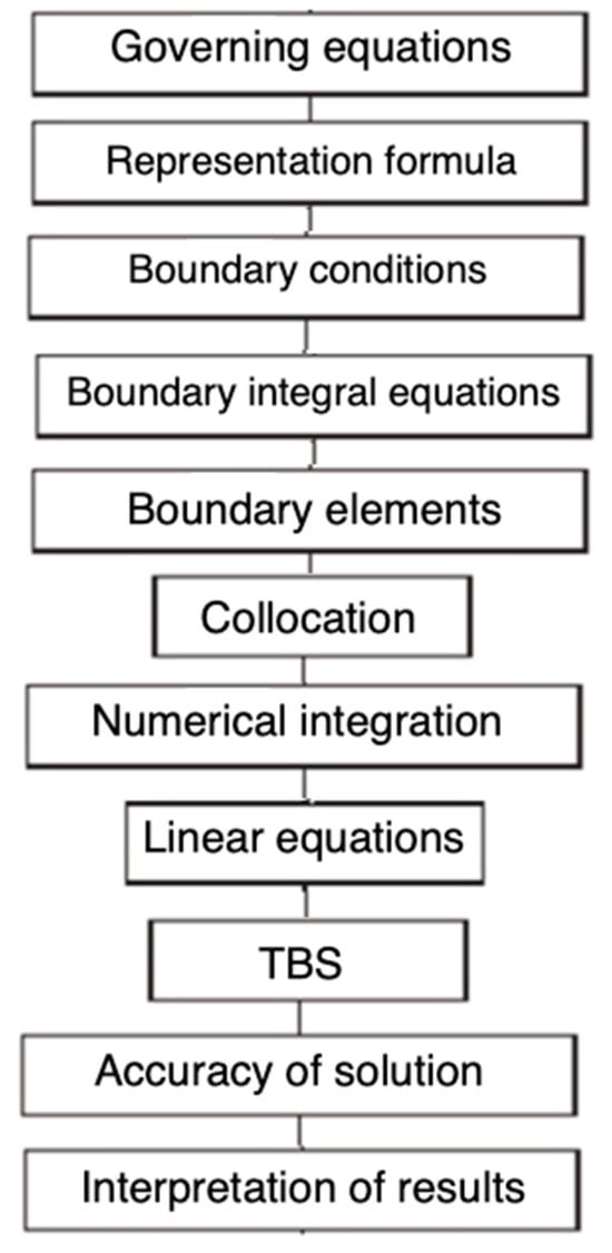
Figure 1.
Flowchart of the considered BEM model.
This study focuses on the computational domain, which has 40 boundary nodes and 81 interior nodes, as indicated in Figure 2.
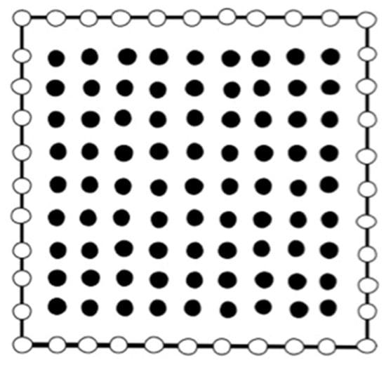
Figure 2.
BEM model of the considered problem.
4. Numerical Results and Discussion
To exemplify the numerical findings provided by the proposed methodology, an anisotropic alumina was studied, which had the following properties [14]:
Anisotropic elasticity tensor
Thermal moduli
Figure 3 shows the distribution of thermal stress wave propagation throughout the -axis for various fractional parameter values. The figure shows that the thermal stress waves grow nonlinearly at , then decline linearly and quickly converge to zero at . It is also recognized that when fractional parame increases, so does . This figure depicts the way the fractional parameter affects the propagation of the thermal stress wave in anisotropic materials.
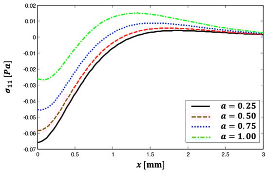
Figure 3.
The distribution of thermal stress wave propagation throughout the -axis for various fractional parameter values.
Figure 4 shows the distribution of thermal stress wave propagation throughout the -axis for various fractional parameter values. The image shows that all curves begin at and rise nonlinearly until they reach a maximum at . The function reduces nonlinearly until it reaches a minimal value at . The curves then expand linearly until they meet at approximately . It is also noted that diminishes with an increase in fractional parameter a. The figure depicts the way the fractional parameter affects the propagation of the thermal stress wave in anisotropic materials.
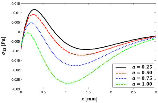
Figure 4.
The distribution of thermal stress wave propagation throughout the -axis for various fractional parameter values.
Figure 5 shows the distribution of thermal stress wave propagation throughout the x-axis for various fractional parameter values. This graphic shows that all curves begin at and subsequently drop nonlinearly until they reach a minimum at . Then, they increase nonlinearly until they meet at around . It is also noted that when the fractional parameter grows, so does . This figure depicts the way the fractional parameter affects the propagation of the thermal stress wave in anisotropic materials.
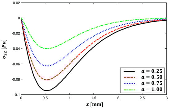
Figure 5.
The distribution of thermal stress wave propagation throughout the -axis for various fractional parameter values.
Figure 6 shows the distribution of thermal stress wave propagation throughout the x-axis for various fractional parameter values. This graphic shows that all curves begin with a maximum value at , and as the distance increases, these values decrease to practically zero at . Additionally, as the fractional parameter grows, so does . This figure depicts the way the fractional parameter affects the propagation of the thermal stress wave in anisotropic materials.
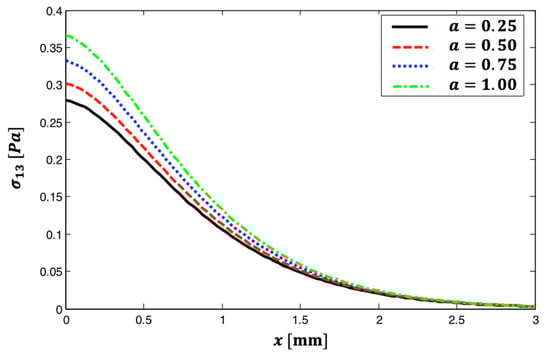
Figure 6.
The distribution of thermal stress wave propagation throughout the -axis for various fractional parameter values.
Figure 7 shows the distribution of thermal stress wave propagation throughout the -axis for various fractional parameter values. This image shows that all curves decrease nonlinearly until they reach a minimal value at , after which, climbs nonlinearly to approach zero at . Additionally, as the fractional parameter increases, diminishes. The fractional parameter has a substantial impact on thermal stress wave propagation in thermoelastic materials, as illustrated in this figure.
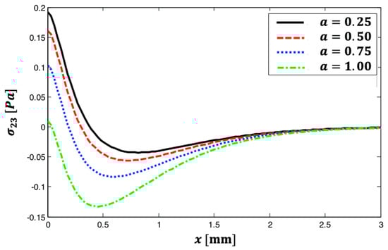
Figure 7.
The distribution of thermal stress wave propagation throughout the -axis for various fractional parameter values.
Figure 8 shows the distribution of thermal stress wave propagation throughout the x-axis for various fractional parameter values. This image shows that the curves begin with separate values at , then change and coincide until they reach zero at . It is also noted that when the fractional parameter grows, so does . This graphic illustrates how the fractional parameter affects thermal stress wave propagation in thermoelastic materials.
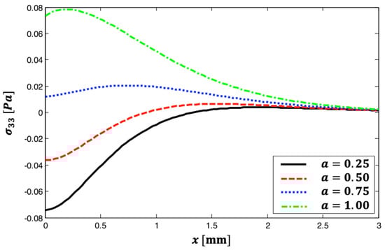
Figure 8.
The distribution of thermal stress wave propagation throughout the -axis for various fractional parameter values.
For validation, we used a particular example of our model and compared our BEM results to Marin et al.’s FEM results [78] and Sharifi’s analytical results [79].
Figure 9, Figure 10 and Figure 11 depict the distributions of thermal stress and waves propagating throughout the -axis using BEM, FEM [78] and analytical [79] models. These figures show that the BEM is in excellent agreement with the FEM and analytical methods demonstrating the validity and accuracy of our proposed technique. Matlab R2022a was utilized to generate the computation results for the problem at hand. The proposed fractional boundary element technique in this study is applicable to a wide range of thermal stress wave propagation problems in thermoelastic materials.
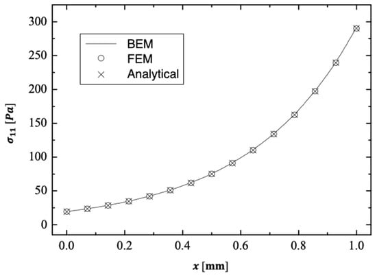
Figure 9.
The distribution of thermal stress wave propagation throughout the -axis using BEM, FEM and analytical methods.
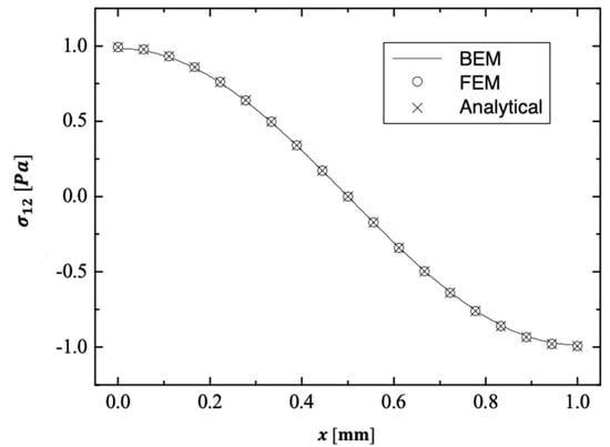
Figure 10.
The distribution of thermal stress wave propagation throughout the -axis using BEM, FEM and analytical methods.
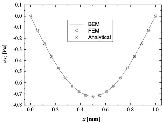
Figure 11.
The distribution of thermal stress wave propagation throughout the -axis using BEM, FEM and analytical methods.
Table 1 displays the CPU time and iteration count for the two-dimensional double successive projection method (2D-DSPM) of Jing and Huang [80], modified symmetric successive overrelaxation (MSSOR) of Darvishi and Hessari [81] and three-block splitting (TBS) of Li et al. [77] iterative methods at each discretization level, with equation numbers in brackets. This table demonstrates that the TBS strategy exceeds both the 2D-DSPM and MSSOR methods.

Table 1.
CPU timings and iterations for different iterative methods.
Table 2 compares the computational requirements for modeling thermal stress wave propagation problems in anisotropic materials using current BEM and FEM approaches [78]. This table demonstrates the efficacy of our proposed BEM approach.
Table 2.
Study of computational power requirements for modeling thermal stress wave propagation problems in anisotropic materials utilizing current BEM and FEM.
5. Conclusions
The primary goal of this paper was to present a novel fractional boundary element method (BEM) formulation for solving thermal stress wave propagation problems in anisotropic materials. In the Laplace domain, the fundamental solutions to the governing equations could be found. The boundary integral equations were then built. The heat conduction equation under consideration was formulated using the Caputo fractional time derivative. The resulting BEM linear systems were solved using the three-block splitting (TBS) iteration strategy, which required fewer iterations and consumed less CPU time. The new TBS iteration approach converged quickly and did not require complex computations. It outperformed the two-dimensional double successive projection method (2D-DSPM) and modified symmetric successive overrelaxation (MSSOR) in solving the resultant BEM linear system. We only looked at one specific scenario of our model to compare our results to those of other publications in the literature. Because the BEM results were so compatible with the finite element method (FEM) and analytical findings, the numerical results showed that our proposed BEM formulation was valid, accurate, and efficient in handling three-dimensional thermal stress wave propagation problems in anisotropic materials. The current research has several applications, including nuclear physical science, biophysics, geothermal engineering, pressure vessels, econophysics, biochemistry, robotics and control theory, food engineering, signal and image processing, aviation, electronics, and many more.
Author Contributions
Conceptualization, M.A.F.; Methodology, M.A.F.; Software, M.A.F.; Validation, M.A.F.; Formal analysis, M.A.F.; Investigation, M.A.F.; Resources, M.A.F. and M.T.; Data curation, M.A.F.; Writing—original draft, M.A.F. and M.T.; Writing—review & editing, M.A.F. and M.T. All authors have read and agreed to the published version of the manuscript.
Funding
This research received no external funding.
Data Availability Statement
All data generated or analyzed during this study are included in this published article.
Conflicts of Interest
The authors declare no conflicts of interest.
Nomenclature
| Coefficients of thermal expansion | |
| thermal moduli | |
| Kronecker delta | |
| Strains | |
| Stress | |
| Time | |
| Fractional-order parameter | |
| Elastic constants | |
| Specific heat at constant strain | |
| boundary | |
| dilatation | |
| Body force vector | |
| Non-Gaussian temporal profile | |
| Total energy intensity | |
| Thermal conductivity | |
| Outward normal components | |
| Heat source intensity | |
| Irradiated surface absorptivity | |
| radial distance | |
| Temperature | |
| Temperature fundamental solutions | |
| Reference temperature | |
| Laser pulse time characteristic | |
| Displacement vector | |
| Displacement fundamental solutions | |
Appendix A. Laplace Transform Implementation
The traction vector on can be expressed as
The Laplace transform was successfully applied to the traction vector (A1) to yield
The derivative of Equation (A3) gives
where
and
Equation (A4) may be expressed as
where
Thus, using Equations (A2) and (A7), we obtain
Appendix B. Helmholtz Theorem Implementation
The Helmholtz theorem is applied to vectors and to obtain
where the potentials , , , and satisfy the following relations:
The Helmholtz decomposition theorem is used to determine
References
- Ezzat, M.; Zakaria, M.; Shaker, O.; Barakat, F. State space formulation to viscoelastic fluid flow of magnetohydrodynamic free convection through a porous medium. Acta Mech. 1996, 119, 147–164. [Google Scholar] [CrossRef]
- Ezzat, M.A. Free convection effects on perfectly conducting fluid. Int. J. Eng. Sci. 2001, 39, 799–819. [Google Scholar] [CrossRef]
- Fahmy, M.A. Thermoelastic stresses in a rotating non-homogeneous aniso-tropic body. Numer. Heat Transf. Part A 2008, 53, 1001–1011. [Google Scholar] [CrossRef]
- Abouelregal, A.E.; Mohammed, W.W. Effects of nonlocal thermoelasticity on nanoscale beams based on couple stress theory. Math. Methods Appl. Sci. 2020. [Google Scholar] [CrossRef]
- Othman, M.I.A.; Abd-Elaziz, E.M. Dual-phase-lag model on micropolar thermoelastic rotating medium under the effect of thermal load due to laser pulse. Indian J. Phys. 2020, 94, 999–1008. [Google Scholar] [CrossRef]
- Othman, M.I.A.; Zidan, M.E.M.; Mohamed, I.E.A. Dual-phase-lag model on thermo-microstretch elastic solid under the effect of initial stress and temperature-dependent. Steel Compos. Struct. 2021, 38, 355–363. [Google Scholar]
- Bagley, R.L.; Torvik, P.J. On the fractional calculus model of viscoelastic behavior. J. Rheol. 1986, 30, 133–155. [Google Scholar] [CrossRef]
- Machado, J.A.T. Analysis and design of fractional-order digital control systems. SAMS J. Syst. Anal. Model. Simul. 1997, 27, 107–122. [Google Scholar]
- Oldham, K.B.; Spanier, J. The Fractional Calculus: Theory and Applications of Differentiation and Integration to Arbitrary Order, 1st ed.; Dover Publication: Mineola, NY, USA, 2006; Volume 111, pp. 1–64. [Google Scholar]
- Kilbas, A.A.; Srivastava, H.M.; Trujillo, J.J. Theory and Applications of Fractional Differential Equations, 1st ed.; Elsevier Science: Amsterdam, The Netherlands, 2006; Volume 204, pp. 449–463. [Google Scholar]
- Sabatier, J.; Agrawal, O.P.; Machado, J.A.T. Advances in Fractional Calculus: Theoretical Developments and Applications in Physics and Engineering, 1st ed.; Springer: Dordrecht, The Netherlands, 2007; Volume 1, pp. 169–302. [Google Scholar]
- Wang, J.L.; Li, H.F. Surpassing the fractional derivative: Concept of the memory-dependent derivative. Comput. Math. Appl. 2011, 62, 1562–1567. [Google Scholar] [CrossRef]
- Yu, Y.J.; Zhao, L.J. Fractional thermoelasticity revisited with new definitions of fractional derivative. Eur. J. Mech.—A/Solids 2020, 84, 104043. [Google Scholar] [CrossRef]
- Shiah, Y.C.; Tuan, N.A.; Hematiyan, M.R. Direct transformation of the volume integral in the boundary integral equation for treating three-dimensional steady-state anisotropic thermoelasticity involving volume heat source. Int. J. Solids Struct. 2018, 143, 287–297. [Google Scholar] [CrossRef]
- Fahmy, M.A. Boundary element algorithm for nonlinear modeling and simulation of three temperature anisotropic generalized micropolar piezothermoelasticity with memory-dependent derivative. Int. J. Appl. Mech. 2020, 12, 2050027. [Google Scholar] [CrossRef]
- Fahmy, M.A. Boundary element modeling of fractional nonlinear generalized photothermal stress wave propagation problems in FG anisotropic smart semiconductors. Eng. Anal. Bound. Elem. 2022, 134, 665–679. [Google Scholar] [CrossRef]
- Fahmy, M.A.; Shaw, S.; Mondal, S.; Abouelregal, A.E.; Lotfy, K.; Kudinov, I.A.; Soliman, A.H. Boundary Element Modeling for Simulation and Optimization of Three-Temperature Anisotropic Micropolar Magneto-thermoviscoelastic Problems in Porous Smart Structures Using NURBS and Genetic Algorithm. Int. J. Thermophys. 2021, 42, 29. [Google Scholar] [CrossRef]
- Othman, M.I.A.; Atwa, S.Y.; Farouk, R.M. Generalized magneto-thermoviscoelastic plane waves under the effect of rotation without energy dissipation. Int. J. Eng. Sci. 2008, 46, 639–653. [Google Scholar] [CrossRef]
- Othman, M.I.A.; Song, Y. Effect of rotation on plane waves of generalized electro magneto-thermoviscoelasticity with two relaxation times. Appl. Math. Model. 2008, 32, 811–825. [Google Scholar] [CrossRef]
- Ezzat, M.A.; Awad, E.S. Micropolar generalized magneto-thermoelasticity with modified Ohm’s and Fourier’s laws. J. Math. Anal. Appl. 2009, 353, 99–113. [Google Scholar] [CrossRef]
- Ezzat, M.A.; Youssef, H.M. Generalized magneto-thermoelasticity in a perfectly conducting medium. Int. J. Solids Struct. 2005, 42, 6319–6334. [Google Scholar] [CrossRef]
- Othman, M.I.A.; Eraki, E.E.M. Effect of gravity on generalized thermoelastic diffusion due to laser pulse using dual-phase-lag model. Multidiscip. Model. Mater. Struct. 2018, 14, 457–481. [Google Scholar] [CrossRef]
- Fahmy, M.A. A Nonlinear Fractional BEM Model for Magneto-Thermo-Visco-Elastic Ultrasound Waves in Temperature-Dependent FGA Rotating Granular Plates. Fractal Fract. 2023, 7, 214. [Google Scholar] [CrossRef]
- Fahmy, M.A. A New Boundary Element Strategy for Modeling and Simulation of Three Temperatures Nonlinear Generalized Micropolar-Magneto-Thermoelastic Wave Propagation Problems in FGA Structures. Eng. Anal. Bound. Elem. 2019, 108, 192–200. [Google Scholar] [CrossRef]
- Duhamel, J. Some memoire sur les phenomenes thermo-mechanique. J. L’école Polytech. 1837, 15, 1–57. [Google Scholar]
- Neumann, F. Vorlesungen Uber die Theorie der Elasticitat; Meyer: Brestau, Germany, 1885. [Google Scholar]
- Biot, M. Thermoelasticity and irreversible thermo-dynamics. J. Appl. Phys. 1956, 27, 249–253. [Google Scholar] [CrossRef]
- Lord, H.W.; Shulman, Y. A generalized dynamical theory of thermoelasticity. J. Mech. Phys. Solids 1967, 15, 299–309. [Google Scholar] [CrossRef]
- Green, A.E.; Lindsay, K.A. Thermoelasticity. J. Elast. 1972, 2, 1–7. [Google Scholar] [CrossRef]
- Green, A.E.; Naghdi, P.M. On undamped heat waves in an elastic solid. J. Therm. Stress. 1992, 15, 253–264. [Google Scholar] [CrossRef]
- Green, A.E.; Naghdi, P.M. Thermoelasticity without energy dissipation. J. Elast. 1993, 31, 189–208. [Google Scholar] [CrossRef]
- Chen, P.J.; Gurtin, M.E. On a theory of heat conduction involving two temperatures. Z. Angew. Math. Phys. ZAMP 1968, 19, 614–627. [Google Scholar] [CrossRef]
- Chen, P.J.; Gurtin, M.E.; Williams, W.O. A note on non-simple heat conduction. Z. Angew. Math. Phys. ZAMP 1968, 19, 969–970. [Google Scholar] [CrossRef]
- Chen, P.J.; Gurtin, M.E.; Williams, W.O. On the thermodynamics of non-simple elastic materials with two temperatures. Z. Angew. Math. Phys. ZAMP 1969, 20, 107–112. [Google Scholar] [CrossRef]
- Quintanilla, R. On existence, structural stability, convergence and spatial behavior in thermoelasticity with two-temperatures. Acta Mech. 2004, 168, 61–73. [Google Scholar] [CrossRef]
- Youssef, H.M. Theory of two-temperature generalized thermoelasticity. IMA J. Appl. Math. 2006, 71, 383–390. [Google Scholar] [CrossRef]
- Youssef, H.M.; Al-Lehaibi, E.A. State-space approach of two-temperature generalized thermoelasticity of one dimensional problem. Int. J. Solids Struct. 2007, 44, 1550–1562. [Google Scholar] [CrossRef]
- Bassiouny, E.; Youssef, H.M. Two-temperature generalized thermopiezoelasticity of finite rod subjected to different types of thermal loading. J. Therm. Stress. 2008, 31, 233–245. [Google Scholar] [CrossRef]
- Youssef, H.M. Two-dimensional problem of two-temperature generalized thermoelastic half-space subjected to ramp-type heating. Comput. Math. Model. 2008, 19, 201–216. [Google Scholar] [CrossRef]
- Fahmy, M.A. Shape design sensitivity and optimization for two-temperature generalized magneto-thermoelastic problems using time-domain DRBEM. J. Therm. Stress. 2018, 41, 119–138. [Google Scholar] [CrossRef]
- Rizzo, F.J.; Shippy, D.J. An advanced boundary integral equation method for three-dimensional thermoelasticity. Int. J. Numer. Methods Eng. 1977, 11, 1753–1768. [Google Scholar] [CrossRef]
- Brebbia, C.A. The Boundary Element Method for Engineers; Pentech Press: London, UK, 1978. [Google Scholar]
- Brebbia, C.A.; Walker, S. Boundary Element Method Techniques in Engineering; Newness-Butterworths: London, UK, 1980. [Google Scholar]
- Banerjee, P.K.; Butterfield, R. Boundary Element Methods in Engineering Science; McGraw-Hill: London, UK, 1981. [Google Scholar]
- Fenner, R.T. Boundary element for stress problems. In Seminar on Finite Elements or Boundary Elements; Institution of Mechanical Engineers: London, UK, 1982. [Google Scholar]
- Brebbia, C.A.; Tells, J.C.F.; Wrobel, L.C. Boundary Element Techniques: Theory and Applications in Engineering; Springer: Heidelberg, Germany, 1984. [Google Scholar]
- Sladek, V.; Sladek, J. Boundary integral equation method in two-dimensional thermoelasticity. Eng. Anal. 1984, 1, 135–148. [Google Scholar] [CrossRef]
- Sladek, V.; Sladek, J. Boundary integral equation method in thermoelasticity Part III: Uncoupled thermoelasticity. Appl. Math. Model. 1984, 8, 413–418. [Google Scholar] [CrossRef]
- Cruse, T.A.; Rizzo, F.J. Boundary integral equation methods-computational applications. In Applied Mechanics, Proceedings of the ASME Conference on Boundary Integral Equation Methods; ASME: New York, NY, USA, 1985; pp. 118–123. [Google Scholar]
- Cao, G.; Yu, B.; Chen, L.; Yao, W. Isogeometric dual reciprocity BEM for solving non-Fourier transient heat transfer problems in FGMs with uncertainty analysis. Int. J. Heat Mass Transf. 2022, 203, 123783. [Google Scholar] [CrossRef]
- Sladek, J.; Sladek, V.; Markechova, I. Boundary element method analysis of stationary thermoelasticity problems in non-homogeneous media. Int. J. Numer. Methods Eng. 1990, 30, 505–516. [Google Scholar] [CrossRef]
- Zhang, S.; Yu, B.; Chen, L. Non-iterative reconstruction of time-domain sound pressure and rapid prediction of large-scale sound field based on IG-DRBEM and POD-RBF. J. Sound Vib. 2024, 573, 118226. [Google Scholar] [CrossRef]
- Tanaka, M.; Matsumoto, T.; Moradi, M. Application of boundary element method to 3-D problems of coupled thermoelasticity. Eng. Anal. Boundary. Elem. 1995, 16, 297–303. [Google Scholar] [CrossRef]
- Ang, W.T.; Clements, D.L.; Cooke, T. A Complex Variable Boundary Element Method for a Class of Boundary Value Problems in Anisotropic Thermoelasticity. Int. J. Comput. Math. 1999, 70, 571–586. [Google Scholar] [CrossRef]
- Shiah, Y.C.; Tan, C.L. Exact boundary integral transformation of the thermoelastic domain integral in BEM for general 2D anisotropic elasticity. Comput. Mech. 1999, 23, 87–96. [Google Scholar] [CrossRef]
- Kogl, M.; Gaul, L. A boundary element method for anisotropic coupled thermoelasticity. Arch. Appl. Math. 2003, 73, 377–398. [Google Scholar]
- El-Naggar, A.M.; Abd-Alla, A.M.; Fahmy, M.A. The propagation of thermal stresses in an infinite elastic slab. Appl. Math. Comput. 2004, 157, 307–312. [Google Scholar] [CrossRef]
- Fahmy, M.A.; Jeli, R.A.A. A New Fractional Boundary Element Model for Anomalous Thermal Stress Effects on Cement-Based Materials. Fractal Fract. 2024, 8, 753. [Google Scholar] [CrossRef]
- Abd-Alla, A.M.; Fahmy, M.A.; El-Shahat, T.M. Magneto-thermo-elastic problem of a rotating non-homogeneous anisotropic solid cylinder. Arch. Appl. Mech. 2008, 78, 135–148. [Google Scholar] [CrossRef]
- Fahmy, M.A. A time-stepping DRBEM for nonlinear fractional sub-diffusion bio-heat ultrasonic wave propagation problems during electromagnetic radiation. J. Umm Al-Qura Univ. Appl. Sci. 2024. [Google Scholar] [CrossRef]
- Fahmy, M.A.; Almehmadi, M.M. Fractional Dual-Phase-Lag Model for Nonlinear Viscoelastic Soft Tissues. Fractal Fract. 2023, 7, 66. [Google Scholar] [CrossRef]
- Zhang, S.; Yu, B.; Chen, L.; Lian, H.; Bordas, S.P.A. Isogeometric dual reciprocity BEM for solving time-domain acoustic wave problems; Non-iterative reconstruction of time-domain sound pressure and rapid prediction of large-scale sound field based on IG-DRBEM and POD-RBF. Comput. Math. Appl. 2024, 160, 125–141. [Google Scholar] [CrossRef]
- Fahmy, M.A.; Alzubaidi, M.H.M. A boundary element analysis of quasi-potential inviscid incompressible flow in multiply connected airfoil wing. J. Umm Al-Qura Univ. Eng. Archit. 2024, 15, 398–402. [Google Scholar] [CrossRef]
- Fahmy, M.A.; Toujani, M. Fractional Boundary Element Solution for Nonlinear Nonlocal Thermoelastic Problems of Anisotropic Fibrous Polymer Nanomaterials. Computation 2024, 12, 117. [Google Scholar] [CrossRef]
- Fahmy, M.A.; Alsulami, M.O.; Abouelregalm, A.E. Three-Temperature Boundary Element Modeling of Ultrasound Wave Propagation in Anisotropic Viscoelastic Porous Media. Axioms 2023, 12, 473. [Google Scholar] [CrossRef]
- Fahmy, M.A. Fractional Temperature-Dependent BEM for Laser Ultrasonic Thermoelastic Propagation Problems of Smart Nanomaterials. Fractal Fract. 2023, 7, 536. [Google Scholar] [CrossRef]
- Fahmy, M.A. BEM Modeling for Stress Sensitivity of Nonlocal Thermo-Elasto-Plastic Damage Problems. Computation 2024, 12, 87. [Google Scholar] [CrossRef]
- Yu, B.; Jing, R. SCTBEM: A scaled coordinate transformation boundary element method with 99-line MATLAB code for solving Poisson’s equation. Comput. Phys. Commun. 2024, 300, 109185. [Google Scholar] [CrossRef]
- Jing, R.; Yu, B.; Ren, S.; Yao, W. A novel SCTBEM with inversion-free Padé series expansion for 3D transient heat transfer analysis in FGMs. Comput. Methods Appl. Mech. Eng. 2025, 433, 117546. [Google Scholar] [CrossRef]
- Takahashi, T.; Tanigawa, M.; Miyazawa, N. An enhancement of the fast time-domain boundary element method for the three-dimensional wave equation. Comput. Phys. Commun. 2022, 271, 108229. [Google Scholar] [CrossRef]
- Cattaneo, C. A form of heat conduction equation which eliminates the paradox of instantaneous propagation. Comptes Rendus 1958, 247, 431–433. [Google Scholar]
- Vernotte, P. Les paradoxes de la theorie continue de l‘equation de la chaleur. Comptes Rendus 1958, 246, 3154–3155. [Google Scholar]
- Vernotte, P. Some possible complications in the phenomena of thermal conduction. Comptes Rendus 1961, 252, 2190–2191. [Google Scholar]
- Sherief, H.H.; El Sayed, A.; El-Latief, A. Fractional Order Theory of Thermoelasticity. Int. J. Solids Struct. 2010, 47, 269–275. [Google Scholar] [CrossRef]
- Tiwari, R.; Mukhopadhyay, S. Boundary integral equations formulation for fractional order thermoelasticity. Comput. Methods Sci. Eng. CMST 2014, 20, 49–58. [Google Scholar] [CrossRef]
- Podlubny, I. Fractional Differential Equations. An Introduction to Fractional Order Derivatives, Fractional Differential Equations, to Methods of Their Solutions and Some of Their Applications; Academic Press: Cambridge, MA, USA, 1999; Volume 198. [Google Scholar]
- Li, Y.R.; Shao, X.F.; Li, S.Y. New Preconditioned Iteration Method Solving the Special Linear System from the PDE-Constrained Optimal Control Problem. Mathematics 2021, 9, 510. [Google Scholar] [CrossRef]
- Marin, M.; Hobiny, A.; Abbas, I. The Effects of Fractional Time Derivatives in Porothermoelastic Materials Using Finite Element Method. Mathematics 2021, 9, 1606. [Google Scholar] [CrossRef]
- Sharifi, H. Analytical Solution for Thermoelastic Stress Wave Propagation in an Orthotropic Hollow Cylinder. Eur. J. Comput. Mech. 2022, 31, 239–274. [Google Scholar] [CrossRef]
- Jing, Y.F.; Huang, T.Z. On a new iterative method for solving linear systems and comparison results. J. Comput. Appl. Math. 2008, 220, 74–84. [Google Scholar] [CrossRef]
- Darvishi, M.T.; Hessari, P. A modified symmetric successive overrelaxation method for augmented systems. Comput. Math. Appl. 2011, 61, 3128–3135. [Google Scholar] [CrossRef]
Disclaimer/Publisher’s Note: The statements, opinions and data contained in all publications are solely those of the individual author(s) and contributor(s) and not of MDPI and/or the editor(s). MDPI and/or the editor(s) disclaim responsibility for any injury to people or property resulting from any ideas, methods, instructions or products referred to in the content. |
© 2025 by the authors. Licensee MDPI, Basel, Switzerland. This article is an open access article distributed under the terms and conditions of the Creative Commons Attribution (CC BY) license (https://creativecommons.org/licenses/by/4.0/).