Abstract
In this paper, we present novel seasonal carrying capacity prey–predator models with a general functional response, which is that of Crowley–Martin. Seasonality effects are classified into two categories: sudden and periodic perturbations. Models with sudden perturbations are analytically investigated in terms of good and bad circumstances by addressing the existence, positivity, and boundedness of the solution; obtaining the stability conditions for each equilibrium point and the dynamics involving the existence of a limit cycle; determining the Hopf bifurcation with respect to the carrying capacity; and finding the uniform persistence conditions of the models. Moreover, some numerical simulations are performed to demonstrate and validate our theoretical findings. In contrast, models with periodic perturbations are computationally investigated. In analytical findings, the degree of seasonality and the classification of circumstances play a significant role in the uniqueness of the coexistence equilibrium point, the stability of the system, and the existence of a limit cycle. The model with periodic perturbations shows the presence of different dynamics for prey and predator, such as the doubling of the limit cycle and chaos dynamics, so this influence can have a diverse range of possible solutions, which makes the system more enriched with different dynamics. As a result of these findings, many phenomena and changes can be interpreted in ecosystems from an ecological point of view.
1. Introduction
The dynamic relationship between predators and prey populations is one of the main themes in mathematical ecology. Modeling predator–prey interactions with mathematical equations is considered a powerful tool for describing the dynamics of predator–prey relationships. Researchers have continued to develop models in this field after the innovative work of Lotka [1] and Voltera [2]. Since that time, many researchers have developed different models to explain many phenomena and influences on interactions in this field, such as [3,4,5,6,7,8,9,10]. Considering the complexity and diversity of predator–prey dynamics in reality, mathematicians find tracking these dynamics quite challenging.
Functional and numerical responses are two essential concepts in ecology that describe the relationship between predators and their prey mathematically. They represent the rate of prey consumption and the resulting predator population from prey consumption, respectively. The Crowley–Martin functional response is one of the most important functional responses that was recently developed by Philip H. Crowley and Edward A. Martin in 1989 [11]. In predator–prey models, Crowley–Martin functional responses are generalizations of Holling’s Type II [12] and Beddington–DeAngelis [13,14] functional responses. Furthermore, in contrast to Holling’s Type II functional response, which depends on prey density, the Beddington–DeAngelis and Crowley–Martin functional responses depend on the density of prey and predators. Holling’s Type II functional response is widely used in the literature and is given by the following equation:
Holling’s Type II (i.e., Equation (1)) shows that the abundance of predators does not affect the feeding rate and that interference between predators in each other’s activities is not taken into account, so competition between predators for food occurs only through the depletion of prey [15]. However, predator interference is formulated in the Beddington–DeAngelis functional response, and this type has been used in predator–prey models in a number of studies, such as in [16,17]. The equation that represents the Beddington–DeAngelis functional response takes the following form:
The Beddington–DeAngelis and Crowley–Martin functional responses are modeled to take into account predator interference. However, Beddington–DeAngelis excludes predator interference at high prey densities, whereas Crowley–Martin accounts for predator interference even at high prey densities. For further details, the reader is referred to [15,18]. Few studies have examined the dynamics of predator–prey models using the Crowley–Martin type, such as [19,20,21,22,23,24,25,26,27,28,29,30]. This may be due to the difficulty in analyzing it mathematically. The Crowley–Martin functional response is expressed in the following equation:
The combination of seasonal perturbations in prey abundance and predator behavior can have a substantial impact on predator–prey dynamics. In some cases, seasonal shifts can also result in synchronized population cycles in which predator and prey populations rise and decrease together. This synchronization could be caused by predators increasing their predation pressure during periods of high prey abundance, which can limit prey populations. Seasonality is important in shaping predator–prey dynamics, altering population levels, behavior, and interactions, as has been shown in some research papers. The impact of seasonality has been investigated with different parameters [31,32,33,34,35,36,37]. Understanding these seasonal trends is critical for controlling wildlife populations, conserving biodiversity, and maintaining ecosystems’ delicate balance.
The carrying capacity of a species is one of the fundamental factors in designing prey and predator models, which is the maximum population size a species can continue in a specific environment. It depends on the availability of resources such as water, food, and shelter. In ecology, the carrying capacity plays a significant role, so wildlife populations, protected areas, and other natural resources are managed based on it. As environmental conditions change or humans alter the environment, it may change over time. Different approaches have been considered in the literature to consider the non-constant carrying capacity of a single species and multiple interacting species as prey–predator systems. A periodic carrying capacity has been taken into account with a single species [38], which is indicated by a single ordinary differential equation that is the logistic equation. Also, the periodic carrying capacity has been investigated with prey–predator systems [39,40,41]. Al-Moqbali et al. [39] used Holling’s Type I and Type II functional responses in prey–predator models with a variable carrying capacity that is represented as a third equation. Ang and Safuan [40] utilized a fishery model with variable logistic carrying capacities for both prey and predator species. Al-Salti et al. [41] proposed incorporating prey refuge in a Holling Type II functional response prey–predator model with a variable carrying capacity that is represented as a third equation. In contrast to the literature, the description of the variations in the carrying capacity of prey–predator models will be taken in a different way in this work.
The effects of periodic external forces on ecological systems are crucial to take into account since many components in the environment shift with the changing seasons. Based on our knowledge, this is the first study to consider the sudden and periodic perturbations of the carrying capacity of a prey and predator system, which motivated us to conduct this research because it is important in interpreting many natural phenomena that can occur in these systems.
2. Proposed Models
2.1. Periodic Seasonal Perturbation Model
In this paper, we consider a non-autonomous seasonal carrying capacity prey–predator model with the Crowley–Martin functional response to represent periodic seasonal perturbations using a dimensionless model, in which and represent the prey and predator populations, respectively, at time t as follows:
subject to
2.2. Sudden Seasonal Perturbation Models
The conversion of the sinusoidal function into two states was used in [42,43,44,45] in epidemiological models. Due to extreme scenarios existing in environment that affect the carrying capacity, such as good and bad conditions, as well as scenarios that reduce the complexity of the model and help track it mathematically, we can introduce the following assumptions:
Since , , which denotes the smallest and largest values of the seasonality strength degree , which was used by Alebraheem et al. in [35] with different parameters and different models. Hence, model (4) can be represented as sudden scenarios to take into consideration two different cases that are good and bad circumstances. These cases represent two different autonomous models as follows:
First case. The model with good circumstances:
subject to
Second case. The model with bad circumstances:
subject to
For biological meaning and to avoid discontinuity in the denominator for models (5) and (6), all the parameters are assumed to be positive values and . The biological meaning of each parameter is explained in Table 1.

Table 1.
List of variables and parameters with their biological meaning.
To explain the sudden seasonal perturbations, systems (5) and (6) represent two cases that take into account seasonal variation in the predator–prey system, where indicates good circumstances and represents bad circumstances, which means that the good circumstances increase the carrying capacity, while the bad circumstances decrease the carrying capacity. There are many reasons that can affect the system, such as environmental reasons and human activities. Good changes that may increase the carrying capacity of the environment include food production and new resources using modern technologies. There are also bad factors that may reduce carrying capacity, such as diseases, pollution, and hunting. Therefore, both good and bad factors may explain many of the effects on predator–prey dynamics.
3. The Model Analysis and Numerical Simulations of Sudden Perturbations
In this section, we analyze autonomous models (5) and (6) mathematically, which represent sudden seasonal perturbations, and follow the dynamics of these models. The mathematical analysis ensures the validation of the models through verifying the existence and positivity, proving the boundedness, obtaining the equlibria, studying the stability for each equilibrium point, obtaining their stability conditions, determining the Hopf bifurcation with respect to the carrying capacity, and finding the uniform persistence conditions of the models. However, the two models are combined into a single model to avoid the repetition of proofs as follows:
subject to
3.1. The Existence and Positivity
Here, we verify the existence and positivity of the solution of model (7).
Theorem 1.
The solution of model (7) exists and is positive for all values of .
3.2. The Boundedness
The boundedness of a model ensures that it is validated, which can be interpreted naturally as growth-restricted as a result of limited resources.
Theorem 2.
All solutions of system (7) that initiate in are ultimately bounded.
Proof.
We will now define a function:
Then, by differentiating the function with respect to time, we have
If we select min,
We define , and then the maximum value of at is . Therefore, Equation (17) becomes
By the comparison theorem, we obtain
and for ,
Thus, all solutions of system (7) enter the region
Hence, the theorem is proved. □
3.3. Equilibria and Stability Analysis
System (7) has three non-negative equilibrium solutions:
- The trivial equilibrium point .
- Only the prey species exists, and the predator species is extinct:
- The two populations coexist; is obtained by finding the positive roots of the following algebraic system:
Consider
From Equation (19), the following is noticed:
- (i)
- If , then , so with the following condition:
- (ii)
- If , then , so without any condition.
- (iii)
- .
Then, is subject to the following condition:
According to the above analysis, isocline (19) passes through points and , and represents a decreasing function of under conditions (20) and (21).
From Equation (22), the following is noticed:
- (i)
- If , then , so under the following condition:
- (ii)
- .
In Equation (22), increases as increases because the slope is positive always, and isocline (23) passes through the point under condition (23).
The preceding analysis shows that the two isoclines (19) and (22) cross at a unique point (x, y) if and only if
Through the above analysis, we have the following theorem.
Theorem 3.
Theorem 4.
The trivial steady state is a saddle point.
Proof.
At , the Jacobian matrix is obtained as follows:
The trivial steady state is a saddle point, since the eigenvalues are and . □
Theorem 5.
The equilibrium point at which a predator is extinct is locally asymptotically stable if .
Proof.
At , the Jacobian matrix is obtained as follows:
Since the eigenvalues are and , it is locally asymptotically stable under the following condition:
This completes the proof. □
Theorem 6.
Under the condition
the coexistence equilibrium point is locally asymptotically stable.
Proof.
At , the Jacobian matrix is obtained as follows:
The Jacobian matrix can be simplified as follows:
where
The characteristic equation of is given by
where
Therefore, the coexistence equilibrium point is locally asymptotically stable if and only if and are satisfied if is a negative value, because and are always negative values and is a positive value, so it is satisfied under condition (28). □
Theorem 7.
The coexistence equilibrium point is globally asymptotically stable under the following condition:
Proof.
Let
Consider the Dulac function as follows:
where D is smooth in .
Now,
Theorem 8.
System (7) has a limit cycle in .
Proof.
Through Corollary 1 and by Poincaré–Bendixon theory, this implies that there is a limit cycle in L that turns around . □
Remark 1.
According to previous analysis, it is observed that the degree of seasonality and the circumstances, whether good or bad, influencing the carrying capacity play an important role in the uniqueness of the coexistence equilibrium point, the stability of the system, and the existence of a limit cycle.
3.4. Hopf Bifurcation
Theorem 9.
System (7) is subject to a Hopf bifurcation at the threshold
that changes the stability of the coexistence equilibrium point .
Proof.
We take , where is an eigenvalue of the Jacobian matrix. Hence, if the Hopf bifurcation happens when , then is a purely imaginary number, and the conditions are examined by substituting K with . So, it is obtained that , , and , because is a positive parameter. Consequently, a Hopf bifurcation occurs at the point . □
3.5. Uniform Persistence
Persistence has recently become more prominent in mathematical ecology. In biology, persistence implies that all species within interacting systems will survive in the long run. However, mathematically, persistence occurs when strictly positive solutions have no omega limit points on the non-negative cone’s boundaries. To prove the uniform persistence of system (7), we use the criterion in [46].
Theorem 10.
System (7) is uniformly persistent under the following condition:
Proof.
Take into account the average Lyapunov function:
where , for . The function represents a continuously differentiable non-negative function. With respect to t, Equation (33) can be differentiated as follows:
and are chosen so that . Also, if the following condition is satisfied:
Remark 2.
Destabilization of boundary equilibrium points implies persistence.
3.6. Numerical Simulation of Sudden Perturbations
In this study, some numerical simulations were performed to demonstrate and validate our theoretical findings. The values of the parameters were selected to satisfy the global stability (i.e., Theorem 7) and uniform persistence (i.e., Theorem 10) conditions as follows:
The initial conditions were selected for all numerical simulations as follows:
Figure 1 explains that the dynamic behavior with free seasonality effects persists and is stable around the coexistence equilibrium point . Figure 2, Figure 3 and Figure 4 present the case of good circumstances (i.e., model (5)). With increasing seasonality strength values (), (), and (), it is observed that the densities of prey and predator increase. This is clearly shown with zero isoclines that intersect at the coexistence equilibrium points , , and , respectively. However, when increasing the values of the seasonality strength (), (), and () in the case of bad circumstances (i.e., model (6)), which is presented in Figure 5, Figure 6 and Figure 7, it is observed that the densities of prey and predator decrease with increasing seasonality strength, as shown through Figure 5 and Figure 6. This is clearly illustrated by zero isoclines intersecting at equilibrium points and , respectively. On the other hand, when the seasonality strength value becomes large enough in bad circumstances, it leads to the extinction of the predator species, as shown in Figure 7.
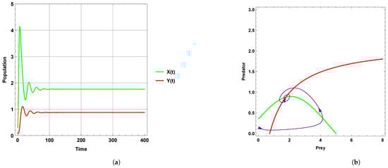
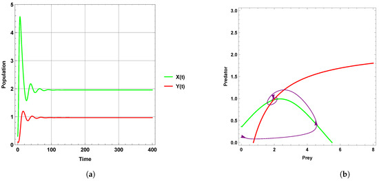
Figure 2.
Predator–prey dynamics of system (5) with the term when the value of : (a) time series; (b) zero isoclines and phase portrait trajectories.
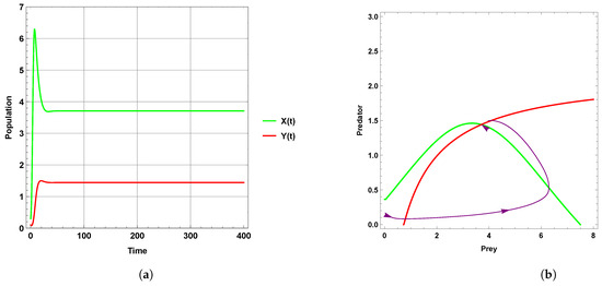
Figure 3.
Predator–prey dynamics of system (5) with the term when the value of : (a) time series; (b) zero isoclines and phase portrait trajectories.
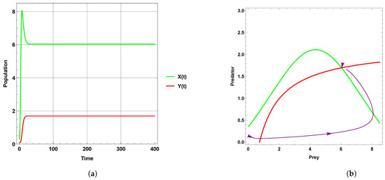
Figure 4.
Predator–prey dynamics of system (5) with the term when the value of : (a) time series; (b) zero isoclines and phase portrait trajectories.
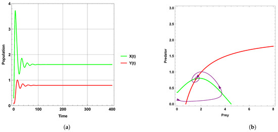
Figure 5.
Predator–prey dynamics of system (6) with the term when the value of : (a) time series; (b) zero isoclines and phase portrait trajectories.
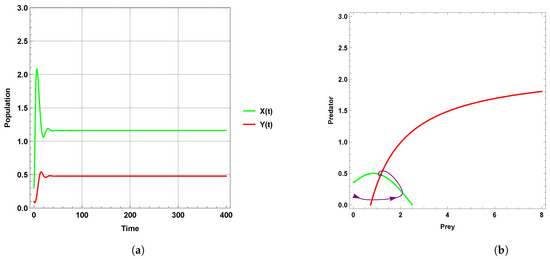
Figure 6.
Predator–prey dynamics of system (6) with the term when the value of : (a) time series; (b) zero isoclines and phase portrait trajectories.
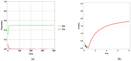
Figure 7.
Predator–prey dynamics of system (6) with the term when the value of : (a) time series; (b) zero isoclines and phase portrait trajectories.
4. Numerical Simulations of Periodic Perturbations
In this study, many numerical simulations of model (4) were executed to show the dynamic behaviors of predator–prey models with periodic seasonal perturbations of carrying capacity. Two patterns of dynamic behavior are observed in the classical ecological models of two interacting species: approaching the limit cycle or exhibiting stable dynamics. However, ecological communities in nature have been observed to display extremely complex dynamic behaviors. With the use of Mathematica software, the numerical simulations were executed based on parameter values that were selected so that non-autonomous system (4) is consistent with the theoretical assumptions in Section 3. These values take into account the persistence (i.e., Theorem 10) of prey and predators and the existence of both stable (i.e., Theorem 7) and limit cycle (i.e., Theorem 8) dynamics.
The initial conditions were selected for all numerical simulations as follows:
The first set of parameters were taken as the same values of parameter set (39), including the value of , which does not exist in models (5) and (6). The first set of parameters verifies the system’s stability and the persistence of both species’ dynamic behaviors.
As a result of using the first set of parameters for system (4), one obtains the following results.
When the periodic perturbations are taken into consideration, it is observed that there is a change in dynamics to become a limit cycle; different values of seasonality strength are assumed, and the dynamics remain a limit cycle, but when increasing the values, the size of the limit cycle increases, as shown in Figure 8, Figure 9 and Figure 10. A bifurcation diagram is a map that predicts the type of dynamical behavior (the system is in a periodic or equilibrium state) for a given parameter space. The bifurcation diagram presented in Figure 11 shows that the existence of a limit cycle is associated with the strength of seasonality. An additional bifurcation diagram is shown in Figure 12, which shows a Hopf bifurcation at carrying capacity K of system (4) when is selected as 0.5; system (4) shows the existence of a limit cycle. Furthermore, bifurcation diagrams present the local extreme density of species of prey and predator with respect to the strength of seasonality and carrying capacity, which shows that there is a clear increase in species densities as the values of seasonality strength and carrying capacity increase, as shown in Figure 11 and Figure 12, respectively, but the occurrence of periodic dynamics is dependent on the strength of seasonality.
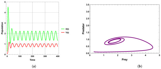
Figure 8.
Predator–prey dynamics of system (4) when : (a) time series; (b) phase portrait trajectories.
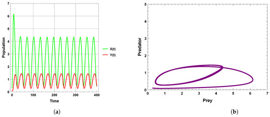
Figure 9.
Predator–prey dynamics of system (4) when : (a) time series; (b) phase portrait trajectories.
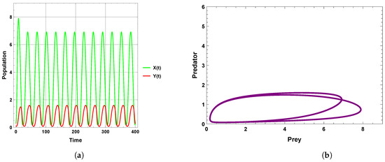
Figure 10.
Predator–prey dynamics of system (4) when : (a) time series; (b) phase portrait trajectories.
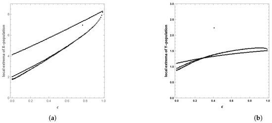
Figure 11.
Diagram of Hopf bifurcation with respect to seasonality strength of predator–prey dynamics of system (4) when : (a) time series; (b) phase portrait trajectories.
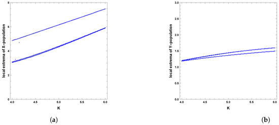
Figure 12.
Diagram of Hopf bifurcation with respect to carrying capacity K of predator–prey dynamics of system (4) with the second set of parameters and : (a) prey population and (b) predator population.
In system (4), the second set of parameters is supposed to be as follows:
A limit cycle is shown in Figure 13 with free seasonality effects that is considered a representation of the second of the main dynamics of non-autonomous model (4). It is concluded that the dynamics become more complex when periodic perturbations are present with increasing values of seasonality strength. In Figure 14, the dynamic is a quasi-limit cycle (periodic doubling) with more cycles, but the dynamics become chaotic, as shown in Figure 15 and Figure 16. It is observed that the bifurcation diagram presented in Figure 17 shows the existence of limit cycle doubling and chaos dynamics with seasonality strength. Through another bifurcation diagram, Figure 18 shows a Hopf bifurcation with respect to carrying capacity K of system (4), where was chosen as 0.5; system (4) displays the existence of limit cycle doubling and chaos dynamics. In the second set, it is observed that there is a slight increase in the densities of species with increasing values of strength of seasonality and carrying capacity, as presented in Figure 17 and Figure 18, respectively. This may be interpreted as the dynamics in this set being periodic, but the oscillations increasingly lead to chaos.
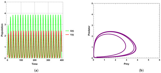
Figure 13.
Predator–prey dynamics of system (4) when : (a) time series; (b) phase portrait trajectories.
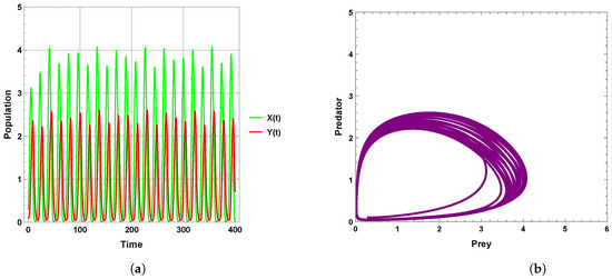
Figure 14.
Predator–prey dynamics of system (4) when : (a) time series; (b) phase portrait trajectories.
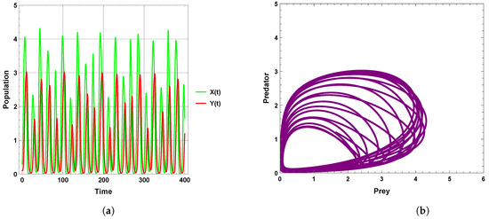
Figure 15.
Predator–prey dynamics of system (4) when : (a) time series; (b) phase portrait trajectories.
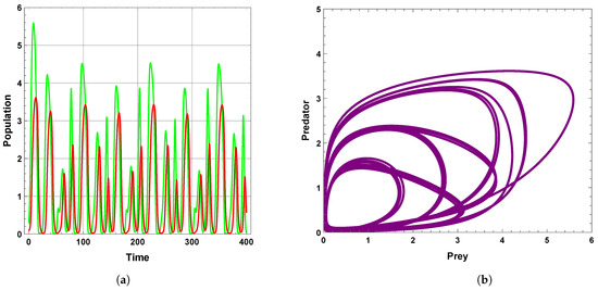
Figure 16.
Predator–prey dynamics of system (4) when : (a) time series; (b) phase portrait trajectories.
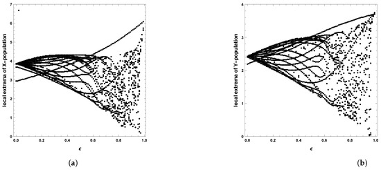
Figure 17.
Diagram of Hopf bifurcation with respect to seasonality strength of predator–prey dynamics of system (4) with the second set of parameters: (a) prey population and (b) predator population.
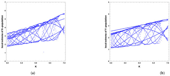
Figure 18.
Diagram of Hopf bifurcation with respect to carrying capacity K of predator–prey dynamics of system (4) with the second set of parameters and : (a) prey population and (b) predator population.
The obtained dynamics in the numerical simulations illustrate that periodic perturbations have a significant role in concluding more forms of dynamics, so rich dynamics are presented that make the model more realistic, especially in the second set of parameters. This may be explained from an ecological point of view by the fact that there are factors such as climate change, epidemics, and other causes that affect the dynamics of prey and predator systems. Volatility in dynamics makes these systems more vulnerable to extinction. The key results for different values of strength seasonality are summarized in Table 2, which involves the impact of sudden vs. periodic perturbations.
Table 2.
Summarizing the key results for different values of strength seasonality that involve the impact of sudden vs. periodic perturbations.
5. Concluding Remarks
The interaction between predators and prey is an important topic in mathematical ecology. In this paper, we present a novel predator–prey model by assuming a change in the carrying capacity with the Crowley–Martin functional response, which is considered one of the most general functional responses. Carrying capacity changes occur in two ways: sudden perturbations and periodic perturbations. We derived periodic perturbations by incorporating the sinusoidal function with the carrying capacity parameter, while we derive sudden perturbations by considering the sinusoidal function in specific cases, which represents the minimum and maximum values of the seasonality strength.
Systems (5) and (6), which represent predator–prey interactions with sudden perturbations, were analyzed mathematically through verifying their existence and positivity; proving the boundedness of the solution; obtaining the equlibria; studying the stability for each equilibrium point; obtaining their stability conditions; determining the Hopf bifurcation with respect to the carrying capacity; and finding the uniform persistence conditions of the model. The degree of seasonality and classification of circumstances plays a significant role in the uniqueness of the coexistence equilibrium point, the stability of the system, and the existence of a limit cycle. Furthermore, numerical simulations were used to demonstrate and validate our theoretical findings. The influence of periodic perturbations (i.e., system (4)) is computationally demonstrated, which shows the presence of different dynamics for prey and predator, such as the doubling of limit cycles and chaos dynamics, so this influence can diversify the range of possible solutions, which gives more realistic dynamics to interpret many of the changes that may exist in these systems from an ecological point of view. It would be interesting as future work to investigate more scenarios about the extinction of species under bad conditions, as it is inevitable for all parameter combinations.
The differences and connections between the obtained results in this study and results from previously conducted studies are as follows:
- The difference in the mechanism of describing the changes in the carrying capacity, which includes sudden and periodic perturbations represented as autonomous and non-autonomous models, respectively.
- Theoretical analysis demonstrates that the degree of seasonality and circumstances, whether good or bad, play an important role in the uniqueness of the coexistence equilibrium point, the stability of the system, the existence of a limit cycle, and the persistence, as shown through Theorems 3, 7, 8, and 10, respectively.
- To verify and explain the theoretical results, numerical simulations were also executed, showing that species densities increase with seasonality strength under good circumstances. However, species densities decrease as seasonality strength increases in the case of bad circumstances. Furthermore, predator species will become extinct if the seasonally strength value increases sufficiently in the case of bad circumstances.
- The numerical simulations show that there are rich and highly complex dynamics with periodic perturbations. This diversity of dynamics may explain many ecological phenomena.
- The numerical simulations show consistency with the literature on the effect of periodic disturbances on predator–prey models, which leads to a state of destabilization [31,32,33,34].
Funding
This research was funded by the Deanship of Postgraduate Studies and Scientific Research at Majmaah University through the project number (R-2025-1503).
Data Availability Statement
Data are contained within the article.
Acknowledgments
The author extends the appreciation to the Deanship of Postgraduate Studies and Scientific Research at Majmaah University for funding this research work through the project number (R-2025-1503).
Conflicts of Interest
The author declares no conflicts of interest.
References
- Lotka, A.J. Elements of Physical Biology; Williams & Wilkins: Columbia, MD, USA, 1925. [Google Scholar]
- Volterra, V. Variazioni e fluttuazioni del numero d’individui in specie animali conviventi. In Memoire Della Real Accademia Nazionale dei Lincei II; Accademia Nazionale dei Lincei: Rome, Italy, 1926; pp. 31–113. [Google Scholar]
- Kuang, Y. Basic properties of mathematical population models. J. Biomath 2002, 17, 129–142. [Google Scholar]
- Rockwood, L.L. Introduction to Population Ecology; Cambridge University Press: Cambridge, UK, 2006. [Google Scholar]
- Pastor, J. Mathematical Ecology of Populations and Ecosystems; Wiley-Blackwell: Hoboken, NJ, USA, 2008. [Google Scholar]
- Ajraldi, V.; Pittavino, M.; Venturino, E. Modeling herd behavior in population systems. Nonlinear Anal. Real World Appl. 2011, 12, 2319–2338. [Google Scholar] [CrossRef]
- Braza, P.A. Predator–prey dynamics with square root functional responses. Nonlinear Anal. Real World Appl. 2012, 13, 1837–1843. [Google Scholar] [CrossRef]
- Wang, X.; Zanette, L.; Zou, X. Modelling the fear effect in predator-prey interactions. J. Math. Biol. 2016, 73, 1179–1204. [Google Scholar] [CrossRef]
- Xie, B. Impact of the fear and Allee effect on a Holling type II prey–predator model. Adv. Differ. Equ. 2021, 2021, 464. [Google Scholar] [CrossRef]
- Alebraheem, J.; Abu-Hassan, Y. A novel mechanism measurement of predator interference in predator-prey models. J. Math. Biol. 2023, 86, 84. [Google Scholar] [CrossRef] [PubMed]
- Crowley, P.H.; Martin, E.K. Functional responses and interference within and between year classes of a dragonfly population. J. N. Am. Benth Soc. 1989, 8, 211–221. [Google Scholar] [CrossRef]
- Holling, C.S. Some characteristics of simple types of predation and parasitism. Can. Entomol. 1959, 91, 385–398. [Google Scholar] [CrossRef]
- Beddington, J.R. Mutual interference between parasites or predators and its effect on searching efficiency. J. Anim. Ecol. 1975, 51, 331–340. [Google Scholar] [CrossRef]
- DeAngelis, D.L.; Goldstein, R.A.; O’Neill, R.V. A model for trophic interaction. Ecology 1975, 56, 881–892. [Google Scholar] [CrossRef]
- Skalski, G.T.; Gilliam, J.F. Functional responses with predator interference: Viable alternatives to the Holling type II model. Ecology 2001, 82, 3083–3092. [Google Scholar] [CrossRef]
- Tripathi, J.P.; Abbas, S.; Thakur, M. Dynamical analysis of a prey–predator model with Beddington–DeAngelis type function response incorporating a prey refuge. Nonlinear Dyn. 2015, 80, 177–196. [Google Scholar] [CrossRef]
- Tripathi, J.P.; Abbas, S.; Thakur, M. A density dependent delayed predator–prey model with Beddington–DeAngelis type function response incorporating a prey refuge. Commun. Nonlinear Sci. Numer. Simul. 2015, 22, 427–450. [Google Scholar] [CrossRef]
- Parshad, R.D.; Basheer, A.; Jana, D.; Tripathi, J.P. Do prey handling predators really matter: Subtle effects of a Crowley–Martin functional response. Chaos Solitons Fractals 2017, 103, 410–421. [Google Scholar] [CrossRef]
- Upadhyay, R.K.; Naj, R.K. Dynamics of a three species food chain model with Crowley–Martin type functional response. Chaos Solit. Fractals 2009, 42, 1337–1346. [Google Scholar] [CrossRef]
- Alebraheem, J.; Abu-Hassan, Y. Simulation of complex dynamical behavior in prey predator model. In Proceedings of the 2012 International Conference on Statistics in Science, Business and Engineering (ICSSBE), Langkawi, Malaysia, 10–12 September 2012; IEEE: Piscataway, NJ, USA, 2012; pp. 1–4. [Google Scholar]
- Maiti, A.; Dubey, B.; Chakraborty, A. Global analysis of a delayed stage structure prey–predator model with Crowley–Martin type functional response. Math. Comput. Simul. 2019, 162, 58–84. [Google Scholar] [CrossRef]
- Mortoja Golam, S.K.; Panja, P.; Mondal, S.K. Dynamics of a predator–prey model with nonlinear incidence rate, Crowley–Martin type functional response and disease in prey population. Ecol. Gen. Genom. 2019, 10, 100035. [Google Scholar] [CrossRef]
- Xu, C.; Yu, Y.; Ren, G. Dynamic analysis of a stochastic predator–prey model with Crowley–Martin functional response, disease in predator, and saturation incidence. J. Comput. Nonlinear Dyn. 2020, 15, 071004. [Google Scholar] [CrossRef]
- Panja, P. Dynamics of a predator–prey model with Crowley–Martin functional response, refuge on predator and harvesting of super-predator. J. Biol. Syst. 2021, 29, 631–646. [Google Scholar] [CrossRef]
- Tripathi, J.P.; Bugalia, S.; Tiwari, V.; Kang, Y. A predator–prey model with Crowley–Martin functional response: A nonautonomous study. Nat. Resour. Model. 2020, 33, e12287. [Google Scholar] [CrossRef]
- Roy, S.S.; Tiwari, P.K.; Dubey, B. Dynamics of a stage-structured predator–prey system with fear-induced group defense in 368 autonomous and nonautonomous settings. Chaos 2024, 34, 063133. [Google Scholar] [CrossRef]
- Tiwari, V.; Tripathi, J.P.; Abbas, S.; Wang, J.S.; Sun, G.Q.; Jin, Z. Qualitative analysis of a diffusive Crowley–Martin predator–prey model: The role of nonlinear predator harvesting. Nonlinear Dyn. 2019, 98, 1169–1189. [Google Scholar] [CrossRef]
- Alebraheem, J. Dynamics of a Predator–Prey Model with the Effect of Oscillation of Immigration of the Prey. Diversity 2021, 13, 23. [Google Scholar] [CrossRef]
- Lu, C. Dynamical analysis and numerical simulations on a Crowley–Martin predator–prey model in stochastic environment. Appl. Math. Comput. 2022, 413, 126641. [Google Scholar] [CrossRef]
- Liang, Z.; Meng, X. Stability and Hopf bifurcation of a multiple delayed predator–prey system with fear effect, prey refuge and Crowley–Martin function. Chaos Solitons Fractals 2023, 175, 113955. [Google Scholar] [CrossRef]
- Gakkhar, S.; Naji, R.K. Seasonally perturbed prey–predator system with predator-dependent functional response. Chaos Solitons Fractals 2003, 18, 1075–1083. [Google Scholar] [CrossRef]
- Yu, H.; Zhao, M. Seasonally perturbed prey–predator ecological system with the Beddington–DeAngelis functional response. Discret. Dyn. Nat. Soc. 2012, 2012, 150359. [Google Scholar] [CrossRef]
- Alebraheem, J. Fluctuations in interactions of prey predator systems. Sci. Int. 2016, 28, 2357–2362. [Google Scholar]
- Sauve, A.M.; Taylor, R.A.; Barraqu, F. The effect of seasonal strength and abruptness on predator–prey dynamics. J. Theor. Biol. 2020, 491, 110175. [Google Scholar] [CrossRef] [PubMed]
- Alebraheem, J.; Elazab, N.S.; Mohammed, M.; Riahi, A.; Elmoasry, A. Deterministic sudden changes and stochastic fluctuation effects on stability and persistence dynamics of two-predator one-prey model. J. Math. 2021, 2021, 6611970. [Google Scholar] [CrossRef]
- Barman, D.; Upadhyay, R.K. Modelling Predator–Prey Interactions: A Trade-Off between Seasonality and Wind Speed. Mathematics 2023, 11, 4863. [Google Scholar] [CrossRef]
- Arif, G.E.; Alebraheem, J.; Yahia, W.B. Dynamics of Predator-prey Model under Fluctuation Rescue Effect. Baghdad Sci. J. 2023, 20, 1742. [Google Scholar] [CrossRef]
- Shepherd, J.J.; Stojikov, L. The logistic population model with slowly varying carrying capacity. Anziam J. 2007, 47, 492–506. [Google Scholar] [CrossRef]
- Al-Moqbali, M.K.; Al-Salti, N.S.; Elmojtaba, I.M. Prey–predator models with variable carrying capacity. Mathematics 2018, 6, 102. [Google Scholar] [CrossRef]
- Ang, T.K.; Safuan, H.M. Harvesting in a toxicated intraguild predator–prey fishery model with variable carrying capacity. Chaos Solitons Fractals 2019, 126, 158–168. [Google Scholar] [CrossRef]
- Al-Salti, N.; Al-Musalhi, F.; Gandhi, V.; Al-Moqbali, M.; Elmojtaba, I. Dynamical analysis of a prey–predator model incorporating a prey refuge with variable carrying capacity. Ecol. Complex. 2021, 45, 100888. [Google Scholar] [CrossRef]
- Schenzle, D. An age-structured model of pre-and post-vaccination measles transmission. Math. Med. Biol. J. IMA 1984, 1, 169–191. [Google Scholar] [CrossRef]
- Bolker, B.M. Chaos and complexity in measles models: A comparative numerical study. IMA J. Math. Appl. Med. Biol. 1993, 10, 83–95. [Google Scholar] [CrossRef]
- Earn, D.J.D.; Rohani, P.; Bolker, B.M.; Grenfell, B.T. A simple model for complex dynamical transitions in epidemics. Science 2000, 287, 667–670. [Google Scholar] [CrossRef] [PubMed]
- Keeling, M.J.; Rohani, P.; Grenfell, B.T. Seasonally forced disease dynamics explored as switching between attractors. Phys. D Nonlinear Phenom. 2001, 148, 317–335. [Google Scholar] [CrossRef]
- Freedman, H.I.; Ruan, S.G. Uniform persistence in functional differential equations. J. Differ. Equ. 1995, 115, 173–192. [Google Scholar] [CrossRef]
Disclaimer/Publisher’s Note: The statements, opinions and data contained in all publications are solely those of the individual author(s) and contributor(s) and not of MDPI and/or the editor(s). MDPI and/or the editor(s) disclaim responsibility for any injury to people or property resulting from any ideas, methods, instructions or products referred to in the content. |
© 2025 by the author. Licensee MDPI, Basel, Switzerland. This article is an open access article distributed under the terms and conditions of the Creative Commons Attribution (CC BY) license (https://creativecommons.org/licenses/by/4.0/).