Odd Exponential-Logarithmic Family of Distributions: Features and Modeling

Abstract

This paper introduces a general family of continuous distributions, based on the exponential-logarithmic distribution and the odd transformation. It is called the “odd exponential logarithmic family”. We intend to create novel distributions with desired qualities for practical applications, using the unique properties of the exponential-logarithmic distribution as an initial inspiration. Thus, we present some special members of this family that stand out for the versatile shape properties of their corresponding functions. Then, a comprehensive mathematical treatment of the family is provided, including some asymptotic properties, the determination of the quantile function, a useful sum expression of the probability density function, tractable series expressions for the moments, moment generating function, Rényi entropy and Shannon entropy, as well as results on order statistics and stochastic ordering. We estimate the model parameters quite efficiently by the method of maximum likelihood, with discussions on the observed information matrix and a complete simulation study. As a major interest, the odd exponential logarithmic models reveal how to successfully accommodate various kinds of data. This aspect is demonstrated by using three practical data sets, showing that an odd exponential logarithmic model outperforms two strong competitors in terms of data fitting.

1. Introduction

There has been a growing interest in defining new flexible distributions in the modern age, which has been submerged by the volume of data arriving from all disciplines. To define such mathematical objects, “thoroughly changing” a baseline (continuous) distribution is a straightforward and fast method. The addition of parameters has been shown to be useful in investigating tail properties as well as increasing the goodness-of-fit of the related models. Among the proposed distributions, the T-X family of continuous distributions (focds) by [1] is the most popular one. An exhaustive review of it can be found in [2]. Also, one of the most useful transformers for the T-X focds is the following odd transformation: $W\left[G\right(x;𝔍\left)\right]=G(x;𝔍)/[1-G(x;𝔍\left)\right]$, where $G(x;𝔍)$ denotes the cumulative density function (cdf) and 𝔍 the parameters of the cdf. That is, the focds defined by $G(x;𝔍)$ is modified, defining a new focd based on a transformed cdf through the use of $W\left[G\right(x;𝔍\left)\right]$. Such a transformed focds is generally called an “odd family” of distributions. Some odd families available in the modern literature are the odd log-logistic (OLL) focds by [3], odd-gamma generated type 3 (OGGT3) focds by [4], odd exponentiated generated (odd exp-G) focds by [5], odd Weibull generated (OW-G) focds by [6], odd generalized exponential (OGE) focds by [7], odd generalized exponential log-logistic (OGELL) focds by [8], odd log-logistic normal (OLLN) focds by [9], new generalized odd log-logistic (NGOLL) focds by [10], odd Fréchet generated (OF-G) focds by [11], generalized odd gamma generated (GOG-G) focds by [12], generalized odd Lindley generated (GOL-G) focds by [13], Marshall-Olkin odd Lindley generated (MOOL-G) focds by [14], extended odd generated (EO-G) focds by [15], generalized odd inverted exponential generated (GOIE-G) focds by [16], odd flexible Weibull-H (OFW-H) family by [17], transmuted odd Fréchet generated (TOF-G) focds by [18], odd generalized gamma generated (OGG-G) focds by [19], modified odd Weibull generated (MOW-G) focds by [20], Topp-Leone odd Fréchet generated (TLOF-G) focds by [21], weighted odd Weibull generated (WOW-G) focds by [22], additive odd (AO) focds by [23], exponentiated odd Chen-G (EOC-G) focds by [24], generalized odd linear exponential (GOLE) focds by [25], and sine extended odd Fréchet generated (SEOF-G) focds by [26].

The new idea in this paper is centered around the notorious exponential-logarithmic (EL) distribution introduced by [27]. The EL distribution plays a fundamental role in reliability in several disciplines such as manufacturing, finance, biological sciences, and engineering. It is mathematically defined as follows. Let $p\in (0,1)$ and $\beta >0$. Then, the EL distribution with parameters p and $\beta$ is defined by the following cdf:

$$\begin{array}{c}\hfill F_{*}(x;p,\beta )=1-\frac{1}{log\left(p\right)}log[1-(1-p)e^{-\beta x}],x>0.\end{array}$$

(1)

Thus, it has the feature of combining exponential and logarithmic functions.

The related probability density function (pdf) is given by

$$\begin{array}{c}\hfill f_{*}(x;p,\beta )=\left(\frac{1}{-log\left(p\right)}\right)\frac{\beta (1-p)e^{-\beta x}}{1-(1-p)e^{-\beta x}},x>0.\end{array}$$

This pdf has the following notable properties: it is strictly decreasing with respect to x, it tends to zero as $x\to +\infty$, it is unimodal with a modal value at $x=0$ and it is reduced to the pdf of the exponential distribution with rate parameter $\beta$ as $p\to 1$. Also, as a complementary key function, the corresponding hazard rate function (hrf) is given by

$$h_{*}(x;p,\beta )=\frac{-\beta (1-p)e^{-\beta x}}{[1-(1-p)e^{-\beta x}]log[1-(1-p)e^{-\beta x}]},x>0.$$

It is proved to be decreasing (contrary to the former exponential distribution having a constant hrf). As an advantage for statistical analysis, the quantile function (qf) of the EL distribution has a closed-form expression; it is given by

$$Q_{*}(u;p,\beta )=\frac{1}{\beta }log\left(\frac{1-p}{1-p^{1-u}}\right),u\in [0,1).$$

Also, the EL distribution has a solid physical interpretation. Indeed, consider $T={\left(T_n\right)}_{n\in {\mathbb{N}}^{*}}$ to be a sequence of independent and identically distributed random variables with an exponential distribution and a common parameter, $\beta$. Let N be a random variable following the discrete logarithmic distribution with parameter $1-p$, also independent of T. Then, the random variable $X=inf(T_1,\dots ,T_N)$ follows the EL distribution with parameters p and $\beta$. As an example, such a random variable can model the lifetime of a system that failed when one of its components failed, assuming that it is dependent on a random number of independent components represented by N and that the lifetime of the i-th component is represented by $T_i$.

We leverage these characteristics of the EL distribution to create a new odd focds based on it. We present three special four-parameter distributions of the family that have very desirable statistical properties, such as versatile hazard rate shapes; increasing, decreasing, J, reversed-J, and bathtub shapes. Then, a complete mathematical treatment of the focds is derived, with several results on the pdf, moments, entropy (Rényi and Shannon entropy), order statistics, and stochastic ordering. By turning out some special distributions as models, we prove that they are more adequate to fit some data sets than notable competitors, with the same or more numbers of parameters, and the same baseline distribution as well. We explain this success by the original exponential-logarithmic definitions of the corresponding functions, offering some ability in the modeling that can be reached by other families.

The paper is composed of the following sections. In Section 2, we introduce the odd exponential-logarithmic focds. We present some special distributions in Section 3. The mathematical properties of the focds are derived in Section 4. For the inferential aspect, the maximum likelihood method is discussed in Section 5. The analysis of two real data sets is presented to illustrate the modeling potential of the focds in Section 6. Finally, the conclusion of the paper appears in Section 7.

2. The New Family

The proposed focds, called the odd EL generated (OEL-G) focds, is characterized by the cdf given by

$$\begin{array}{c}\hfill F(x;p,\beta ,𝔍)=1-\frac{1}{log\left(p\right)}log\left[1-(1-p)e^{-\beta \frac{G(x;𝔍)}{1-G(x;𝔍)}}\right],x\in \mathbb{R},\end{array}$$

(2)

where $G(x;𝔍)$ denotes the cdf of an absolutely continuous distribution based on a parameter vector denoted by 𝔍. We recall that $p\in (0,1)$. Its definition is based on the T-X transformation introduced by [1], the EL distribution previously presented and the odd transformation, i.e., we can write $F(x;p,\beta ,𝔍)$ as $F(x;p,\beta ,𝔍)=F_{*}\left(W\left[G\right(x;𝔍\left)\right];p,\beta \right)$, where $F_{*}(y;p,\beta )$ is the cdf of the EL distribution given by (1) and $W\left(y\right)$ is the following odd transformation: $W\left(y\right)=y/(1-y)$. One can also notice some compounding relations between the OEL-G and the OW-G and Pappas and Loukas generated (PAL-G) families by [6,28], respectively. Indeed, we can write $F(x;p,\beta ,𝔍)$ as

$$\begin{array}{c}\hfill F(x;p,\beta ,𝔍)=1-\frac{1}{log\left(p\right)}log\left[1-(1-p)S_o(x;\beta ,𝔍)\right],\end{array}$$

where $S_o(x;\beta ,𝔍)$ denotes the survival function (sf) of the OW-G focds with parameters $\beta$ and 𝔍, which also corresponds to the cdf of the PAL-G focds, with parameter p and the cdf of the OW-G focds as a baseline. However, to the best of our knowledge, the OEL-G focds as defined by (2) is new in the literature.

The sf of the OEL-G focds is given by $S(x;p,\beta ,𝔍)=1-F(x;p,\beta ,𝔍)$, hence

$$\begin{array}{c}\hfill S(x;p,\beta ,𝔍)=\frac{1}{log\left(p\right)}log\left[1-(1-p)e^{-\beta \frac{G(x;𝔍)}{1-G(x;𝔍)}}\right],x\in \mathbb{R},\end{array}$$

The appropriate pdf is given by deriving $F(x;p,\beta ,𝔍)$ from x; we get

$$\begin{array}{c}\hfill f(x;p,\beta ,𝔍)=\left(\frac{1}{-log\left(p\right)}\right)\frac{g(x;𝔍)}{{[1-G(x;𝔍)]}^2}\frac{(1-p)\beta e^{-\beta \frac{G(x;𝔍)}{1-G(x;𝔍)}}}{1-(1-p)e^{-\beta \frac{G(x;𝔍)}{1-G(x;𝔍)}}},x\in \mathbb{R},\end{array}$$

(3)

where $g(x;𝔍)$ refers to the pdf related to $G(x;𝔍)$.

Also, the hrf of the OEL-G focds is specified by $h(x;p,\beta ,𝔍)=f(x;p,\beta ,𝔍)/S(x;p,\beta ,𝔍)$, hence

$$\begin{array}{cc}\hfill h(x;p,\beta ,𝔍)& =\frac{g(x;𝔍)}{{[1-G(x;𝔍)]}^2}\frac{-(1-p)\beta e^{-\beta \frac{G(x;𝔍)}{1-G(x;𝔍)}}}{\left[1-(1-p)e^{-\beta \frac{G(x;𝔍)}{1-G(x;𝔍)}}\right]log\left[1-(1-p)e^{-\beta \frac{G(x;𝔍)}{1-G(x;𝔍)}}\right]},x\in \mathbb{R}.\hfill \end{array}$$

These two last functions are crucial to handling some statistical features of the OEL-G focds, such as the possible adequateness of the related models to various kinds of data.

3. Special Distributions

Three special four-parameter distributions of the OEL-G focds are described in this section, all defined with well-established baseline distributions, namely: the Weibull, gamma, and Fréchet distributions.

3.1. The OELW Distribution

The OEL Weibull (OELW) distribution is now introduced. It is defined by the cdf given by (2) with the Weibull distribution as baseline distribution, i.e., with the cdf given by $G(x;a,b)=1-e^{-{(x/b)}^a}$ and the pdf given by $g(x;a,b)=(a/b){(x/b)}^{a-1}{e}^{-{(x/b)}^a}$, $a,b,x>0$. When $x\le 0$, the cdf and pdf are equal to 0. Thus, the cdf of the OELW distribution is given by

$$\begin{array}{c}\hfill F(x;p,\beta ,a,b)=1-\frac{1}{log\left(p\right)}log\left[1-(1-p)e^{-\beta \left\{e^{{\left(\frac{x}{b}\right)}^a}-1\right\}}\right],x>0.\end{array}$$

In this setting, the pdf is expressed as

$$\begin{array}{c}\hfill f(x;p,\beta ,a,b)=\left(\frac{1}{-log\left(p\right)}\right)\frac{a}{b}{\left(\frac{x}{b}\right)}^{a-1}{e}^{{\left(\frac{x}{b}\right)}^a}\frac{(1-p)\beta e^{-\beta \left\{e^{{\left(\frac{x}{b}\right)}^a}-1\right\}}}{1-(1-p)e^{-\beta \left\{e^{{\left(\frac{x}{b}\right)}^a}-1\right\}}},x>0.\end{array}$$

The hrf is obtained as

$$\begin{array}{cc}\hfill h(x;p,\beta ,a,b)& =\frac{a}{b}{\left(\frac{x}{b}\right)}^{a-1}{e}^{{\left(\frac{x}{b}\right)}^a}\frac{-(1-p)\beta e^{-\beta \left\{e^{{\left(\frac{x}{b}\right)}^a}-1\right\}}}{\left[1-(1-p)e^{-\beta \left\{e^{{\left(\frac{x}{b}\right)}^a}-1\right\}}\right]log\left[1-(1-p)e^{-\beta \left\{e^{{\left(\frac{x}{b}\right)}^a}-1\right\}}\right]},x>0.\hfill \end{array}$$

The functions above are equal to 0 when $x\le 0$. As graphical illustrations, Figure 1 shows some plots of $f(x;p,\beta ,a,b)$ and $h(x;p,\beta ,a,b)$, for selected values of the parameters p, $\beta$, a and b. These plots show that the pdf of the OELW distribution has a great shape flexibility. It can be left skewed, right skewed, J-shaped, reversed J-shape, and symmetric. Furthermore, the corresponding hrf can be increasing, decreasing, J, or bathtub in shape.

Figure 1. Examples of plots of the (a) pdf and (b) hrf of the OELW distribution for various values of p, $\beta$, a and b.

The applicability of the OLEW distribution will be highlighted in the application part of the paper (see Section 6).

3.2. Two Other Examples

To show other perspectives of lifetime modeling, two other special cases are briefly described below.

3.2.1. The OELGa Distribution

We now introduce the OEL gamma (OELGa) distribution. It is defined by the cdf given by (2) with the gamma distribution as baseline distribution, i.e., with the cdf given by $G(x;a,b)=(1/\mathsf{\Gamma }(a\left)\right)\gamma (a,bx)$ and the pdf given by $g(x;a,b)=(b^a/\mathsf{\Gamma }\left(a\right))x^{\alpha -1}{e}^{-bx}$, $a,b,x>0$, where $\mathsf{\Gamma }\left(a\right)={\int }_0^{+\infty }{t}^{a-1}{e}^{-t}dt$ and $\gamma (a,bx)={\int }_0^{bx}{t}^{a-1}{e}^{-t}dt$. When $x\le 0$, the cdf and pdf are equal to 0. So, the cdf of the OELGa distribution is given by

$$\begin{array}{c}\hfill F(x;p,\beta ,a,b)=1-\frac{1}{log\left(p\right)}log\left[1-(1-p)e^{-\beta \frac{\gamma (a,bx)}{\mathsf{\Gamma }\left(a\right)-\gamma (a,bx)}}\right],x>0.\end{array}$$

The related pdf is given as

$$\begin{array}{c}\hfill f(x;p,\beta ,a,b)=\left(\frac{1}{-log\left(p\right)}\right)b^a{x}^{\alpha -1}{e}^{-bx}\frac{\gamma (a,bx)}{{[\mathsf{\Gamma }\left(a\right)-\gamma (a,bx)]}^2}\frac{(1-p)\beta e^{-\beta \frac{\gamma (a,bx)}{\mathsf{\Gamma }\left(a\right)-\gamma (a,bx)}}}{1-(1-p)e^{-\beta \frac{\gamma (a,bx)}{\mathsf{\Gamma }\left(a\right)-\gamma (a,bx)}}},x>0.\end{array}$$

The hrf is given by

$$\begin{array}{cc}\hfill h(x;p,\beta ,a,b)& =b^a{x}^{\alpha -1}{e}^{-bx}\frac{\gamma (a,bx)}{{[\mathsf{\Gamma }\left(a\right)-\gamma (a,bx)]}^2}\times \hfill \\ \hfill & \frac{-(1-p)\beta e^{-\beta \frac{\gamma (a,bx)}{\mathsf{\Gamma }\left(a\right)-\gamma (a,bx)}}}{\left[1-(1-p)e^{-\beta \frac{\gamma (a,bx)}{\mathsf{\Gamma }\left(a\right)-\gamma (a,bx)}}\right]log\left[1-(1-p)e^{-\beta \frac{\gamma (a,bx)}{\mathsf{\Gamma }\left(a\right)-\gamma (a,bx)}}\right]},x>0.\hfill \end{array}$$

The functions above are equal to 0 when $x\le 0$. Figure 2 shows some plots of $f(x;p,\beta ,a,b)$ and $h(x;p,\beta ,a,b)$, for selected values of the parameters p, $\beta$, a and b. The plots indicate that the pdf of the OELGa distribution can be reverse J-shaped, symmetric, right skewed, left-skewed, and unimodal, whereas the hrf of the OELGa has J and increasing shapes.

Figure 2. Examples of plots of the (a) pdf and (b) hrf of the OELGa distribution for various values of p, $\beta$, a and b.

3.2.2. The OELF Distribution

We now introduce the OEL Fréchet (OELF) distribution. It is defined by the cdf given by (2) with the Fréchet distribution as baseline distribution, i.e., with the cdf given by $G(x;a,b)=e^{-{(x/b)}^{-a}}$ and the pdf given by $g(x;a,b)=(a/b){(x/b)}^{-a-1}{e}^{-{(x/b)}^{-a}}$, $a,b,x>0$. When $x\le 0$, the cdf and pdf are equal to 0. Hence, the cdf of the OELF distribution is given by

$$\begin{array}{c}\hfill F(x;p,\beta ,a,b)=1-\frac{1}{log\left(p\right)}log\left[1-(1-p)e^{-\beta \frac{e^{-{\left(\frac{x}{b}\right)}^{-a}}}{1-e^{-{\left(\frac{x}{b}\right)}^{-a}}}}\right],x>0.\end{array}$$

The pdf can be deduced as

$$\begin{array}{c}\hfill f(x;p,\beta ,a,b)=\left(\frac{1}{-log\left(p\right)}\right)\frac{a}{b}{\left(\frac{x}{b}\right)}^{-a-1}\frac{e^{-{\left(\frac{x}{b}\right)}^{-a}}}{{[1-e^{-{\left(\frac{x}{b}\right)}^{-a}}]}^2}\frac{(1-p)\beta e^{-\beta \frac{e^{-{\left(\frac{x}{b}\right)}^{-a}}}{1-e^{-{\left(\frac{x}{b}\right)}^{-a}}}}}{1-(1-p)e^{-\beta \frac{e^{-{\left(\frac{x}{b}\right)}^{-a}}}{1-e^{-{\left(\frac{x}{b}\right)}^{-a}}}}},x>0.\end{array}$$

The hrf is expressed as

$$\begin{array}{cc}\hfill h(x;p,\beta ,a,b)& =\frac{a}{b}{\left(\frac{x}{b}\right)}^{-a-1}\frac{e^{-{\left(\frac{x}{b}\right)}^{-a}}}{{[1-e^{-{\left(\frac{x}{b}\right)}^{-a}}]}^2}\times \hfill \\ \hfill & \frac{-(1-p)\beta e^{-\beta \frac{e^{-{\left(\frac{x}{b}\right)}^{-a}}}{1-e^{-{\left(\frac{x}{b}\right)}^{-a}}}}}{\left[1-(1-p)e^{-\beta \frac{e^{-{\left(\frac{x}{b}\right)}^{-a}}}{1-e^{-{\left(\frac{x}{b}\right)}^{-a}}}}\right]log\left[1-(1-p)e^{-\beta \frac{e^{-{\left(\frac{x}{b}\right)}^{-a}}}{1-e^{-{\left(\frac{x}{b}\right)}^{-a}}}}\right]},x>0.\hfill \end{array}$$

The functions above are equal to 0 when $x\le 0$. Figure 3 shows some plots of $f(x;p,\beta ,a,b)$ and $h(x;p,\beta ,a,b)$, for selected values of the parameters p, $\beta$, a and b. The plots indicate that the OELF distribution can be reverse J-shaped, right skewed, left-skewed, and unimodal. On the other hand, the corresponding hrf has decreasing, increasing, J, reverse J- shapes.

Figure 3. Examples of plots of the (a) pdf and (b) hrf of the OELF distribution for various values of p, $\beta$, a and b.

4. Mathematical Features

This section is devoted to some mathematical properties of the OEL-G focds. In the following, it is assumed that the criterion for interchanging summation and integration and the criterion for interchanging summation and differentiation are satisfied. Also, let us mention that most of the presented formulas can be handled in standard mathematical software (Mathematica, Maple, …).

4.1. Asymptotic Results

Here, we investigate some asymptotic results of the pdf and hrf of the OEL-G focds.

First of all, as $x\to -\infty$ (or $G(x;𝔍)\to 0$), we have

$$f(x;p,\beta ,𝔍)\sim \left(\frac{1-p}{-plog\left(p\right)}\right)\beta g(x;𝔍),h(x;p,\beta ,𝔍)\sim \left(\frac{1-p}{-plog\left(p\right)}\right)\beta g(x;𝔍).$$

When $x\to +\infty$ (or $G(x;𝔍)\to 1$), we have

$$f(x;p,\beta ,𝔍)\sim \left(\frac{1-p}{-log\left(p\right)}\right)\beta \frac{g(x;𝔍)}{{[1-G(x;𝔍)]}^2}{e}^{-\beta \frac{G(x;𝔍)}{1-G(x;𝔍)}},h(x;p,\beta ,𝔍)\sim \beta \frac{g(x;𝔍)}{{[1-G(x;𝔍)]}^2}.$$

We thus see the role of the parameters $\beta$ and p in the possible asymptotes for these functions. In particular, when $x\to +\infty$, we see that $\beta$ has large impact on the convergence of $f(x;p,\beta ,𝔍)$ due to the exponential term, whereas p has no effect on the limit of $h(x;p,\beta ,𝔍)$. Also, the function $u\left(p\right)=(1-p)/[-plog(p\left)\right]$ appearing multiple times is decreasing in p and convex, with ${lim}_{p\to 0}u\left(p\right)=+\infty$ and ${lim}_{p\to 1}u\left(p\right)=0$.

4.2. Shapes of the pdf and hrf

The shapes of the pdf and hrf of the OEL-G focds can be described analytically. The critical point(s) of the pdf (also called mode(s)) of the OEL-G focds is(are) the root(s) of the following equation: $d\left[log\left(f\right(x;p,\beta ,𝔍\left)\right)\right]/dx=0$, i.e.,

$$\frac{dg(x;𝔍)/dx}{g(x;𝔍)}+2\frac{g(x;𝔍)}{1-G(x;𝔍)}-\beta \frac{g(x;𝔍)}{{[1-G(x;𝔍)]}^2}\frac{1}{\left[1-(1-p)e^{-\beta \frac{G(x;𝔍)}{1-G(x;𝔍)}}\right]}=0.$$

Similarly, the critical point(s) of the hrf of the OEL-G focds is(are) the root(s) of the following equation: $d\left[log\left(h\right(x;p,\beta ,𝔍\left)\right)\right]/dx=0$, i.e.,

$$\begin{array}{cc}\hfill & \frac{dg(x;𝔍)/dx}{g(x;𝔍)}+2\frac{g(x;𝔍)}{1-G(x;𝔍)}-\beta \frac{g(x;𝔍)}{{[1-G(x;𝔍)]}^2}\frac{1}{\left[1-(1-p)e^{-\beta \frac{G(x;𝔍)}{1-G(x;𝔍)}}\right]}\times \hfill \\ \hfill & \left(1+(1-p)\frac{e^{-\beta \frac{G(x;𝔍)}{1-G(x;𝔍)}}}{log\left[1-(1-p)e^{-\beta \frac{G(x;𝔍)}{1-G(x;𝔍)}}\right]}\right)=0.\hfill \end{array}$$

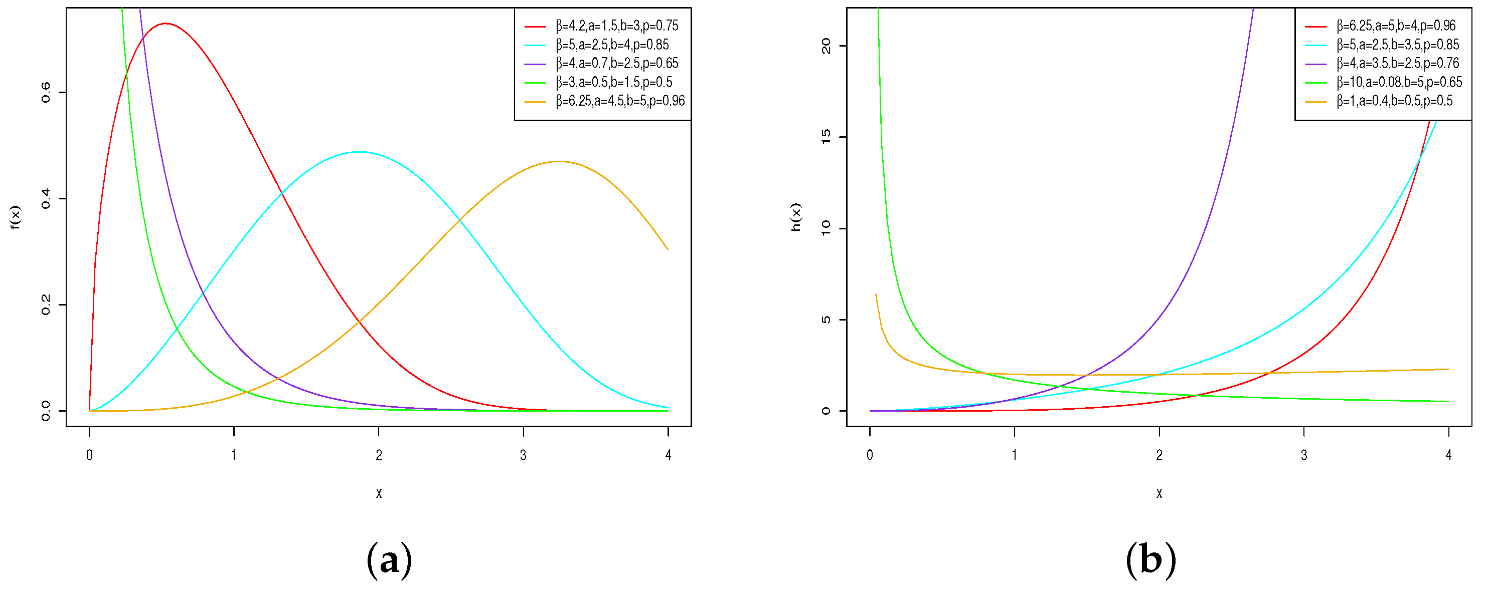
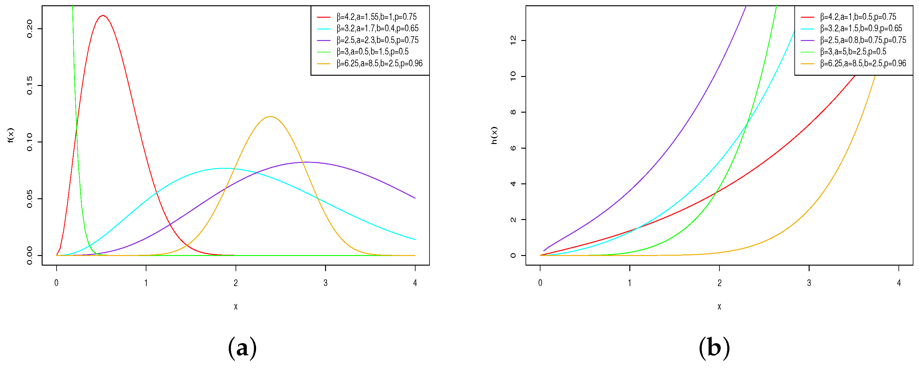
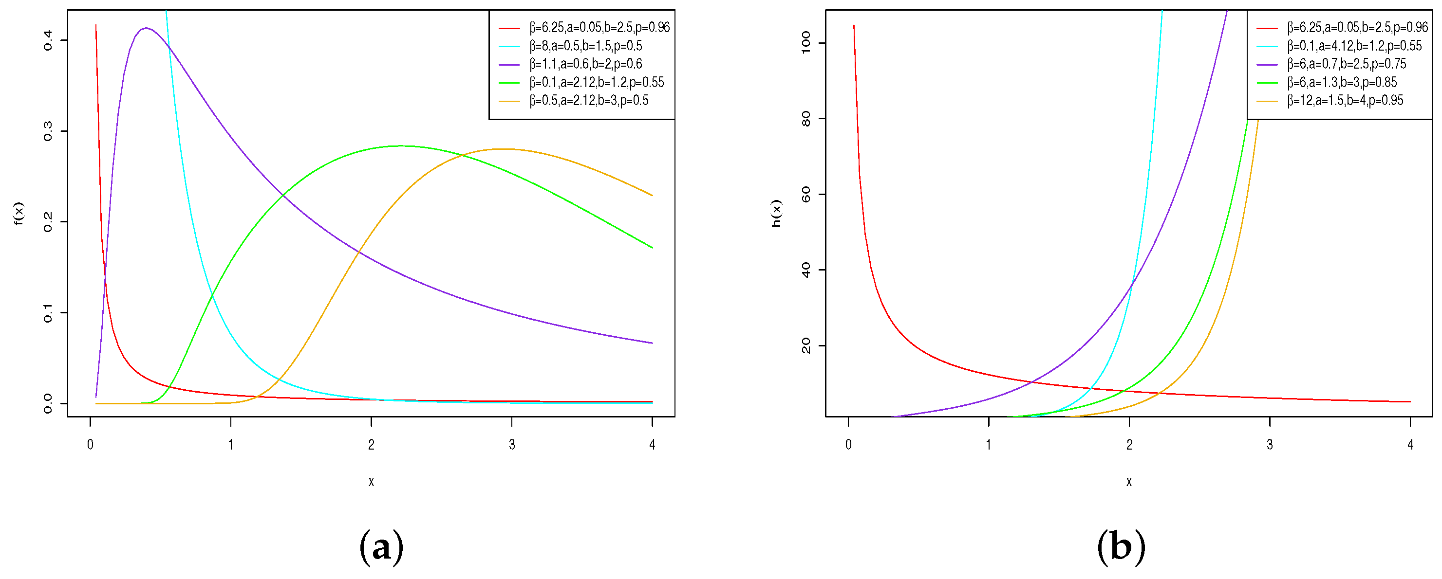
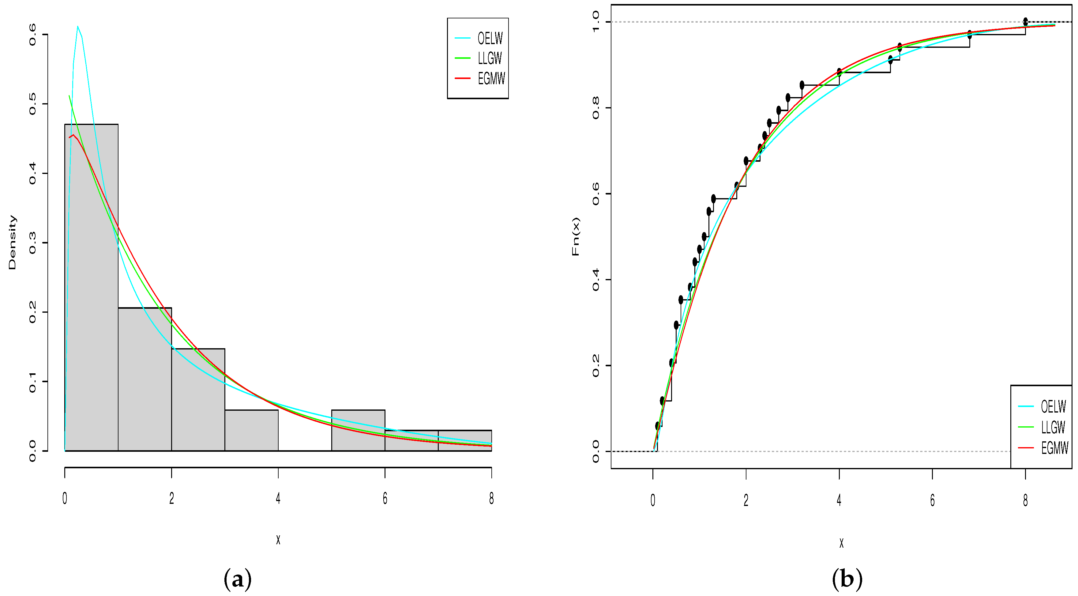
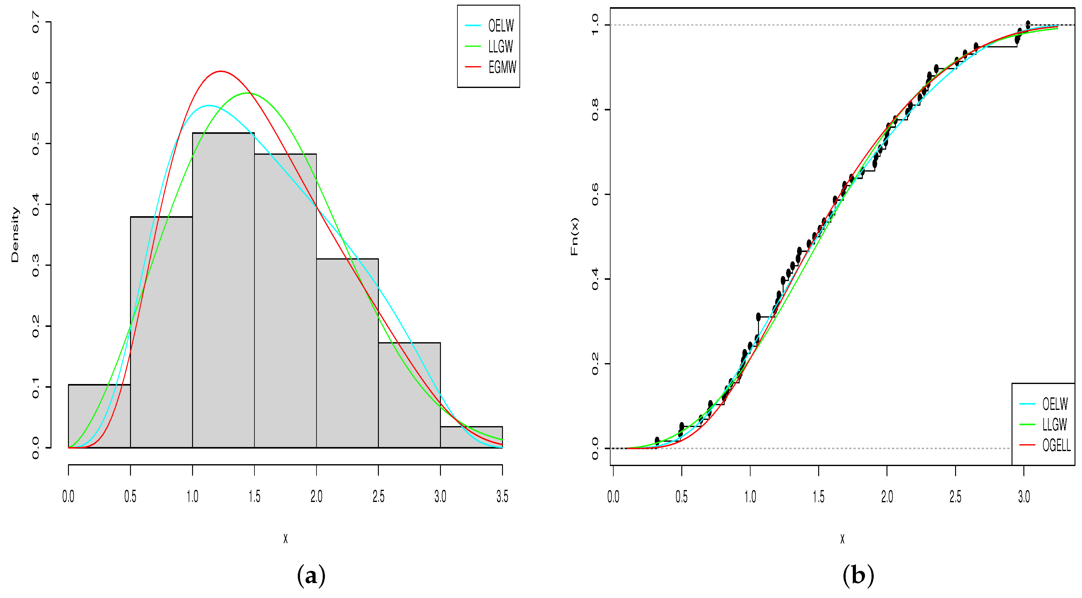
Mathematical software (R, Python, Mathematica, …) can be used to solve these two equations and determine whether the critical points are local maximums, minimums, or inflexion points for a given cdf $G(x;𝔍)$. It is the case for the proposed OELW, OELGa, and OELF distributions, where the equations above have no analytical solutions. For them, Figure 1, Figure 2 and Figure 3, are informative on their global mode properties; these special distributions can be unimodal, with various hrf shapes.

4.3. Quantile Function

The qf of the OEL-G focds, say $Q(u;p,\beta ,𝔍)$, satisfies the following functional equation:

$F\left(Q\right(u;p,\beta ,𝔍);p,\beta ,𝔍))=Q(F(u;p,\beta ,𝔍);p,\beta ,𝔍\left)\right)=u$, $u\in (0,1)$. After some algebraic manipulations, we get

$$\begin{array}{c}\hfill Q(u;p,\beta ,𝔍)=Q_G\left(\frac{log\left(\frac{1-p}{1-p^{1-u}}\right)}{\beta +log\left(\frac{1-p}{1-p^{1-u}}\right)};𝔍\right)u\in (0,1),\end{array}$$

(4)

where $Q_G(u;𝔍)$ denotes the qf related to $G(x;𝔍)$. As a result, with appropriate values of u, quantiles of interest can be obtained. In particular, the median is reduced to

$$M=Q(0.5;p,\beta ,𝔍)=Q_G\left(\frac{log\left(1+\sqrt{p}\right)}{\beta +log\left(1+\sqrt{p}\right)};𝔍\right).$$

One can also use the quantile function for simulating values for a special OEL-G distribution. For any random variable U with the standard uniform distribution, $X=Q(U;p,\beta ,𝔍)$ has the cdf given by (2).

4.4. Expansions of the cdf and pdf

The cdf and pdf of the OEL-G focds are expressed here using exp-G cdfs and pdfs as defined by [29]. Then, the structural properties of the exp-G focds can be used to derive those of the OEL-G focds.

The following result is about the series expansion of the cdf.

Proposition 1.

Let $F(x;p,\beta ,𝔍)$ be the cdf given by (2). Then, assuming that $G(x;𝔍)\in (0,1)$, the following series expansion is valid:

$$\begin{array}{c}\hfill F(x;p,\beta ,𝔍)=\sum _{k,\ell =1}^{+\infty }\sum _{m=0}^{+\infty }{a}_{k,\ell ,m}G{(x;𝔍)}^{\ell +m},\end{array}$$

where

$$\begin{array}{c}\hfill a_{k,\ell ,m}=\frac{1}{log\left(p\right)}{(-1)}^{\ell +m}\left(\genfrac{}{}{0pt}{}{-\ell }{m}\right)\frac{1}{k}\frac{1}{\ell !}{(1-p)}^k{\beta }^{\ell }{k}^{\ell }.\end{array}$$

(5)

Proof. 

It follows from the Taylor theorem applied to the logarithmic function that $log(1-x)=-{\displaystyle \sum _{k=1}^{+\infty }}\frac{1}{k}{x}^k$, $x\in (-1,1)$, and some sum manipulations, that

$$\begin{array}{cc}\hfill F(x;p,\beta ,𝔍)& =1+\frac{1}{log\left(p\right)}\sum _{k=1}^{+\infty }\frac{1}{k}{(1-p)}^k{e}^{-\beta k\frac{G(x;𝔍)}{1-G(x;𝔍)}}\hfill \\ \hfill & =\frac{1}{log\left(p\right)}\sum _{k=1}^{+\infty }\frac{1}{k}{(1-p)}^k\left[e^{-\beta k\frac{G(x;𝔍)}{1-G(x;𝔍)}}-1\right].\hfill \end{array}$$

For the term in brackets, the Taylor theorem applied to the exponential function, i.e., $e^x={\displaystyle \sum _{k=0}^{+\infty }}\frac{1}{k!}{x}^k$, $x\in \mathbb{R}$, gives

$$\begin{array}{c}\hfill e^{-\beta k\frac{G(x;𝔍)}{1-G(x;𝔍)}}-1=\sum _{\ell =1}^{+\infty }\frac{1}{\ell !}{(-1)}^{\ell }{\beta }^{\ell }{k}^{\ell }G{(x;𝔍)}^{\ell }{[1-G(x;𝔍)]}^{-\ell }.\end{array}$$

Now, the generalized binomial theorem, i.e., ${(1-x)}^{\upsilon }={\displaystyle \sum _{k=0}^{+\infty }}\left(\genfrac{}{}{0pt}{}{\upsilon }{k}\right){(-1)}^k{x}^k$, $x\in (-1,1)$, $\upsilon \in \mathbb{R}$, gives

$$\begin{array}{c}\hfill {[1-G(x;𝔍)]}^{-\ell }=\sum _{m=0}^{+\infty }\left(\genfrac{}{}{0pt}{}{-\ell }{m}\right){(-1)}^{m}G{(x;𝔍)}^m.\end{array}$$

By combining all of the foregoing equalities, we get the desired result. The proof of Proposition 1 is now complete. □

Corollary 1.

Owing to Proposition 1, upon differentiation of the involved functions, a series expansion for $f(x;p,\beta ,𝔍)$ is given by

$$\begin{array}{c}\hfill f(x;p,\beta ,𝔍)=\sum _{k,\ell =1}^{+\infty }\sum _{m=0}^{+\infty }{b}_{k,\ell ,m}g(x;𝔍)G{(x;𝔍)}^{\ell +m-1},\end{array}$$

where $b_{k,\ell ,m}=(\ell +m)a_{k,\ell ,m}$.

In comparison to the former analytical definition, for practical purposes (integration…), the expression of $f(x;p,\beta ,𝔍)$ in Corollary 1 can be more easy to handle through the following approximation:

$$\begin{array}{c}\hfill f(x;p,\beta ,𝔍)\approx \sum _{k,\ell =1}^M\sum _{m=0}^M{b}_{k,\ell ,m}g(x;𝔍)G{(x;𝔍)}^{\ell +m-1},\end{array}$$

where M is a carefully chosen number.

4.5. Moments

Hereafter, we denote by X a random variable having the cdf of the OEL-G focds given by (2). Corollary 1 can be used to have a tractable expression for the moments of X, among other things. Indeed, for any integer r, the rth moment of X is given by

$${\mu }_r^{\prime }=E\left(X^r\right)={\int }_{-\infty }^{+\infty }{x}^{r}f(x;p,\beta ,𝔍)dx=\sum _{k,\ell =1}^{+\infty }\sum _{m=0}^{+\infty }{b}_{k,\ell ,m}{\tau }_{\ell ,m,r},$$

where ${\tau }_{\ell ,m,r}={\int }_{-\infty }^{+\infty }{x}^{r}g(x;𝔍)G{(x;𝔍)}^{\ell +m-1}dx={\int }_0^1{u}^{\ell +m-1}{\left[Q_G(u;𝔍)\right]}^{r}du$. For a given $G(x;𝔍)$, this integral can be calculated or computed numerically. We refer to [30], where ${\tau }_{\ell ,m,r}$ has been determined for some standard distributions (normal, beta, Weibull …). For practical purposes, another remark concerns the infinity limit in the sums; as mentioned before, it can be substituted by a large positive integer.

As usual, the mean of X is obtained directly by $\mu ={\mu }_1^{\prime }$. Also, the variance of X can be calculated using the following formula: ${\sigma }^2={\mu }_2^{\prime }-{\mu }^2$.

In a similar vein, for $y\in \mathbb{R}$, the rth incomplete moment of X is given by

$${\mu }_r^{\prime }\left(y\right)=E\left(X^r{1}_{\{X\le y\}}\right)={\int }_{-\infty }^y{x}^{r}f(x;p,\beta ,𝔍)dx=\sum _{k,\ell =1}^{+\infty }\sum _{m=0}^{+\infty }{b}_{k,\ell ,m}{\tau }_{\ell ,m,r}\left(y\right),$$

where ${\tau }_{\ell ,m,r}\left(y\right)={\int }_{-\infty }^y{x}^{r}g(x;𝔍)G{(x;𝔍)}^{\ell +m-1}dx={\int }_0^{G(y;𝔍)}{u}^{\ell +m-1}{\left[Q_G(u;𝔍)\right]}^{r}du$. Then, one can express the mean deviations about the mean and about the median, as well as Bonferroni and Lorenz curves, which play a central role in life testing, reliability, and renewal theory.

Similarly, the moment generating function of X is given by

$$M\left(t\right)=E\left(e^{tX}\right)={\int }_{-\infty }^{+\infty }{e}^{tx}f(x;p,\beta ,𝔍)dx=\sum _{k,\ell =1}^{+\infty }\sum _{m=0}^{+\infty }{b}_{k,\ell ,m}{\upsilon }_{\ell ,m}\left(t\right),$$

where ${\upsilon }_{\ell ,m}\left(t\right)={\int }_{-\infty }^{+\infty }{e}^{tx}g(x;𝔍)G{(x;𝔍)}^{\ell +m-1}dx={\int }_0^1{u}^{\ell +m-1}{e}^{t{Q}_G(u;𝔍)}du$.

4.6. Skewness and Kurtosis

The skewness and kurtosis properties of the OEL-G focds can be explored via the four first moments or the use of the qf given by (4). The main measures defined by moments are the skewness and kurtosis parameters defined by

$$S=E\left[{\left(\frac{X-\mu }{\sigma }\right)}^3\right]=\frac{{\mu }_3^{\prime }-3{\mu }_2^{\prime }\mu +2{\mu }^3}{{\sigma }^3}$$

and

$$K=E\left[{\left(\frac{X-\mu }{\sigma }\right)}^4\right]=\frac{{\mu }_4^{\prime }-4{\mu }_3^{\prime }\mu +6{\mu }_2^{\prime }{\mu }^2-3{\mu }^4}{{\sigma }^4}.$$

They can be expressed for a given baseline cdf $G(x;𝔍)$.

Alternatively, if the moments do not exist (or in full generality), one can consider the measures defined with the qf. Examples are the Bowley skewness and the Moors kurtosis defined by, respectively,

$$S_{*}=\frac{Q(\frac{1}{4};p,\beta ,𝔍)+Q(\frac{3}{4};p,\beta ,𝔍)-2Q(\frac{1}{2};p,\beta ,𝔍)}{Q(\frac{3}{4};p,\beta ,𝔍)-Q(\frac{1}{4};p,\beta ,𝔍)},$$

and

$$K_{*}=\frac{Q(\frac{7}{8};p,\beta ,𝔍)-Q(\frac{5}{8};p,\beta ,𝔍)+Q(\frac{3}{8};p,\beta ,𝔍)-Q(\frac{1}{8};p,\beta ,𝔍)}{Q(\frac{6}{8};p,\beta ,𝔍)-Q(\frac{2}{8};p,\beta ,𝔍)}.$$

We refer to [31,32] for more information on these quantile measures.

Table 1 provides the mean, variance, skewness S and kurtosis K (defined with the moments) of one of the members of the OEL-G focds, the OELW distribution, for different choices of parameter values.

Table 1. Moment measures of the OELW distribution for various choices of parameters.

Parameter	Mean	Variance	Skewness	Kurtosis
$a=0.5$	0.1375667	0.05076667	12.77926	21.5475
$b=1.5$
$\beta =3$
$p=0.5$
$a=0.5$	0.06894464	0.03067229	27.02119	42.1311
$b=1.5$
$\beta =3$
$p=0.05$
$a=0.5$	0.04940314	0.02260463	38.03328	57.77719
$b=1.5$
$\beta =3$
$p=0.012$
$a=0.5$	1.324836	6.267231	8.523013	13.13688
$b=2$
$\beta =0.3$
$p=0.2$
$a=0.5$	$7.938928\times {10}^{-8}$	$1.69951\times {10}^{-10}$	26,964.99	26,960.99
$b=0.02$
$\beta =30$
$p=0.012$
$a=0.5$	0.1737497	0.09645452	15.83522	27.64176
$b=5$
$\beta =6.25$
$p=0.96$

Table 1 indicates that, for fixed a, b and $\beta$, the mean and variance of the OELW distribution are decreasing functions with respect to p. Also, the OELW distribution tends to be skewed more to the right as p decreases.

4.7. Entropy

Entropy is a measure of the variation of uncertainty that finds numerous applications in various areas such as engineering, mathematical physics, and probability. One of the most famous useful entropy measures is the Rényi entropy, introduced by [33] and the Shannon entropy by [34]. In the context of the OEL-G focds, the Rényi entropy of X is defined by

$$I_{\delta }\left(X\right)=\frac{1}{1-\delta }log\left[{\int }_{-\infty }^{+\infty }f{(x;p,\beta ,𝔍)}^{\delta }dx\right],$$

where $\delta >0$ and $\delta \ne 1$. As an alternative to direct computation, we now present an expression that depends on a tractable series expansion. In this regard, let us present and prove the following proposition, which can be viewed as an extension of Corollary 1.

Proposition 2.

Let $\delta \in \mathbb{R}$ and $f(x;p,\beta ,𝔍)$ be the pdf given by (3). Then, the following series expansion is valid:

$$\begin{array}{c}\hfill f{(x;p,\beta ,𝔍)}^{\delta }=\sum _{k,\ell ,m=0}^{+\infty }{c}_{k,\ell ,m}\left(\delta \right)g{(x;𝔍)}^{\delta }G{(x;𝔍)}^{\ell +m},\end{array}$$

where

$$\begin{array}{c}\hfill c_{k,\ell ,m}\left(\delta \right)={\left(\frac{1}{-log\left(p\right)}\right)}^{\delta }\left(\genfrac{}{}{0pt}{}{-\delta }{k}\right)\left(\genfrac{}{}{0pt}{}{-(2\delta +\ell )}{m}\right){(-1)}^{k+\ell +m}\frac{1}{\ell !}{(1-p)}^{\delta +k}{\beta }^{\delta +\ell }{(\delta +k)}^{\ell }.\end{array}$$

Proof. 

We have

$$f{(x;p,\beta ,𝔍)}^{\delta }={\left(\frac{1}{-log\left(p\right)}\right)}^{\delta }\frac{g{(x;𝔍)}^{\delta }}{{[1-G(x;𝔍)]}^{2\delta }}\frac{{(1-p)}^{\delta }{\beta }^{\delta }{e}^{-\delta \beta \frac{G(x;𝔍)}{1-G(x;𝔍)}}}{{\left[1-(1-p)e^{-\beta \frac{G(x;𝔍)}{1-G(x;𝔍)}}\right]}^{\delta }}.$$

The generalized binomial formula demonstrates that

$${\left[1-(1-p)e^{-\beta \frac{G(x;𝔍)}{1-G(x;𝔍)}}\right]}^{-\delta }=\sum _{k=0}^{+\infty }\left(\genfrac{}{}{0pt}{}{-\delta }{k}\right){(-1)}^k{(1-p)}^k{e}^{-k\beta \frac{G(x;𝔍)}{1-G(x;𝔍)}}.$$

By the Taylor series of the exponential function, we get

$$e^{-(\delta +k)\beta \frac{G(x;𝔍)}{1-G(x;𝔍)}}=\sum _{\ell =0}^{+\infty }\frac{1}{\ell !}{(-1)}^{\ell }{(\delta +k)}^{\ell }{\beta }^{\ell }G{(x;𝔍)}^{\ell }{[1-G(x;𝔍)]}^{-\ell }.$$

Furthermore, the generalized binomial formula gives

$${[1-G(x;𝔍)]}^{-(2\delta +\ell )}=\sum _{m=0}^{+\infty }\left(\genfrac{}{}{0pt}{}{-(2\delta +\ell )}{m}\right){(-1)}^{m}G{(x;𝔍)}^m.$$

By combining all of the aforementioned equality, we get the desired result. □

As a direct application of Proposition 2, the Rényi entropy is given by

$$I_{\delta }\left(X\right)=\frac{1}{1-\delta }log\left[\sum _{k,\ell ,m=0}^{+\infty }{c}_{k,\ell ,m}\left(\delta \right){\int }_{-\infty }^{+\infty }g{(x;𝔍)}^{\delta }G{(x;𝔍)}^{\ell +m}dx\right].$$

On the other side, the Shannon entropy of X is defined by

$$\eta \left(X\right)=-E\{log[f(X;p,\beta ,𝔍)\left]\right\}.$$

It can be determined via the limit result: $\eta \left(X\right)={lim}_{\delta \to 1}{I}_{\delta }\left(X\right)$. However, this limit is not easy to handle. Some sum expressions can also be proved as an alternative. Indeed, we have

$$\begin{array}{cc}\hfill \eta \left(X\right)& =-log\left[\frac{1}{-log\left(p\right)}\right]-log(1-p)-log\left(\beta \right)-E\{log\left[g(X;𝔍)\right]\}+2E\{log[1-G(X;𝔍)]\}\hfill \\ \hfill & +\beta E\left[\frac{G(X;𝔍)}{1-G(X;𝔍)}\right]-log\left(p\right)\left\{E\left[F\right(X;p,\beta ,𝔍\left)\right]-1\right\}.\hfill \end{array}$$

Now, by using Corollary 1, we have

$$E\{log\left[g(X;𝔍)\right]\}=\sum _{k,\ell =1}^{+\infty }\sum _{m=0}^{+\infty }{b}_{k,\ell ,m}{\kappa }_{\ell ,m},$$

where ${\kappa }_{\ell ,m}={\int }_{-\infty }^{+\infty }log\left[g(x;𝔍)\right]g(x;𝔍)G{(x;𝔍)}^{\ell +m-1}dx={\int }_0^{1}log\left[g(Q_G(u;𝔍);𝔍)\right]u^{\ell +m-1}dx$.

By using the Taylor series of the logarithmic function, we have

$$E\{log[1-G(X;𝔍)]\}=-\sum _{i=1}^{+\infty }\frac{1}{i}E\left[G{(X;𝔍)}^i\right].$$

By using the geometric series, it comes

$$E\left[\frac{G(X;𝔍)}{1-G(X;𝔍)}\right]=\sum _{i=0}^{+\infty }E\left[G{(X;𝔍)}^{i+1}\right].$$

By using Proposition 1, we have

$$E\left[F(X;p,\beta ,𝔍)\right]=\sum _{k,\ell =1}^{+\infty }\sum _{m=0}^{+\infty }{a}_{k,\ell ,m}E\left[G{(X;𝔍)}^{\ell +m}\right].$$

All the terms involving the expectation of exponentiated $G(X;𝔍)$ are expressible by using the following results. For any $\zeta \ge 0$, by Corollary 1, we have

$$\begin{array}{cc}\hfill E\left[G{(X;𝔍)}^{\zeta }\right]& =\sum _{k,\ell =1}^{+\infty }\sum _{m=0}^{+\infty }{b}_{k,\ell ,m}{\int }_{-\infty }^{+\infty }g(x;𝔍)G{(x;𝔍)}^{\zeta +\ell +m-1}dx\hfill \\ \hfill & =\sum _{k,\ell =1}^{+\infty }\sum _{m=0}^{+\infty }{b}_{k,\ell ,m}\frac{1}{\zeta +\ell +m}.\hfill \end{array}$$

By putting all the above equalities together, we get a tractable expression for the Shannon entropy, and possible approximations can be derived for practical purposes.

4.8. Order Statistics

The following result concerns a distributional property of a mth order statistic related to the OEL-G focds.

Proposition 3.

Let $X_1,\cdots ,X_n$ be a random sample of size n from X and $X_{m:n}$ be the corresponding mth order statistic, i.e., the mth random variable satisfying the inequalities $X_{1:n}\le X_{2:n}\le \dots X_{m:n}\le \dots \le X_{n:n}$, almost surely. The pdf of $X_{m:n}$ is then linearly represented in terms of pdfs of the exp-G focds.

Proof. 

By definition, the pdf of $X_{m:n}$ is given by

$$f_{m:n}(x;p,\beta ,𝔍)=\frac{n!}{(m-1)!(n-m)!}F{(x;p,\beta ,𝔍)}^{m-1}{[1-F(x;p,\beta ,𝔍)]}^{n-m}f(x;p,\beta ,𝔍).$$

Owing to the binomial formula, we can write

$$f_{m:n}(x;p,\beta ,𝔍)=\frac{n!}{(m-1)!(n-m)!}\sum _{d=0}^{m-1}\left(\genfrac{}{}{0pt}{}{m-1}{d}\right){(-1)}^d{[1-F(x;p,\beta ,𝔍)]}^{d+n-m}f(x;p,\beta ,𝔍).$$

It follows from Corollary 1 that $f(x;p,\beta ,𝔍)$ can be expressed as a sum of pdfs of the exp-G focds. As a result, the proof concludes by demonstrating that ${[1-F(x;p,\beta ,𝔍)]}^{d+n-m}$ can be expressed as a sum of cdfs of the exp-G focds, by exploiting the fact that the multiplication of a pdf and a cdf of the exp-G focds is a pdf of the exp-G focds, up to a constant factor. We have

$$\begin{array}{c}\hfill {[1-F(x;p,\beta ,𝔍)]}^{d+n-m}={\left(\frac{1}{-log\left(p\right)}\right)}^{d+n-m}{\left\{-log\left[1-(1-p)e^{-\beta \frac{G(x;𝔍)}{1-G(x;𝔍)}}\right]\right\}}^{d+n-m}.\end{array}$$

By the Taylor series of the integer power of the logarithmic function (see, for instance, http://functions.wolfram.com/ElementaryFunctions/Log/06/01/04/03/, accessed on 4 July 2022), we have

$$\begin{array}{cc}\hfill & {\left\{-log\left[1-(1-p)e^{-\beta \frac{G(x;𝔍)}{1-G(x;𝔍)}}\right]\right\}}^{d+n-m}\hfill \\ \hfill & =(d+n-m)\sum _{k=0}^{+\infty }\sum _{j=0}^k\left(\genfrac{}{}{0pt}{}{k-(d+n-m)}{k}\right)\left(\genfrac{}{}{0pt}{}{k}{j}\right){(-1)}^{j+k}\frac{1}{d+n-m-j}\times \hfill \\ \hfill & u_{j,k}{(1-p)}^{d+n-m+k}{e}^{-(d+n-m+k)\beta \frac{G(x;𝔍)}{1-G(x;𝔍)}},\hfill \end{array}$$

where $u_{j,k}$ can be determined recursively by $u_{j,0}=1$ and, for $k\in {\mathbb{N}}^{*}$,

$$u_{j,k}=\frac{1}{k}\sum _{s=1}^k[k-s(j+1)]\frac{{(-1)}^{s+1}}{s+1}{u}_{j,k-s}.$$

We will now proceed in the same manner that we did in the proof of Proposition 1. The Taylor theorem applied to the exponential function gives

$$\begin{array}{c}\hfill e^{-(d+n-m+k)\beta \frac{G(x;𝔍)}{1-G(x;𝔍)}}=\sum _{\ell =0}^{+\infty }\frac{1}{\ell !}{(-1)}^{\ell }{\beta }^{\ell }{(d+n-m+k)}^{\ell }G{(x;𝔍)}^{\ell }{[1-G(x;𝔍)]}^{-\ell }.\end{array}$$

It follows from the general binomial theorem that

$$\begin{array}{c}\hfill {[1-G(x;𝔍)]}^{-\ell }=\sum _{m=0}^{+\infty }\left(\genfrac{}{}{0pt}{}{-\ell }{m}\right){(-1)}^{m}G{(x;𝔍)}^m.\end{array}$$

By combining the aforementioned equalities, we arrive at

$$\begin{array}{c}\hfill {[1-F(x;p,\beta ,𝔍)]}^{d+n-m}=\sum _{k,\ell ,m=0}^{+\infty }{w}_{k,\ell ,m}G{(x;𝔍)}^{\ell +m},\end{array}$$

where

$$\begin{array}{cc}\hfill w_{k,\ell ,m}& ={\left(\frac{1}{-log\left(p\right)}\right)}^{d+n-m}(d+n-m)\sum _{j=0}^k\left(\genfrac{}{}{0pt}{}{k-(d+n-m)}{k}\right)\left(\genfrac{}{}{0pt}{}{k}{j}\right)\left(\genfrac{}{}{0pt}{}{-\ell }{m}\right){(-1)}^{j+k+\ell +m}\times \hfill \\ \hfill & \frac{1}{d+n-m-j}{u}_{j,k}{(1-p)}^{d+n-m+k}\frac{1}{\ell !}{\beta }^{\ell }{(d+n-m+k)}^{\ell }.\hfill \end{array}$$

We thus have a linear representation of ${[1-F(x;p,\beta ,𝔍)]}^{d+n-m}$ in terms of cdfs of the exp-G focds, ending the proof of Proposition 3. □

Thanks to Proposition 3, one can determine various mathematical properties for the mth order statistic, such as moments, incomplete moments, entropy, and so on.

4.9. Stochastic Ordering

Here, a stochastic ordering result involving the OEL-G focds is investigated. First of all, some elementary relations are presented below. The complete theory can be found in [35]. Let $X_1$ and $X_2$ be two random variables having the sfs and pdfs given by $S_1\left(x\right)$ and $S_2\left(x\right)$, and $f_1\left(x\right)$ and $f_2\left(x\right)$, respectively. Then, $X_1$ is said to be “smaller than $X_2$” in the following senses:

• stochastic order, denoted by $X_1{\le }_{st}{X}_2$, if $S_1\left(x\right)\le S_2\left(x\right)$ for all x,
• hazard rate order, denoted by $X_1{\le }_{hr}{X}_2$, if $S_1\left(x\right)/S_2\left(x\right)$ is decreasing in x,
• likelihood ratio order, denoted by $X_1{\le }_{lr}{X}_2$, if $f_1\left(x\right)/f_2\left(x\right)$ is decreasing in x.

Then, we have the following implications:

$$\left(X_1{\le }_{lr}{X}_2\right)\Rightarrow \left(X_1{\le }_{hr}{X}_2\right)\Rightarrow \left(X_1{\le }_{st}{X}_2\right).$$

A stochastic ordering result on the OEL-G focds is presented below.

Proposition 4.

Let $X_1$ having the cdf given by (2) with $p=p_1$ and $X_2$ having the cdf given by (2) with $p=p_2$. Then, if $p_1\le p_2$, we have $X_1{\le }_{lr}{X}_2$ (implying $X_1{\le }_{hr}{X}_2$ and $X_1{\le }_{st}{X}_2$). The equality in the likelihood ratio order is satisfied if and only if $p_1=p_2$.

Proof. 

Let $f(x;p_1,\beta ,𝔍)$ and $f(x;p_2,\beta ,𝔍)$ be the pdfs of $X_1$ and $X_2$, respectively. Then, by using (3), we have

$$\frac{f(x;p_1,\beta ,𝔍)}{f(x;p_2,\beta ,𝔍)}=\left(\frac{log\left(p_2\right)}{log\left(p_1\right)}\right)\left(\frac{1-p_1}{1-p_2}\right)\frac{1-(1-p_2)e^{-\beta \frac{G(x;𝔍)}{1-G(x;𝔍)}}}{1-(1-p_1)e^{-\beta \frac{G(x;𝔍)}{1-G(x;𝔍)}}}.$$

Hence, by differentiation, we obtain

$$\frac{d}{dx}\frac{f(x;p_1,\beta ,𝔍)}{f(x;p_2,\beta ,𝔍)}=\left(\frac{log\left(p_2\right)}{log\left(p_1\right)}\right)\left(\frac{1-p_1}{1-p_2}\right)\beta (p_1-p_2)\frac{g(x;𝔍)}{{[1-G(x;𝔍)]}^2}\frac{e^{-\beta \frac{G(x;𝔍)}{1-G(x;𝔍)}}}{{\left[1-(1-p_1)e^{-\beta \frac{G(x;𝔍)}{1-G(x;𝔍)}}\right]}^2}.$$

Now, observe that the sign of $d[f(x;p_1,\beta ,𝔍)/f(x;p_2,\beta ,𝔍)]/dx$ is the same to the sign of $p_1-p_2$. So, if $p_1\le p_2$, $f(x;p_1,\beta ,𝔍)/f(x;p_2,\beta ,𝔍)$ is decreasing with respect to x, implying the desired result. The proof of Proposition 4 is now complete. □

5. Maximum Likelihood Estimation

In this section, we examine the statistical practice of the OEL-G model.

5.1. Method

To begin, we determine the (standard) maximum likelihood estimates (MLEs) of the parameters p, $\beta$, and 𝔍.

Let $x_1,\dots ,x_n$ be observed values from X. Then, the log-likelihood function for $\mathsf{\Theta }=(p,\beta ,𝔍)$ is given by

$$\begin{array}{cc}\hfill {\ell }_n& =nlog\left[\frac{1}{-log\left(p\right)}\right]+nlog(1-p)+nlog\left(\beta \right)+\sum _{i=1}^{n}log\left[g(x_i;𝔍)\right]-2\sum _{i=1}^{n}log[1-G(x_i;𝔍)]\hfill \\ \hfill & -\beta \sum _{i=1}^n\frac{G(x_i;𝔍)}{1-G(x_i;𝔍)}-\sum _{i=1}^{n}log\left[1-(1-p)e^{-\beta \frac{G(x_i;𝔍)}{1-G(x_i;𝔍)}}\right].\hfill \end{array}$$

The first derivatives of ${\ell }_n$ with respect to p, $\beta$ and 𝔍 are

$$\begin{array}{c}\hfill \frac{\partial {\ell }_n}{\partial p}=-\frac{n}{plog\left(p\right)}-\frac{n}{1-p}-\sum _{i=1}^n\frac{e^{-\beta \frac{G(x_i;𝔍)}{1-G(x_i;𝔍)}}}{1-(1-p)e^{-\beta \frac{G(x_i;𝔍)}{1-G(x_i;𝔍)}}},\end{array}$$

$$\begin{array}{c}\hfill \frac{\partial {\ell }_n}{\partial \beta }=\frac{n}{\beta }-\sum _{i=1}^n\frac{G(x_i;𝔍)}{1-G(x_i;𝔍)}\frac{1}{1-(1-p)e^{-\beta \frac{G(x_i;𝔍)}{1-G(x_i;𝔍)}}}\end{array}$$

and

$$\begin{array}{cc}\hfill \frac{\partial {\ell }_n}{\partial 𝔍}& =\sum _{i=1}^n\frac{g^{(𝔍)}(x_i;𝔍)}{g(x_i;𝔍)}+2\sum _{i=1}^n\frac{G^{(𝔍)}(x_i;𝔍)}{1-G(x_i;𝔍)}-\beta \sum _{i=1}^n\frac{G^{(𝔍)}(x_i;𝔍)}{{[1-G(x_i;𝔍)]}^2}\frac{1}{1-(1-p)e^{-\beta \frac{G(x_i;𝔍)}{1-G(x_i;𝔍)}}},\hfill \end{array}$$

where $g^{(𝔍)}(x_i;𝔍)=\partial g(x_i;𝔍)/\partial 𝔍$ and $G^{(𝔍)}(x_i;𝔍)=\partial G(x_i;𝔍)/\partial 𝔍$.

The MLEs of $\mathsf{\Theta }$, say $\widehat{\mathsf{\Theta }}=(\widehat{p},\widehat{\beta },\widehat{𝔍})$, are the simultaneous solutions of the following equations: $\partial {\ell }_n/\partial p=0$, $\partial {\ell }_n/\partial \beta =0$ and $\partial {\ell }_n/\partial 𝔍=0$. These MLEs do not have analytical expressions, but they can be computed numerically using well-established algorithms available in mathematical software. Moreover, assuming that there are r components in 𝔍, with $𝔍=({𝔍}_1,\dots ,{𝔍}_r)$, the corresponding observed information matrix at $\mathsf{\Theta }={\mathsf{\Theta }}_{*}$ is given by

$$J\left({\mathsf{\Theta }}_{*}\right)=-{\left.\left(\begin{array}{ccccc}\frac{{\partial }^2{\ell }_n}{\partial p^2}& \frac{{\partial }^2{\ell }_n}{\partial p\partial \beta }& \frac{{\partial }^2{\ell }_n}{\partial p\partial {𝔍}_1}& \cdots & \frac{{\partial }^2{\ell }_n}{\partial p\partial {𝔍}_r}\\ .& \frac{{\partial }^2{\ell }_n}{\partial {\beta }^2}& \frac{{\partial }^2{\ell }_n}{\partial \beta \partial {𝔍}_1}& \cdots & \frac{{\partial }^2{\ell }_n}{\partial \beta \partial {𝔍}_r}\\ .& .& \frac{{\partial }^2{\ell }_n}{\partial {𝔍}_1^2}& \cdots & \frac{{\partial }^2{\ell }_n}{\partial {𝔍}_1\partial {𝔍}_r}\\ .& .& .& \cdots & .\\ .& .& .& \cdots & .\\ .& .& .& \cdots & \frac{{\partial }^2{\ell }_n}{\partial {𝔍}_r^2}\end{array}\right)\right|}_{\mathsf{\Theta }={\mathsf{\Theta }}_{*}}.$$

Under some standard conditions of regularity, when n is large, the sub-jacent distribution of $\widehat{\mathsf{\Theta }}$ can be assimilated to the following Gaussian distribution: ${\mathcal{N}}_{r+2}(\mathsf{\Theta },J{(\widehat{\mathsf{\Theta }})}^{-1})$, where $J(\widehat{\mathsf{\Theta }})$ is the observed information matrix at $\mathsf{\Theta }=\widehat{\mathsf{\Theta }}$. Confidence intervals and statistical tests for the model parameters can be constructed from this result. Further details on the maximum likelihood estimation in the setting of odd focds can be found in [16,36].

5.2. Simulation

Here, we perform a simulation study evaluating the performance of the MLEs presented above for the OELW distribution for selected values of the parameters a, b, p, and $\beta$. The simulation experiment was repeated 1000 times each with sample sizes of 30, 60, and 100, and parameter combinations are

(I)

$a=0.5$, $b=0.2$, $p=0.05$ and $\beta =0.01$

(II)

$a=0.55$, $b=0.3$, $p=0.04$ and $\beta =0.01$

(III)

$a=0.5$, $b=0.4$, p = 0.8 and $\beta =0.1$

Table 2 presents the average estimates (AEs), average bias (Bias), and mean square error (MSE) values of parameters for different sample sizes.

Table 2. AEs, Bias, and MSE of parameters based on 1000 simulations of the OELW distribution.

	n	Parameter	AEs	Bias	MSE
I	30	a	0.4917	$-0.0083$	0.0138
		b	0.2122	0.0122	0.0032
		p	0.1716	0.1216	0.4697
		$\beta$	0.0174	0.0074	0.0315
	60	a	0.4983	−0.0017	0.0003
		b	0.2015	0.0015	0.0002
		p	0.0614	0.0114	0.0108
		$\beta$	0.0121	0.0021	0.0004
	100	a	0.5002	0.0002	$3.9531\times {10}^{-5}$
		b	0.1998	−0.0002	$3.9531\times {10}^{-5}$
		p	0.0487	−0.0013	0.0017
		$\beta$	0.0094	−0.0006	0.0004
II	30	a	0.0373	−0.5127	0.2823
		b	0.0211	−0.2789	0.0840
		p	0.0075	−0.0324	0.0174
		$\beta$	0.0007	−0.0092	0.0012
	60	a	0.5481	−0.0019	0.0020
		b	0.3002	0.0002	0.0009
		p	0.0460	0.0060	0.0751
		$\beta$	0.0106	0.0006	0.0028
	100	a	0.5498	−0.0002	$3.3018\times {10}^{-5}$
		b	0.3001	$8.4933\times {10}^{-6}$	$3.9531\times {10}^{-5}$
		p	0.0410	0.0010	0.0009
		$\beta$	0.0102	0.0002	$4.8256\times {10}^{-5}$
III	30	a	0.0327	−0.4673	0.2377
		b	0.0230	−0.3770	0.1507
		p	0.0467	−0.7532	0.3422
		$\beta$	0.0044	−0.0956	0.0105
	60	a	0.3342	−0.1658	0.0930
		b	0.2598	−0.1402	0.0559
		p	0.5333	−0.2666	0.2138
		$\beta$	0.0621	−0.0379	0.0058
	100	a	0.5013	0.0013	0.0017
		b	0.3998	−0.0002	$4.2791\times {10}^{-5}$
		p	0.8053	0.0053	0.0703
		$\beta$	0.0995	−0.0005	0.0003

It can be noted that as the sample size increases, the bias decays towards zero and the MSE decreases. That is, the random versions of the MLEs are asymptotically unbiased and consistent. Therefore, the maximum likelihood method works quite well to estimate the parameters of the OELW distribution.

6. Applications

In this section, we show how the OELW model can be used in real-world data analysis applications. We fit the OELW distribution to two data sets and compare the results with those of the fitted four or five-parameter distributions also based on the Weibull distribution, namely the log-logistic Weibull (LLoGW) distribution by [37] and exponentiated generalized modified Weibull (EGMW) distribution by [38]. The Akaike information criterion (AIC), Bayesian information criterion (BIC), Anderson-Darling (A*), Cramér-von Mises (W*) and the values of the Kolmogorov-Smirnov (K-S) statistic and the corresponding p-values (p-Vs) are used to compare the three models after we estimate the unknown parameters of each model using the maximum likelihood method of estimation. In addition, for three data sets, the observed Fisher information matrix for the OELW distribution is provided.

6.1. The Survival Data Sets

The first real data set is a subset of the findings of [39]. It is based on the survival periods (in years) of 46 patients who received just chemotherapy. The data are provided below.

{0.047; 0.115; 0.121; 0.132; 0.164; 0.197; 0.203; 0.260; 0.282; 0.296; 0.334; 0.395; 0.458; 0.466; 0.501; 0.507; 0.529; 0.534; 0.540; 0.641; 0.644; 0.696; 0.841; 0.863; 1.099; 1.219; 1.271; 1.326; 1.447; 1.485; 1.553; 1.581; 1.589; 2.178; 2.343; 2.416; 2.444; 2.825; 2.830; 3.578; 3.658; 3.743; 3.978; 4.003; 4.033}

A summary of measures of descriptive statistics is provided in Table 3.

Table 3. Descriptive statistics of the survival data set.

Minimum	Mean	Median	Variance	Skewness	Kurtosis	Maximum
0.047	1.341	0.841	1.5540	0.9721	2.6638	4.033

Table 4 gives the relevant numerical summaries for the three fits based on the survival data set.

Table 4. Estimated values, log-likelihood, AIC, and BIC for the survival data set.

Distribution	Estimates	$-log\left(\mathit{L}\right)$	AIC	BIC	A*	W*	K-S	p-V
OELW	$\widehat{a}=1.2911$	55.6795	119.3589	126.5856	0.5029	0.0794	0.1000	0.7213
	$\widehat{b}=1.8757$
	$\widehat{p}=0.0086$
	$\widehat{\beta }=0.1485$
LLoGW	$\widehat{s}=5.4074$	58.1248	124.2497	131.4763	0.5297	0.0802	0.1086	0.6245
	$\widehat{c}=0.9984$
	$\widehat{\beta }=1.0963$
	$\widehat{\alpha }=0.5519$
EGMW	$\widehat{\alpha }=$ 0.0262	58.0787	126.1574	135.1907	0.5339	0.0813	0.109	0.6197
	$\widehat{\theta }=$ 23.6778
	$\widehat{\beta }=$ 1.1346
	$\widehat{\mu }=$ 7.4771
	$\widehat{\lambda }=$ 0.9329

Figure 4 gives the graphs of the estimated pdfs and cdfs of the considered distributions. Figure 5 gives the probability-probability (PP) plot of the OELW distribution.

Figure 4. Obtained plots of the (a) estimated pdfs and (b) estimated cdfs of the considered distributions for the survival data set.

Figure 5. PP plot of the survival data set.

The observed Fisher information matrix for the OELW distribution is given by

$$J\left({\mathsf{\Theta }}_{*}\right)=\left(\begin{array}{cccc}46614.05& -4027.669& 1022.565& 460.6903\\ .& 715.1325& 49.82654& -149.2407\\ .& .& 80.76499& -136.9867\\ .& .& .& 33.75663\end{array}\right).$$

6.2. The Vinyl Chloride Data Set

The second data set represents 34 observations of the vinyl chloride data (in mg/L) that was obtained from clean-up gradient groundwater monitoring wells. The data are obtained from by [40] and are given below.

{5.1; 1.2; 1.3; 0.6; 0.5; 2.4; 0.5; 1.1; 8; 0.8; 0.4; 0.6; 0.9; 0.4; 2; 0.5; 5.3; 3.2; 2.7; 2.9; 2.5; 2.3; 1; 0.2; 0.1; 0.1; 1.8; 0.9; 2; 4; 6.8; 1.2; 0.4; 0.2}

A summary of measures of descriptive statistics is provided in Table 5.

Table 5. Descriptive statistics of the vinyl chloride data set.

Minimum	Mean	Median	Variance	Skewness	Kurtosis	Maximum
0.100	1.879	1.150	3.8126	1.6037	5.0054	8.000

Table 6 gives the relevant numerical summaries for the three fits based on the vinyl chloride data set.

Table 6. Estimated values, log-likelihood, AIC, and BIC for the vinyl chloride data set.

Distribution	Estimates	$-log\left(\mathit{L}\right)$	AIC	BIC	A*	W*	K-S	p-V
OELW	$\widehat{a}=1.9409$	54.2109	116.4218	122.5273	0.2002	0.0289	0.0785	0.9849
	$\widehat{b}=8.7259$
	$\widehat{p}=0.0023$
	$\widehat{\beta }=2.0977$
LLoGW	$\widehat{s}=$ 9.7787	55.354	118.708	124.8134	0.2881	0.0438	0.0931	0.9301
	$\widehat{c}=$ 5.0155
	$\widehat{\beta }=$ 0.9910
	$\widehat{\alpha }=$ 0.5270
EGMW	$\widehat{\alpha }=$ 0.0158	55.3950	120.79	128.4218	0.3159	0.0517	0.0973	0.9043
	$\widehat{\theta }=$ 33.6386
	$\widehat{\beta }=$ 1.0908
	$\widehat{\mu }=$ 2.2873
	$\widehat{\lambda }=$ 0.8806

Figure 6 gives the graph of the estimated pdfs and cdfs of the considered distributions. Figure 7 gives the PP plot of the OELW distribution.

Figure 6. Obtained plots of the (a) estimated pdfs and (b) estimated cdfs of the considered distributions for the vinyl chloride data set.

Figure 7. PP plot of the vinyl chloride data set.

The observed Fisher information matrix for the OELW distribution is

$$J\left({\mathsf{\Theta }}_{*}\right)=\left(\begin{array}{cccc}357010.6& -570.5293& 3586.215& 267.4771\\ .& 2.083823& -5.523455& -1.17793\\ .& .& 37.51406& 432.3013\\ .& .& .& 0.3955599\end{array}\right).$$

6.3. Carbon Dioxide Data Sets

The third data set contains the annual mean growth rate of carbon dioxide during the period of 1959 to 2016 in Mauna Loa, Hawaii. The measurements are given in parts per million by year (ppm/year). These data are taken from the given website https://www.esrl.noaa.gov/gmd/ccgg/trends/gr.html/, accessed on 4 July 2022. They are given below.

{0.94; 0.50; 0.96; 0.64; 0.71; 0.32; 1.06; 1.28; 0.70; 1.06; 1.35; 1.00; 0.81; 1.74; 1.18; 0.95; 1.06; 0.83; 2.15; 1.31; 1.82; 1.68; 1.43; 0.86; 2.36; 1.51; 1.21; 1.47; 2.06; 2.24; 1.24; 1.20; 1.05; 0.49; 1.36; 1.95; 2.01; 1.24; 1.91; 2.97; 0.92; 1.62; 1.62; 2.51; 2.27; 1.59; 2.57; 1.69; 2.31; 1.54; 2.00; 2.30; 1.92; 2.65; 1.99; 2.17; 2.95; 3.03}

A summary of measures of descriptive statistics is provided in Table 7.

Table 7. Descriptive statistics of the carbon dioxide data set.

Minimum	Mean	Median	Variance	Skewness	Kurtosis	Maximum
0.320	1.556	1.490	0.4457	0.3413	2.3618	3.030

Table 8 gives the relevant numerical summaries for the three fits based on the carbon dioxide data set.

Table 8. Estimated values, log-likelihood, AIC, BIC, A*, W*, K-S and p-V for the carbon dioxide data set.

Distribution	Estimates	$-log\left(\mathit{L}\right)$	AIC	BIC	A*	W*	K-S	p-V
OELW	$\widehat{a}=3.7419$	55.6190	119.2381	127.4798	0.1204	0.0132	0.0461	0.9997
	$\widehat{b}=2.8634$
	$\widehat{p}=0.0143$
	$\widehat{\beta }=1.2442$
LLoGW	$\widehat{s}=$ 5.7793	56.68579	121.3716	129.6134	0.2053	0.0339	0.0682	0.9499
	$\widehat{c}=$ 2.5283
	$\widehat{\beta }=$ 2.5456
	$\widehat{\alpha }=$ 0.2272
EGMW	$\widehat{\alpha }=$ 0.0601	56.16804	122.3361	132.6383	0.2144	0.0271	0.0650	0.967
	$\widehat{\theta }=$ 25.4632
	$\widehat{\beta }=$ 6.3678
	$\widehat{\mu }=$ 0.0151
	$\widehat{\lambda }=$ 6.6891

Figure 8 gives the graph of the estimated pdfs and cdfs of the considered distributions. Figure 9 gives the PP plot of the OELW distribution.

Figure 8. Obtained plots of the (a) estimated pdfs and (b) estimated cdfs of the considered distributions for the carbon dioxide data set.

Figure 9. PP plot of the carbon dioxide data set.

The observed Fisher information matrix for the OELW distribution is

$$J\left({\mathsf{\Theta }}_{*}\right)=\left(\begin{array}{cccc}18811.95& -362.08& 444.2855& 606.4949\\ .& 13.93288& -6.794833& -30.04717\\ .& .& 11.62585& 626.3218\\ .& .& .& 25.90807\end{array}\right).$$

In Table 4, Table 6 and Table 8, the MLEs of the parameters for the fitted distributions, along with log-likelihood, AIC, BIC, A*, (W*) and K-S with p-V values are presented for three different data sets, respectively. From these tables, it is quite obvious that for the three data sets, the OELW distribution is the best model with the lowest values of AIC, BIC, A*, W*, K-S, and highest p-V of the K-S statistics. Hence, the OELW distribution turns out to be a better model than the LLoGW and EGMW models. A visual comparison of the closeness of the fitted pdfs with the observed histogram of the data, fitted cdfs with empirical cdfs, and PP plots for different data is presented in Figure 4, Figure 5, Figure 6, Figure 7, Figure 8 and Figure 9, respectively. These plots indicate that the proposed distributions provide a closer fit to these data.

7. Conclusions

The OEL-G family of continuous distributions is a new family that we introduced and analyzed in this research. It has the feature of combining the functionalities of the logarithmic and odd transformations, of the EL distributions, and odd transformations, respectively. We gave explicit formulations for the moments, generating function, skewness, kurtosis, entropies, and order statistics, as well as a convenient linear representation for the probability density function. The OELW distribution, which is a subset of the OEL-G family, has been given special attention. Then there are statistical applications. The OELW model parameters are estimated using the maximum likelihood method, and the observed Fisher information matrix is explained. When compared to the famous LLoGW and EGMW distributions, three examples of real-life data fitting demonstrate good results in favor of the suggested distribution. Based on the findings, the proposed family might be regarded as a valuable addition to the field’s existing knowledge.

References

- Alzaatreh, A.; Famoye, F.; Lee, C. A new method for generating families of continuous distributions. Metron 2013, 71, 63–79. [Google Scholar] [CrossRef]
- Tomy, L.; Jose, M.; Jose, M. The T-X family of distributions: A retrospect. Think India J. 2019, 22, 9407–9420. [Google Scholar]
- Gleaton, J.U.; Lynch, J.D. Properties of generalized log-logistic families of lifetime distributions. J. Probab. Stat. Sci. 2006, 4, 51–64. [Google Scholar]
- Torabi, H.; Montazari, N.H. The gamma-uniform distribution and its application. Kybernetika 2012, 48, 16–30. [Google Scholar]
- Cordeiro, G.M.; Ortega, E.M.M.; da Cunha, D.C.C. The exponentiated generalized class of distributions. J. Data Sci. 2013, 11, 1–27. [Google Scholar] [CrossRef]
- Bourguignon, M.; Silva, R.B.; Cordeiro, G.M. The Weibull-G family of probability distributions. J. Data Sci. 2014, 12, 53–68. [Google Scholar] [CrossRef]
- Tahir, M.H.; Cordeiro, G.M.; Alizadeh, M.; Mansoor, M.; Zubair, M.; Hamedani, G.G. The odd generalized exponential family of distributions with applications. J. Stat. Distrib. Appl. 2015, 2, 1–28. [Google Scholar] [CrossRef]
- Rosaiah, K.; Rao, G.S.; Sivakumar, D.C.U.; Kalyani, K. The Odd Generalized Exponential Log Logistic Distribution. Int. J. Math. Stat. Invent. 2016, 4, 21–29. [Google Scholar]
- Braga, A.S.; Cordeiro, G.M.; Ortega, E.M.M.; da-Cruz, J.N. The odd log-logistic normal distribution: Theory and applications. J. Stat. Pract. 2016, 10, 311–335. [Google Scholar] [CrossRef]
- Haghbin, H.; Ozel, G.; Alizadeh, M.; Hamedani, G.G. A new generalized odd log-logistic family of distributions. Commun. Stat. Theory Methods 2017, 46, 9897–9920. [Google Scholar] [CrossRef]
- Haq, M.A.; Elgarhy, M. The odd Fréchet-G family of probability distributions. J. Stat. Appl. Probab. 2018, 7, 189–203. [Google Scholar] [CrossRef]
- Hosseini, B.; Afshari, M.; Alizadeh, M. The generalized odd gamma-G family of distributions: Properties and applications. Austrian J. Stat. 2018, 47, 69–89. [Google Scholar] [CrossRef]
- Afify, A.Z.; Cordeiro, G.M.; Maed, M.E.; Alizadeh, M.; Al-Mofleh, H.; Nofal, Z.M. The generalized odd Lindley-G family: Properties and applications. An. Acad. Bras. Cienc. 2019, 91, 1–22. [Google Scholar] [CrossRef]
- Jamal, F.; Reyad, H.; Chesneau, C.; Nasir, A.; Othman, S. The Marshall-Olkin odd Lindley-G family of distributions: Theory and applications. Punjab Univ. J. Math. 2019, 51, 111–125. [Google Scholar]
- Bakouch, H.S.; Chesneau, C.; Khan, M.N. The extended odd family of probability distributions with practice to a submodel. Filomat 2019, 33, 3855–3867. [Google Scholar] [CrossRef]
- Chesneau, C.; Djibrila, S. The generalized odd inverted exponential-G family of distributions: Properties and applications. Eurasian Bull. Math. 2019, 2, 86–110. [Google Scholar]
- El-Morshedy, M.; Eliwa, M.S. The odd flexible Weibull-H family of distributions: Properties and estimation with applications to complete and upper record data. Filomat 2019, 33, 2635–2652. [Google Scholar] [CrossRef]
- Badr, M.A.; Elbatal, I.; Jamal, F.; Chesneau, C.; Elgarhy, M. The transmuted odd Fréchet-G family of distributions: Theory and applications. Mathematics 2020, 8, 958. [Google Scholar] [CrossRef]
- Nasir, M.A.; Tahir, M.H.; Chesneau, C.; Jamal, F.; Shah, M.A.A. The odd generalized gamma-G family of distributions: Properties, regressions and applications. Statistica 2020, 80, 3–38. [Google Scholar]
- Chesneau, C.; El Achi, T. Modified odd Weibull family of distributions: Properties and applications. J. Indian Soc. Probab. Stat. 2020, 21, 259–286. [Google Scholar] [CrossRef]
- Al-Marzouki, S.; Jamal, F.; Chesneau, C.; Elgarhy, M. Topp-Leone odd Fréchet generated family of distributions with applications to Covid-19 data sets. Comput. Model. Eng. Sci. 2020, 125, 437–458. [Google Scholar]
- Mi, Z.; Hussain, S.; Chesneau, C. On a special weighted version of the odd Weibull-generated class of distributions. Math. Comput. Appl. 2021, 26, 62. [Google Scholar] [CrossRef]
- Altun, E.; Korkmaz, M.C.; El-Morshedy, M.; Eliwa, M.S. A new flexible family of continuous distributions: The additive odd-G family. Mathematics 2021, 9, 1837. [Google Scholar] [CrossRef]
- Eliwa, M.S.; El-Morshedy, M.; Ali, S. Exponentiated odd Chen-G family of distributions: Statistical properties, Bayesian and non-Bayesian estimation with applications. J. Appl. Stat. 2021, 48, 1948–1974. [Google Scholar] [CrossRef]
- Jamal, F.; Handique, L.; Ahmed, A.H.N.; Khan, S.; Shafiq, S.; Marzouk, W. The generalized odd linear exponential family of distributions with applications to reliability theory. Math. Comput. Appl. 2022, 27, 55. [Google Scholar] [CrossRef]
- Jamal, F.; Chesneau, C.; Aidi, K. The sine extended odd Fréchet-G family of distribution with applications to complete and censored data. Math. Slovaca 2022, 71, 961–982. [Google Scholar] [CrossRef]
- Tahmasbi, R.; Rezaei, S. A two-parameter lifetime distribution with decreasing failure rate. Comput. Stat. Data Anal. 2008, 52, 3889–3901. [Google Scholar] [CrossRef]
- Pappas, V.; Adamidis, K.; Loukas, S. A family of lifetime distributions. Int. J. Qual. Stat. Reliab. 2012, 2012, 760687. [Google Scholar] [CrossRef][Green Version]
- Gupta, R.D.; Kundu, D. Generalized exponential distributions. Aust. N. Z. J. Stat. 1999, 41, 173–188. [Google Scholar] [CrossRef]
- Cordeiro, G.M.; Nadarajah, S. Closed-form expressions for moments of a class of beta generalized distributions. Braz. J. Probab. Stat. 2011, 25, 14–33. [Google Scholar] [CrossRef]
- Moors, J.J.A. A quantile alternative for Kurtosis. Statistician 1988, 37, 25–32. [Google Scholar] [CrossRef]
- Galton, F. Inquiries into Human Faculty and Its Development; Macmillan Company: London, UK, 1883. [Google Scholar]
- Rényi, A. On measures of entropy and information. In Proceedings of the 4th Berkeley Symposium on Mathematical Statistics and Probability, Berkeley, CA, USA, 20 June–30 July 1960; University of California Press: Berkeley, CA, USA, 1961; Volume 1, pp. 547–561. [Google Scholar]
- Shannon, C.E. Prediction and entropy of printed English. Bell Syst. Tech. J. 1951, 30, 50–64. [Google Scholar] [CrossRef]
- Shaked, M.; Shanthikumar, J.G. Stochastic Orders; Wiley: New York, NY, USA, 2007. [Google Scholar]
- El-Morshedy, M.; Alshammari, F.S.; Tyagi, A.; Elbatal, I.; Hamed, Y.S.; Eliwa, M.S. Bayesian and frequentist inferences on a type I half-logistic odd Weibull generator with applications in engineering. Entropy 2021, 23, 446. [Google Scholar] [CrossRef]
- Oluyede, B.O.; Foya, S.; Warahena-Liyanage, G.; Huang, S. The Log-logistic Weibull Distribution with Applications to Lifetime Data. Austrian J. Stat. 2016, 45, 43–69. [Google Scholar] [CrossRef]
- Aryal, G.; Elbatal, I. On the exponentiated generalized modified Weibull distribution. Commun. Stat. Appl. Methods 2015, 22, 333–348. [Google Scholar] [CrossRef]
- Bekker, A.; Roux, J.; Mostert, P. A generalization of the compound Rayleigh distribution: Using a Bayesian methods on cancer survival times. Commun. Stat. Theory Methods 2000, 29, 1419–1433. [Google Scholar] [CrossRef]
- Bhaumik, D.K.; Kapur, K.; Gibbons, R.D. Testing Parameters of a Gamma Distribution for Small Samples. Technometrics 2009, 51, 326–334. [Google Scholar] [CrossRef]
Publisher’s Note: MDPI stays neutral with regard to jurisdictional claims in published maps and institutional affiliations. |
© 2022 by the authors. Licensee MDPI, Basel, Switzerland. This article is an open access article distributed under the terms and conditions of the Creative Commons Attribution (CC BY) license (https://creativecommons.org/licenses/by/4.0/).