Abstract
Evaporation calculations are important for the proper management of hydrological resources, such as reservoirs, lakes, and rivers. Data-driven approaches, such as adaptive neuro fuzzy inference, are getting popular in many hydrological fields. This paper investigates the effective implementation of artificial intelligence on the prediction of evaporation for agricultural area. In particular, it presents the adaptive neuro fuzzy inference system (ANFIS) and hybridization of ANFIS with three optimizers, which include the genetic algorithm (GA), firefly algorithm (FFA), and particle swarm optimizer (PSO). Six different measured weather variables are taken for the proposed modelling approach, including the maximum, minimum, and average air temperature, sunshine hours, wind speed, and relative humidity of a given location. Models are separately calibrated with a total of 86 data points over an eight-year period, from 2010 to 2017, at the specified station, located in Arizona, United States of America. Farming lands and humid climates are the reason for choosing this location. Ten statistical indices are calculated to find the best fit model. Comparisons shows that ANFIS and ANFIS–PSO are slightly better than ANFIS–FFA and ANFIS–GA. Though the hybrid ANFIS–PSO ( 0.99, VAF = 98.85, RMSE = 9.73, SI = 0.05) is very close to the ANFIS ( = 0.99, VAF = 99.04, RMSE = 8.92, SI = 0.05) model, preference can be given to ANFIS, due to its simplicity and easy operation.
1. Introduction
Currently, water deficiency is increasing and becoming a challenge for human society. It is increasingly becoming the most important environmental limitation, which is limiting plant growth. According to the statistics, over 30 arid and semi-arid countries are expected to experience water deficiency in 2025 [1]. This will limit agricultural development, threaten food supplies, and inflame rural poverty. Evaporation estimations are essential for controlling and modelling the integrated hydrological resources connected to hydrology, agricultural business, arboriculture, irrigation, flooding, and lake ecosystems. Evaporation is described as the reduction of deposited water due to the conversion of liquid phase to steam phase, which is influenced by the climate situation, such as weather, wind velocities, relative humidity, and sunshine. According to the World Meteorological Organization (WMO), more than half of the total inflow (rainfall or any other sources) to Lake Victoria in the U.S. is lost due to evaporation, which results in relatively humid conditions [1].
The evaluation of evaporation from reservoirs in arid and semi-arid areas is also important. For example, Libya has built one of the largest civil engineering groundwater pumping and transferring systems to overcome water limitations and climate hindrance (high temperature and low rainfall). This project is known as the Manmade River Project (MRP) [1]. The purpose of this project was to supply the water demand of Libya by pumping underground water underneath the Sahara Desert and transfer it using a network of huge underground pipes, especially for irrigation. The high cost of water pumping and lack of appropriate planning are the main concerns. In Egypt’s Lake Nasser (located in an arid area), where the Nile’s water is stored, downstream water loss, due to evaporation, is estimated to be 3 m in depth, or double that of Lake Victoria [1]. In Australia, it is calculated that around 95% of the precipitation evaporates and has no contribution to runoff [1].
Artificial intelligence models are becoming increasingly popular for forecasting data, instead of traditional models [2]. ANFIS model is one of them, which is also called a data-driven model [3,4], and can be used for different measurements, such as rainfall, streamflow, evaporation, water quality, and many others. A comparison has been made by Moghaddamnia et al. [5] on evaporation evaluation using an artificial neural network (ANN) and adaptive neuro fuzzy inference system (ANFIS). The ANFIS model was compared with the regression-based method by Dogana et al. [2], and ANFIS was declared to be the finest. A group of researchers [6] has published their work on ANN, LS-SVR, fuzzy logic, and ANFIS on daily pan evaporation, with the conclusion of fuzzy logic as being the best performer.
More recent research on evaporation is also conducted by AI methods. A new artificial technique, support vector regression (SVR), and a few nature-inspired algorithms (whale optimization algorithm, particle swarm optimization, and salp swarm algorithm) were investigated by a bunch of researchers in 2021 [7]. A unique contribution to evaporation estimation, based on maximum air temperature, was published earlier this year by scientists [8]. They became successful in the application of deep learning-based model to predict evaporation. However, a group of scholars found effective results of the application of the multiple learning artificial intelligence model in 2020 [9]. They analyzed multiple model-artificial neural networks (MM-ANN), multivariate adaptive regression spline (MARS), support vector machine (SVM), multi-gene genetic programming (MGGP), and ‘M5Tree’ to simulate the evaporation on a monthly scale basis (EPm) at two stations in India. Artificial neural network (MM-ANN) and multi-gene genetic programming (MGGP) posed the best results.
Some analysis was performed based on four climate variables, whereas some depended only on maximum temperature. Additionally, different researchers worked on different models for different locations. This is the first time ANFIS model, and few optimizers were adopted for this data set of Arizona, United States, along with six weather variables inputs. In this study, adaptive neuro-fuzzy inference system (ANFIS), ANFIS with firefly algorithm [10,11], ANFIS with genetic algorithm [5], and PSO [12] were analyzed and compared, for the first time, in order to investigate the best modeling approach for evaporation. The main objectives of this study are:
- To evaluate the performance of all four models, using the climate information of Arizona, United States, and compare the results by using statistical analysis.
- To explore the ability of the ANFIS model to improve the accuracy of daily evaporation estimation for the data set.
- To obtain the best model, in terms of accuracy and efficiency, for the arid environments in the United States.
2. Methodology
2.1. Adaptive Neuro Fuzzy Inference System (ANFIS)
The ANFIS model is a mixture of fuzzy inference system (FIS) and artificial neural network (ANN). The fuzzy inference system (FIS) is a very successful and popular model, based on fuzzy logic, which was first proposed by Chang in his study [13]. For the modeling of reservoir performance and problems regarding data uncertainty, fuzzy logic is a highly recommended system [13]. This model is adopted mainly due to its good capacity of extraction of data from input to fuzzy values, in a range of 0 to 1. The ANN model was combined to overcome the limitation of the FIS model. ANN is adopted due to its ability to arrange input and output in pairs and make the structure ready to calibrate. ANN also has the following characteristics:
- (a)
- Can identify the relation between input and output without direct physical consideration.
- (b)
- It can work even when the training sets carry noise and/or measurement errors.
- (c)
- It can adapt situations in changing environments. Therefore, an adaptive neuro-fuzzy inference system (ANFIS) is preferred to maximize the benefit from the combination of both FIS and ANN model in one structure. ANFIS can be well-understood by the following diagram, as shown in Figure 1.
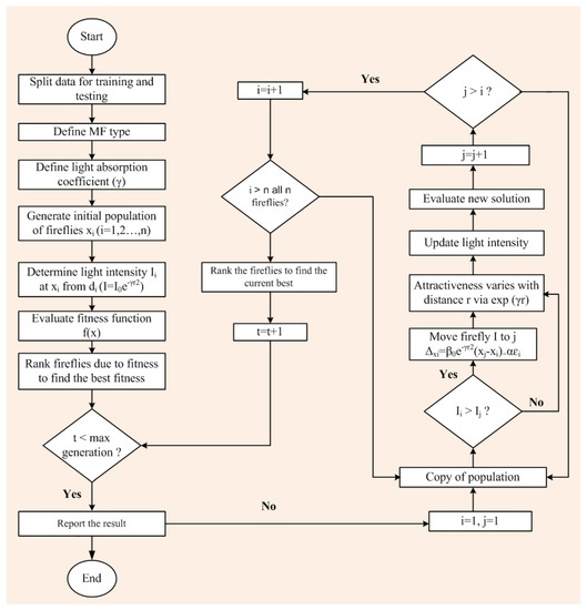 Figure 1. Flow chart of the ANFIS model.
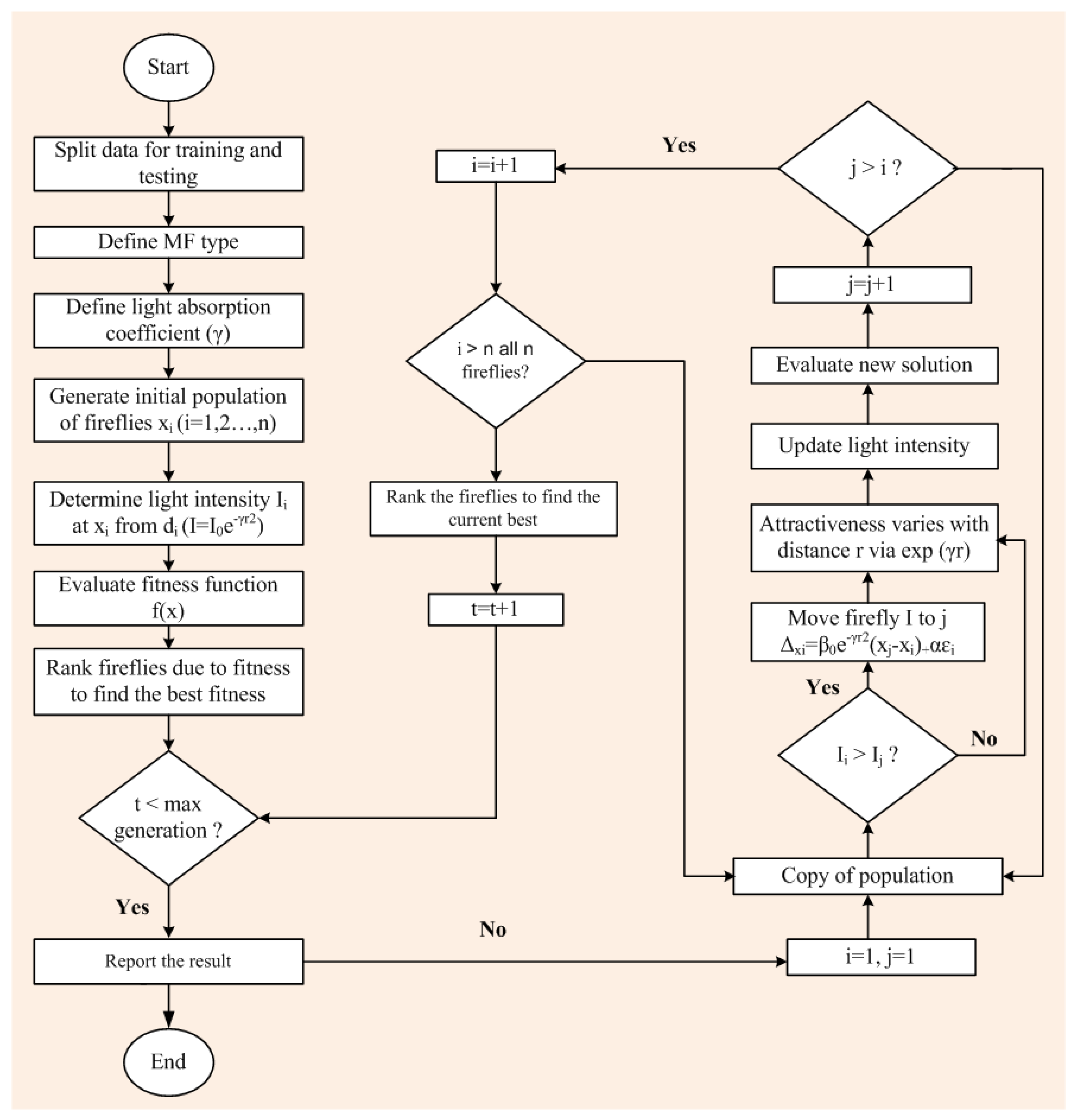
2.2. Firefly Algorithm (FFA)
The mechanism of FFA is based on the nature of the firefly (flashing behavior). This algorithm is applied during the training phase to select the best set of data. This model depends on three basic principles:
- Each firefly can engage another firefly.
- The attractiveness between two fireflies is calculated by the light intensity of each firefly.
- The brightness is correspondingly related to the light released by fireflies [14].
Thus, the objective function of the FFA model is introduced by the intensity of the light produced by, and brightness of, the firefly. The following equations present the intensity (I) and attractiveness, respectively [14,15]:
where r is the distance between fireflies, is light intensity, is attractiveness at r = 0 distance, and is the light absorption coefficient. β and α are the attraction and movement co-efficient. α, β, and are required to be adjusted by trial and error, in order to integrate the ANFIS model with the FFA [14].
2.3. Genetic Algorithm (ANFIS–GA)
This model is highly useful for evapotranspiration calculations. The genetic algorithm (GA) is based on the characters of natural genetics and its selection system. GA includes three major stages: (1) population initialization, (2) GA operators, and (3) evaluation [11]. This system can solve large space problems efficiently and optimize complicated functions. Any hybrid model (hybrid ANFIS) can optimize the MF by using GA. This fuzzy-genetic algorithm has a potential to minimize model errors [11]. The development begins from the population of random chromosomes, thus generating form. In each generation, the fitness of the whole population is estimated. Then, based on the fitness, multiple chromosomes are stochastically adopted from the current population and adjusted by utilizing genetic operators, such as crossover and mutation, to create a new population. The current population is applied in the following iteration of the algorithm [10].
2.4. Particle Swarm Optimization (PSO)
The PSO technique was invented by Kennedy and Eberhart [16], based on the characteristics of bird and fish swarms in a multi-dimensional area, for example, looking for food and running away from hazards [16]. Every element in this algorithm is identified as a “particle”; particles create the density (population), and each density is identified as a “swarm”. Every particle is considered a candidate for the answer to the question in this algorithm. The swarm and particle values of this technique depend on the chromosome and density (population) items, which are similar to the genetic algorithm [12]. PSO is a trial-and-error solution procedure that explores the characteristics of swarm particles in a multi-dimensional exploration zone. The computation process is different in the case of large data sets because of the higher expenses of developing a significant number of models. PSO can optimize with a large possibility and high meeting (convergence) rate. This optimizer works through the following mathematical expression [12].
The values of and are selected according to the limit of the variables. The starting position and velocities of the individuals are irregularly calculated, based on the following equations:
where p, d, v, x, and r denote particle number, exploration direction, particle velocity, position of particle, and irregularly created number close to unvaried distribution with the limit (0, 1), respectively. Each particle upgrades its own position, until the position and velocity values face the stopping condition, based on the earlier steps and position of the finest particle in the entire swarm.
where k indicates the number of repetitions needed for the trial-and-error process. ω, , and are explore variables; and are two irregular numbers with an unvaried distribution with the limit (0, 1). is the finest location defined by a particle, while is the finest location defined by the entire swarm. Variables and are the cognition and social variables, respectively [16]. Kennedy and Eberhart introduced ω as a coefficient, which is 1 in the PSO algorithm.
and k are the highest and current number of repetitions for the trial-and-error process, respectively. Regeneration is chosen with the utilization of linear fitness scaling (LFS) to increase diversity of the iteration process.
where and represent the finest and the least objective functions in the entire swarm and is the expression for diversity. The following equation presents the objective function.
where is observed, and is the estimated evaporation intensity; N is the observation number. This optimization process with the particle swarm technique extends up to a required concluding situation. In this analysis, the aim of the PSO algorithm is to minimize the objective function. The levels of computation of this process, using PSO, can be found in reference [12].
3. Results and Discussion
3.1. Data Description
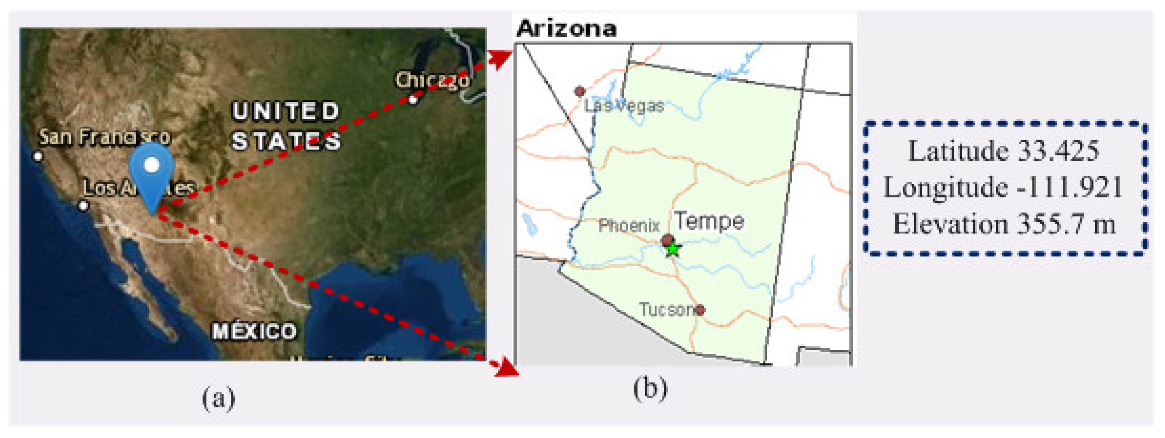
Arizona is the sixth biggest state of USA, which is situated next to the state of California. The area of this state is 113,000 square miles and partly surrounded by the Pacific Ocean. The weather conditions in Arizona are quite caustic, with tropical summers and muggy winters. Phoenix is the capital of Arizona state, located in the Northeastern part of the Sonoran Desert; therefore, it has a hot desert climate condition. This city has an agricultural neighborhood, which is close to the confluence of the Salt and Gila River. The study area was chosen due to the hot climate condition and proximity to an agricultural neighborhood. Figure 2 shows the study area, which is 355.7 m higher from sea level, with 33.4258 latitude and −111.9217 longitude.
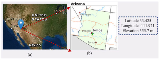
Figure 2.
Location of the study area under consideration in this manuscript. (a) zoom-out view; (b) zoom-in view. Source: Internet.
To assess efficiency, all models are separately calibrated, with a total of 86 data points for an eight-year period of 2010–2017 at each selected station within the United States of America and a one-month lead time. Data were collected from the government database of Arizona state in the US. Study area is humid and has an agricultural neighborhood. Two combinations of data sets were studied to check the results and verify whether they are similar in pattern or not. The data set is initially divided into two parts: the training and test portions. About one-third (~27) of the data points of the total data set was selected as the training data set, whereas the remaining two-thirds (~59) of the data points was considered a testing data set.
Table 1 summarizes the statistical indices of the test, training and all data used in this study. The table contains the skewness, kurtosis, coefficient of variation (CV), standard deviation (SD), and first (1st) and third (3rd) quarters (Q) for all the data points (N). The table also reports the minimum (Min) and maximum (Max), along with the average (Avg), of all data point. It further reports the similar statistical indices for both the training and testing cases, as well.

Table 1.
Statistical indices of the evaporation data set used to verify the modelling.
Standard deviation shows the distribution nature of data set. For example, the standard deviation of the test data set is 82.40, and the average value of the data is 158.73. This means that most of the test data lies between 78.33 (158.73 − 82.40 = 78.33) to 241.13 (158.73 + 82.40 = 241.13). On the other hand, the coefficient of variation shows the precision of the data set in this table. It is defined as the ratio of standard deviation and mean value (in percentages). Two combinations of the testing and training data were chosen arbitrarily, in order to verify the robustness and repeatability of the proposed modeling techniques.
Combination 1: Training data (September 2010 to September 2015); testing data (October 2015 to December 2017).
Combination 2: Training data (September 2010 to December 2012 & June 2015 to December 2017); testing data (January 2013 to May 2015).
3.2. Model Accuracy Indicator
The performances of all four models were individually evaluated using statistical analysis to monitor accuracy, with respect to the evaporation forecasting data. The accuracy indicators for the ANFIS, FFA, PSO, and GA models were calculated, in terms of the coefficient of determination () [17], Nash–Sutcliffe coefficient (NSE) [17], root mean square error (RMSE) [10], mean absolute error (MAE) [17], variance account for (VAF) [18], absolute relative error (MARE), scatter index (SI) [17], bias [13], and root mean square relative error (RMSRE) [17]. The root mean squared error (RMSE) represents a good measure of the goodness of fit at high parameter values. The standard RMSE value should be 0, according to the theory. The relative error (MARE) provides a more balanced idea of the goodness of fit at moderate and low values. The standard value of MARE is also 0. The coefficient of determination should be 1 for a perfect fit model. This coefficient measures the correlation of the predicted values with the observational data—the closer the coefficient is to one, the greater the correlation. The value of this coefficient does not interfere with the data unit considered. The SI index is the relative form of RMSE. The performance factor of the model, expressed as the Nash–Sutcliffe error criterion (), was used to evaluate the predictive power of the model. A value of unity for the indicates optimum conformity between predicted and observed data. In this work, both and are expressed in percentages. The closer their magnitude to 100, the better the performance of the model. The ideal value for VAF is 100. All of them can be calculated from designed formulations, which are presented in the appendices section (see Appendix A for details).
3.3. Simulation Results
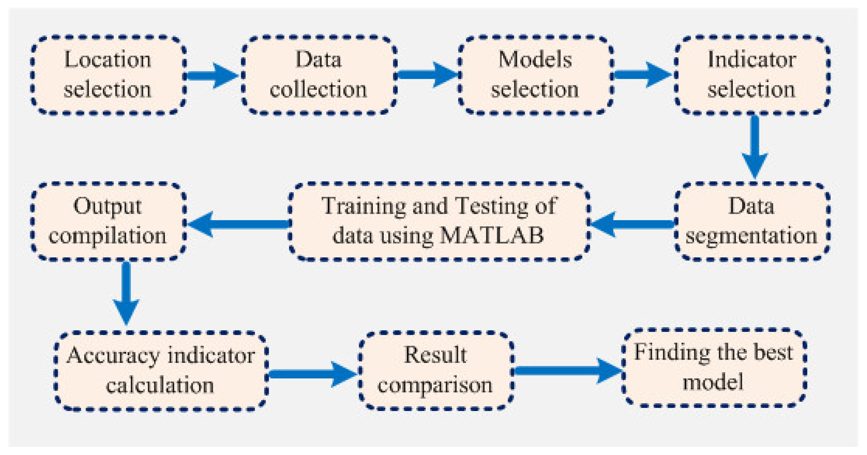
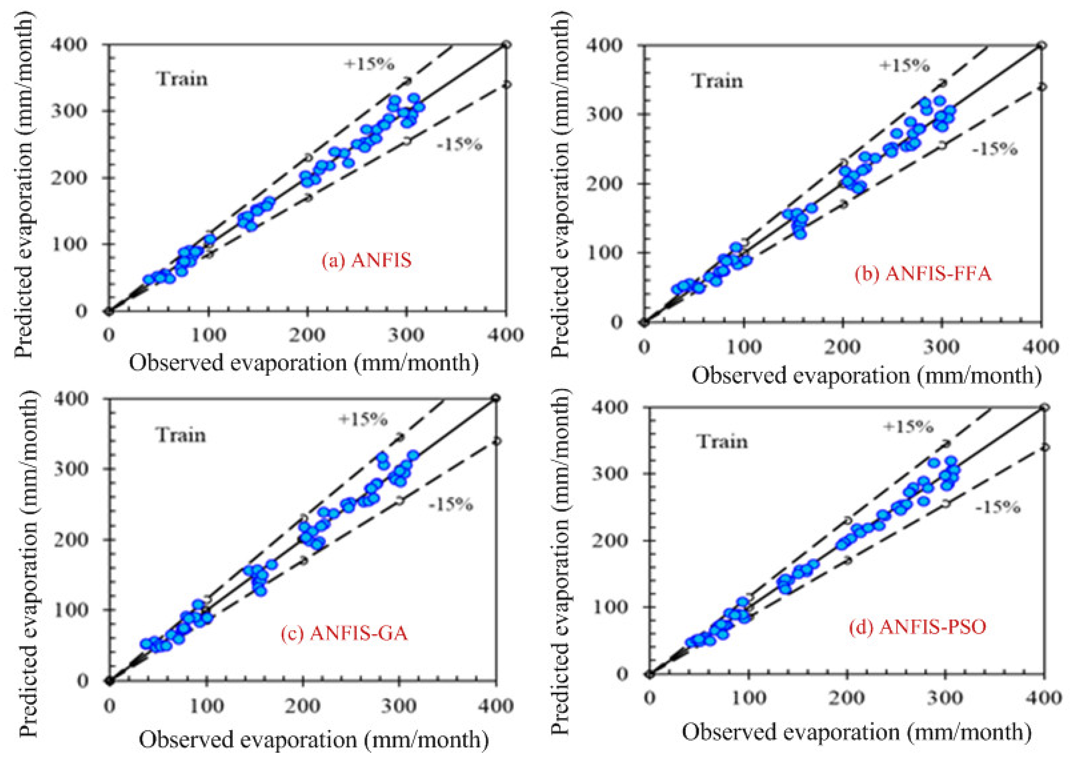
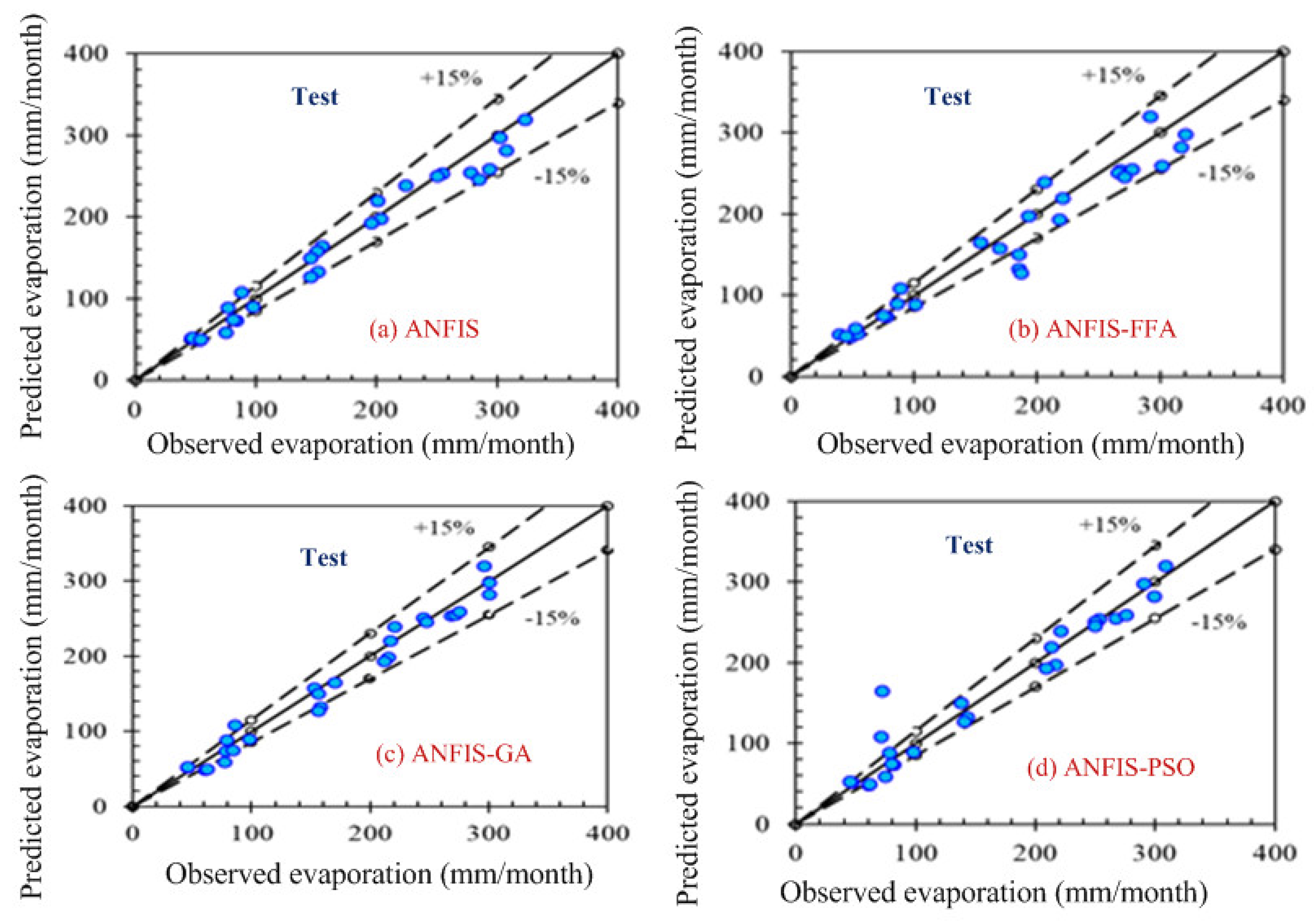
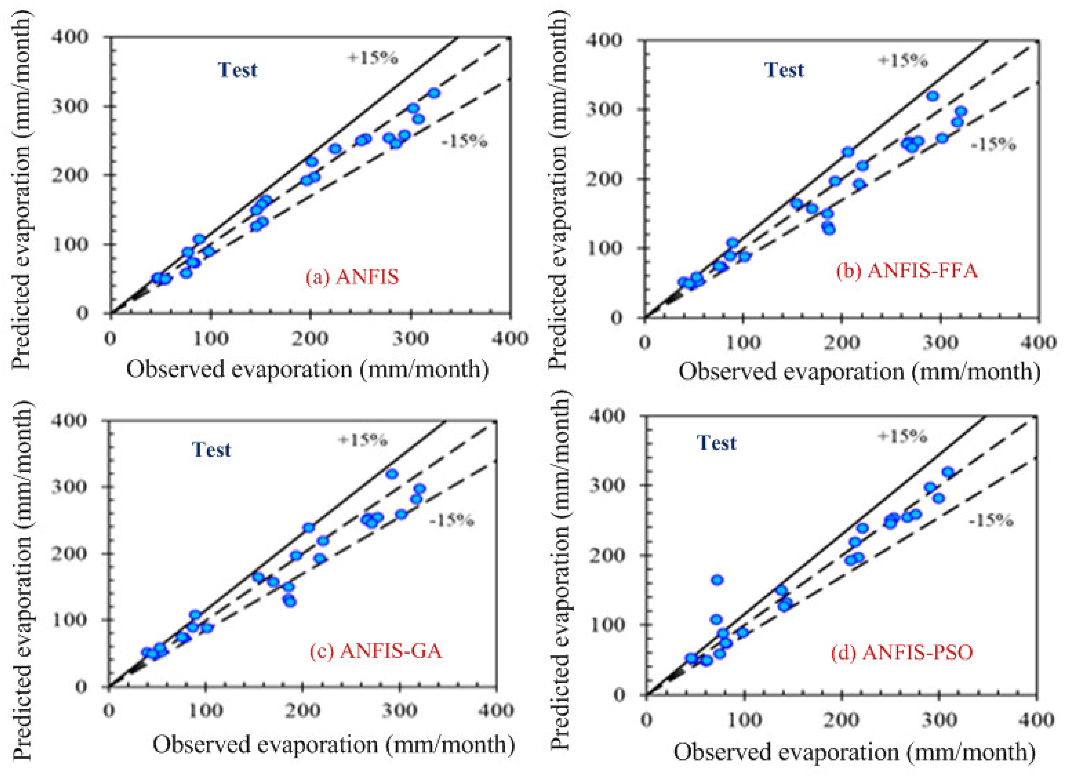
Computer-based software simulation is performed to validate the proposed model; in particular, MATLAB is used to validate the model. Figure 3 shows the step-by-step work, performed in this manuscript, to validate the proposed model. First of all, the data is collected from the location under interest. Secondly, the models are chosen based on the collected data. In this case, ANFIS is chosen due to the nonlinear nature of the data set. Model accuracy indicators are then selected. On the other hand, the data is partitioned in to two groups: one group (almost two third of the data) is for testing the network, while the other group (remaining data set) is for training the proposed model. In the beginning the network is trained using nearly two-thirds of the total data set. This calibrates the network. Later, the remaining data set (approximately one third) are used to test the network. To verify the overall performance of the observed models, the observed and predicted evaporation values were plotted together for both combinations (combinations 1 and 2, as depicted in Section 3.1). Graphical representation is made in terms of the observed and predicted data. Figure 4, Figure 5, Figure 6 and Figure 7 show the pattern of the observed and predicted data for all four models. Figure 4 and Figure 5 show the training data pattern for the first and second combination of data sets as mentioned in Section 3.1. These figures show the comparison of target and output sample index of trained data for the (a) ANFIS, (b) FFA, (c) GA, and (d) PSO models. Similarly, Figure 6 and Figure 7 show the test data pattern of all models, and these present the comparison of the target and obtained output sample index of test data for (a) ANFIS, (b) FFA, (c) GA, and (d) PSO, respectively.
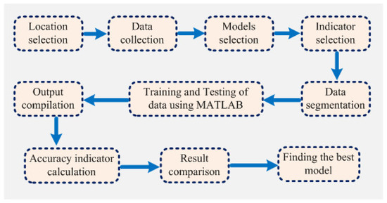
Figure 3.
The step-by-step structural outline of the work performed in this manuscript.
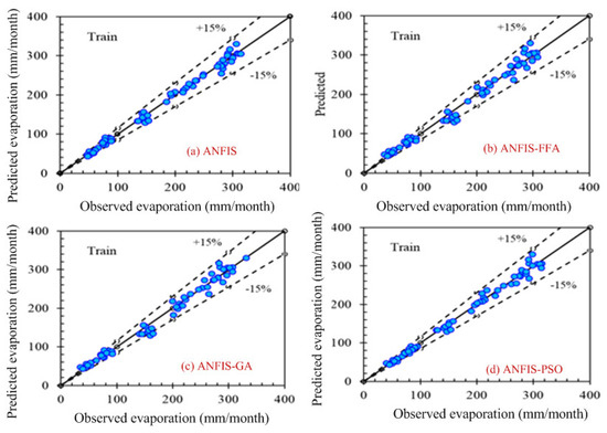
Figure 4.
Comparison of the target (predicted) and obtained output sample index of training data set for (a) ANFIS, (b) ANFIS–FFA, (c) ANFIS–GA, and (d) ANFIS–PSO, respectively, using the first combination of the data set.
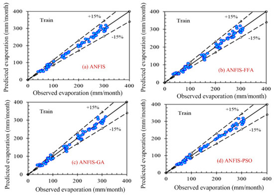
Figure 5.
Comparison of the target (predicted) and obtained output sample index of training data set for (a) ANFIS, (b) ANFIS–FFA, (c) ANFIS–GA, and (d) ANFIS–PSO, respectively, using the second combination of the data set.
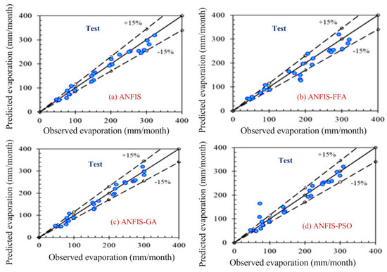
Figure 6.
Comparison of the target and obtained output sample index of the test data for (a) ANFIS, (b) ANFIS–FFA, (c) ANFIS–GA, and (d) ANFIS–PSO, respectively (first combination of the data set).
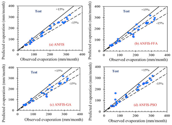
Figure 7.
Comparison of the target and obtained output sample index of the test data for (a) ANFIS, (b) ANFIS–FFA, (c) ANFIS–GA, and (d) ANFIS–PSO, respectively (second combination of the data set).
According to the graphs, both data sets lie between −15% to +15% of a perfect line. Graphical presentation also demonstrates that the data set are well-trained. According to the analysis, all the models are suitable for the evaporation estimation. However, the pattern for Figure 6a ANFIS (first combination) and Figure 7a ANFIS (second combination) were the best fits, and the pattern for Figure 6b ANFIS–FFA (first combination) and Figure 7b ANFIS–FFA (second combination) show less fitness among the four models. The figures for ANFIS–PSO and ANFIS–GA, for both combinations, were close to each other. Additionally, a few accuracy tests were performed to obtain a better understanding for both training and testing. Few statistical indices tests have been performed and summarized in Table 2, Table 3, Table 4, Table 5 and Table 6.
Table 2.
Summary of model accuracy indicator test for the training data set (for the first combination data set), which was calculated in Excel.
Table 3.
Summary of model accuracy indicator test for the testing data set (for the first combination data set), which was calculated in Excel.
Table 4.
Summary of model accuracy indicator test for the training data set (for the second combination data set), which was calculated in Excel.
Table 5.
Summary of model accuracy indicator test for test data set (for the second combination data set), which was calculated in Excel.
Table 6.
Summary of model accuracy indicator test during the testing period, provided by ‘MATLAB’.
The overall summary of the findings is presented in Table 6. Table 6 presents the results provided by the MATLAB tool. It shows that the MSE values, for all the test models, were very high (MSE for ANFIS 241.72, for FFA 594.80, for GA it is 206.79, and for PSO it is 213.05) for the testing data, and higher for the training data. To ensure a rigorous comparison of the models, an extended analysis was performed using RMSE, , MAE, MARE, RMSRE, SI, MRE, Bias, NASH, and VAF as statistical indices for the estimated values. Table 2, Table 3, Table 4 and Table 5 present values of all statistical indices for training and testing data set of all models. According to all statistical indices, especially the , RMSE, VAF, and NASH values, the second combination of the data set presented better results than the first combination of the data set, which is presented in Table 3. The results of the ANFIS and ANFIS–PSO models were almost identical in both combinations. RMSE was lower for ANFIS and ANFIS–GA. ANFIS–FFA posed worse results, among all model, in all the cases. Biasness is less for ANFIS model. According to the test results from Table 3 and Table 5, the for ANFIS, GA, and PSO were almost identical, 0.99, whereas for FFA was 0.97. This is found to be aligned with the training result. A commonly used correlation measure, i.e., (), in the testing of statistical indices cannot always be accurate, or sometimes it could be misleading, when used to compare the predicted and observed models [1]. The two most widely used statistical indicators, i.e., root mean square error (RMSE) and bias error, were used in this analysis. The model performance is inversely proportional to the RMSE value; lower RMSE values present higher accuracy and vice versa. RMSE is the minimum for PSO and GA, which were 14.59, 14.63, and 14.38, 15.07, respectively, whereas ANFIS was 15.54, and FFA presents the worst value: 24.38. Negative biasness was noticed for all the models, where ANFIS and GA possessed minimum biasness.
Hence, the MSE values are higher, and the relative statistical indices are compared to find better results. The MARE and RMSRE results should also be minimal for the best fit model. Again, ANFIS shows the minimum MARE value (0.087), and PSO gives similar result to ANFIS. However, according to the RMSRE results, PSO shows the best result. For more clarity, NASH has been considered another accuracy indicator, and the value should be close to 1 for the best fit. The table presents the highest NASH value for ANFIS (0.97), GA (0.97), and PSO (0.97). FFA was also close to 1 (0.93). To avoid confusion, VAF was calculated. Here, ANFIS, GA, and PSO showed higher results (all three results were close to 97.11), and FFA indicates 93.11.
Time is an important factor of these calculations. The time frame is given below in Table 7 for all four models. It shows that the ANFIS model took less time than the others, and FFA is the complicated one. After analyzing all the results, the FFA model is considered the least acceptable model among the four. ANFIS, with GA and PSO models, were showing better fit in some situations. Although GA and PSO were showing similar results and took same time to run, ANFIS can be considered more acceptable because of its simplicity.
Table 7.
Time taken by four models (approximate).
3.4. Discussion
In this study, evaporation was estimated from six climate variables, i.e, minimum temperature, maximum temperature, average temperature, sunshine hour, wind speed, and relative humidity. Evaporation depends on the combined effect of humidity, temperature variation, sunshine, and wind [11]. Sunshine is an important factor that helps evaporate the water body [7]. Similarly, temperature and humidity also play an important role in evaporation. When they decrease, evaporation increases. Wind takes water away to the atmosphere [7]. Therefore, all of them were considered, as they affect evaporation. Key parameters were selected by trial-and-error method. Only one set of parameters was experimented with.
The findings of this research demonstrated that the FFA model is considered the least acceptable model among the four. ANFIS with GA and PSO models were showing a better fit in some situations. Although GA and PSO were showing similar results, based on all accuracy indicator tests (especially, on maximum value, minimum RMSE, less Biasness, maximum VAF, minimum RMSRE value, and maximum value of Nash coefficient), and took the same time to run the model, ANFIS can be considered more acceptable because of its simplicity. This model can be used as a role model for any dataset of an arid climate. It can be helpful for the local stakeholder, in terms of the hydrological resource management system. The main advantage of adopting ANFIS for this location is the pattern of the dataset. As the datasets are inherently nonlinear, the ANFIS model was able to achieve high accuracy in the prediction of evaporation. The ANFIS model and this model, with the optimizers (FFA, GA, and PSO), can be widely used for arid climates, with the same weather variables, in any part of the world.
More investigation is needed for this location. Lack of data was a limitation of this study. More climate variables can be added for more accuracy of the model. Other modern machine learning technique should be implemented in the future, in order to use the available resources to enhance the water resource management system. That would be beneficial for the local agri-economical prospect, as well.
4. Conclusions
The comparison among the adaptive neuro fuzzy inference system (ANFIS) and its hybridization, using three different algorithms (FFA, GA, and PSO), has been illustrated in this study, in the context of evaporation estimation, using different climate variables, namely sunshine, relative humidity, average temperature, maximum temperature, minimum temperature, and wind speed. Two combinations of data sets were trained and tested, in order to verify the correlation among the different models. The study illustrated the accuracy of all four models. However, the performance of the models was evaluated based on the various statistical measures (RMSE, RMSRE, MBE, VAF, NASH, biasness, MBE, MARE, SI, and ). Result shows that the second combination of the testing and training data set posed slightly better results than the first combination. Overall, all four models are suitable for the estimation of evaporation, but ANFIS and ANFIS, with optimizer PSO, is superior for all accuracy indicator values. Relative and absolute accuracy tests were performed to find the best model in this study. Though all the results of the two models (ANFIS and ANFIS–PSO) were merely identical, ANFIS is recommended, due to its simple formulation and easy development, compared to the ANFIS–PSO model. The computational time of ANFIS model is less, in comparison to the other models with optimizers. The main objective of the adoption of different optimizer techniques is to verify the accuracy of the outcome prediction by ANFIS model. Since the prediction was almost identical in all cases, the ANFIS model is recommended, due to its simplicity. The major challenge of this project was the limitation of data. These models can be applied for different data sets to investigate the results, if they were available. This analysis is limited to a particular location. However, in future work, other locations can be explored, and their performance can be compared with modern machine learning methods. Another optimizer, for example, the ant colony optimizer (ACO), can be investigated in future work. Multi gene-genetic programming (MGGP) can also be explored in the future. Another climate variable, such as, atmospheric pressure, can be considered as an input in the future. However, the evaporation of a given location can easily be modelled from the available data using the ANFIS model. Additionally, this model can be applied as a module for calculating evaporation data in hydrological modeling studies.
Author Contributions
Conceptualization, M.J., H.B., and A.M.; methodology, M.J. and H.B.; software, A.M.; validation, M.J.; formal analysis, M.J. and A.M.; investigation, M.J.; resources, H.B.; data curation, M.J. and H.B.; writing—original draft preparation, M.J.; writing—review and editing, H.B. and A.M.; visualization, H.B.; supervision, A.M.; project administration, H.B. All authors have read and agreed to the published version of the manuscript.
Funding
This research received no external funding.
Data Availability Statement
Part of the data used in this manuscript are available through the corresponding author upon reasonable request.
Acknowledgments
Mansura Jasmine acknowledges the support of Mehedi Hasan during the preparation of this manuscript.
Conflicts of Interest
The authors declare no conflict of interest.
Appendix A
The relationships for statistical indices and error measures used in this paper are provided in the following.
: coefficient of determination, which can be expressed in the following form:
RMSE: root mean square error, which can be formulated as follows:
MARE: absolute relative error. The formula is given below:
SI: scatter index, which can be expressed as follows:
RMSRE: root mean square relative error. This error can be calculated from the following equation:
MAE: mean absolute error. This error can be calculated from the following equation:
VAF: variance account for. This term can be presented by the following equation:
NSE: Nash–Sutcliffe coefficient. This coefficient can be formulated as follows:
where,
- : the output observational parameter;
- : the y parameter predicted by the models;
- : the mean predicted y parameter;
- M: the number of parameters;
- n: number of samples;
- : the Nash–Sutcliffe test statistic;
- : the ith value of actual data;
- : the ith value of predicted data.
References
- Benzagtha, M.A. Estimation of Evaporation from a Reservoir in Semi-arid Environments Using Artificial Neural Network and Climate Based Models. Br. J. Appl. Sci. Technol. 2014, 4, 3501–3518. [Google Scholar] [CrossRef]
- Dogana, E.; Gumrukcuoglu, M.; Sandalci, M.; Opan, M. Modelling of evaporation from the reservoir of Yuvacik dam using adaptive neuro-fuzzy inference systems. Eng. Appl. Artif. Intell. 2010, 23, 961–967. [Google Scholar] [CrossRef]
- Kisi, O.; Sanikhani, H.; Zounemat-Kermani, M. Comparison of two different adaptive Neuro-Fuzzy inference system in modelling daily reference evapotranspiration. Water Resour. Manag. 2014, 28, 2655–2675. [Google Scholar] [CrossRef]
- Kisi, O.; Sanikhani, H.; Zounemat-Kermani, M.; Niazi, F. Long-term monthly evaporation modeling by several data-driven methods without climate data. Comput. Electron. Agric. 2015, 115, 66–77. [Google Scholar] [CrossRef]
- Moghaddamnia, A.; Gousheh, M.G.; Pirli, J.; Amin, S.; Han, D. Evaporation estimation using artificial neural network and adaptive neuro-fuzzy inference system techniques. Adv. Water Resour. 2009, 32, 88–97. [Google Scholar] [CrossRef]
- Goyal, M.K.; Bharti, B.; Quilty, J.; Adamowsky, J.; Pandey, A. Modeling of daily pan evaporation in subtropical climates using ANN, LS-SVR, Fuzzy Logic, and ANFIS. Expert Syst. Appl. 2014, 41, 5267–5276. [Google Scholar] [CrossRef]
- Malik, A.; Tikhamarine, Y.; Al-Ansari, N.; Shahid, S.; Sekhon, H.S.; Pal, R.K.; Rai, P.; Panday, K.; Singh, P.; Elbeltagi, A.; et al. Daily pan evaporation estimation in different agro-climatic zones using hybrid support vector regression optimized by Salp swarm algorithm in conjunction with gamma test. Eng. Appl. Comput. Fluid Mech. 2021, 15, 1075–1094. [Google Scholar] [CrossRef]
- Malik, A.; Saggi, M.K.; Rehman, S.; Sajjad, H.; Inyurt, S.; Bhatia, A.S.; Farooque, A.A.; Oudah, A.Y.; Yaseen, Z.M. Deep learning versus gradient boosting machine for pan evaporation prediction. Eng. Appl. Comput. Fluid Mech. 2022, 16, 570–587. [Google Scholar] [CrossRef]
- Malik, A.; Kumar, A.; Kimb, S.; Kashani, H.M.; Karimi, V.; Sharafati, A.; Ghorbani, A.M.; Al-Ansari, N.; Salih, S.Q.; Yaseen, Z.M.; et al. Modeling monthly pan evaporation process over the Indian central Himalayas: Application of multiple learning artificial intelligence model. Eng. Appl. Comput. Fluid Mech. 2020, 14, 323–338. [Google Scholar] [CrossRef] [Green Version]
- Ayvaz, M.T.; Elci, A. Identification of the optimum groundwater quality monitoring network using a genetic algorithm-based optimization approach. J. Hydrol. 2018, 563, 1078–1091. [Google Scholar] [CrossRef]
- Wang, L.; Kisi, O.; Sanikhani, H.; Zounemat-Kermani, M.; Li, H. Pan evaporation modelling six different heuristic computing methods in different climates in China. J. Hydrol. 2017, 544, 407–427. [Google Scholar] [CrossRef]
- Karahan, H. Determining rainfall-intensity-duration-frequency relationship using particle swarm optimization. J. Civil Eng. 2012, 16, 667–675. [Google Scholar] [CrossRef]
- Chang, F.J.; Chang, Y.T. Adaptive neuro-fuzzy inference system for prediction of water level in reservoir. Adv. Water Resour. 2006, 29, 1–10. [Google Scholar] [CrossRef]
- Yaseen, Z.M.; Ebtehaj, I.; Bonakdari, H.; Deo, R.C.; Mehr, A.D.; Mohtar, W.H.M.W.; Diop, L.; El-Shafie, A.; Singh, V.P. Novel approach for streamflow forecasting using a hybrid ANFIS-FFA model. J. Hydrol. 2017, 554, 263–276. [Google Scholar] [CrossRef]
- Yaseen, Z.M.; Ghareb, M.I.; Ebtehaj, I.; Bonakdari, H.; Siddique, R.; Heddam, S.; Yusif, A.A.; Deo, R. Rainfall pattern forecasting using novel hybrid intelligent model based ANFIS-FFA. Water Resour. Manag. 2018, 32, 105–122. [Google Scholar] [CrossRef]
- Kennedy, J.; Eberhart, R.C. Particle swarm optimization. In Proceedings of the IEEE international Conference on Neural Networks, Perth, Australia, 27 November–1 December 1995; pp. 1942–1948. [Google Scholar]
- Lotfi, K.; Bonakdari, H.; Ebtehaj, I.; Mjalli, S.F.; Zeynoddin, M.; Delatolla, R.; Gharabaghi, B. Predicting wastewater treatment plant quality parameters using a novel hybrid linear-nonlinear methodology. J. Environ. Manag. 2019, 240, 464–474. [Google Scholar] [CrossRef] [PubMed]
- Zeynoddin, M.; Bonakdari, H.; Ebtehaj, I.; Esmaeilbeiki, F.; Gharabaghi, B.; Zare Haghi, D. A reliable schochastic daily soil temperature forecast model. Soil Tillage Res. 2019, 189, 73–87. [Google Scholar] [CrossRef]

Publisher’s Note: MDPI stays neutral with regard to jurisdictional claims in published maps and institutional affiliations. |
© 2022 by the authors. Licensee MDPI, Basel, Switzerland. This article is an open access article distributed under the terms and conditions of the Creative Commons Attribution (CC BY) license (https://creativecommons.org/licenses/by/4.0/).