3.1. Data Description
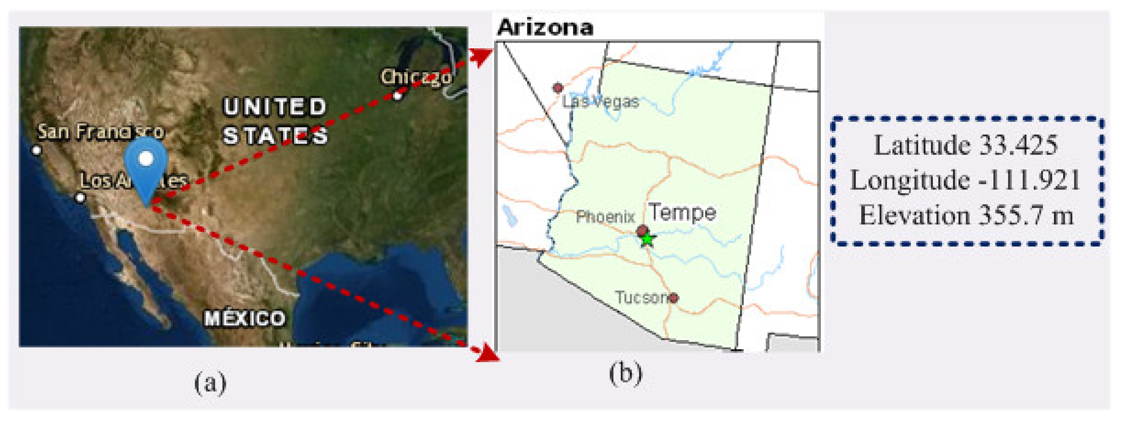
Arizona is the sixth biggest state of USA, which is situated next to the state of California. The area of this state is 113,000 square miles and partly surrounded by the Pacific Ocean. The weather conditions in Arizona are quite caustic, with tropical summers and muggy winters. Phoenix is the capital of Arizona state, located in the Northeastern part of the Sonoran Desert; therefore, it has a hot desert climate condition. This city has an agricultural neighborhood, which is close to the confluence of the Salt and Gila River. The study area was chosen due to the hot climate condition and proximity to an agricultural neighborhood.
Figure 2 shows the study area, which is 355.7 m higher from sea level, with 33.4258 latitude and −111.9217 longitude.
To assess efficiency, all models are separately calibrated, with a total of 86 data points for an eight-year period of 2010–2017 at each selected station within the United States of America and a one-month lead time. Data were collected from the government database of Arizona state in the US. Study area is humid and has an agricultural neighborhood. Two combinations of data sets were studied to check the results and verify whether they are similar in pattern or not. The data set is initially divided into two parts: the training and test portions. About one-third (~27) of the data points of the total data set was selected as the training data set, whereas the remaining two-thirds (~59) of the data points was considered a testing data set.
Table 1 summarizes the statistical indices of the test, training and all data used in this study. The table contains the skewness, kurtosis, coefficient of variation (CV), standard deviation (SD), and first (1st) and third (3rd) quarters (Q) for all the data points (N). The table also reports the minimum (Min) and maximum (Max), along with the average (Avg), of all data point. It further reports the similar statistical indices for both the training and testing cases, as well.
Standard deviation shows the distribution nature of data set. For example, the standard deviation of the test data set is 82.40, and the average value of the data is 158.73. This means that most of the test data lies between 78.33 (158.73 − 82.40 = 78.33) to 241.13 (158.73 + 82.40 = 241.13). On the other hand, the coefficient of variation shows the precision of the data set in this table. It is defined as the ratio of standard deviation and mean value (in percentages). Two combinations of the testing and training data were chosen arbitrarily, in order to verify the robustness and repeatability of the proposed modeling techniques.
Combination 1: Training data (September 2010 to September 2015); testing data (October 2015 to December 2017).
Combination 2: Training data (September 2010 to December 2012 & June 2015 to December 2017); testing data (January 2013 to May 2015).
3.2. Model Accuracy Indicator
The performances of all four models were individually evaluated using statistical analysis to monitor accuracy, with respect to the evaporation forecasting data. The accuracy indicators for the ANFIS, FFA, PSO, and GA models were calculated, in terms of the coefficient of determination (
) [
17], Nash–Sutcliffe coefficient (NSE) [
17], root mean square error (RMSE) [
10], mean absolute error (MAE) [
17], variance account for (VAF) [
18], absolute relative error (MARE), scatter index (SI) [
17], bias [
13], and root mean square relative error (RMSRE) [
17]. The root mean squared error (RMSE) represents a good measure of the goodness of fit at high parameter values. The standard RMSE value should be 0, according to the theory. The relative error (MARE) provides a more balanced idea of the goodness of fit at moderate and low values. The standard value of MARE is also 0. The coefficient of determination
should be 1 for a perfect fit model. This coefficient measures the correlation of the predicted values with the observational data—the closer the coefficient is to one, the greater the correlation. The value of this coefficient does not interfere with the data unit considered. The SI index is the relative form of RMSE. The performance factor of the model, expressed as the Nash–Sutcliffe error criterion (
), was used to evaluate the predictive power of the model. A value of unity for the
indicates optimum conformity between predicted and observed data. In this work, both
and
are expressed in percentages. The closer their magnitude to 100, the better the performance of the model. The ideal value for VAF is 100. All of them can be calculated from designed formulations, which are presented in the appendices section (see
Appendix A for details).
3.3. Simulation Results
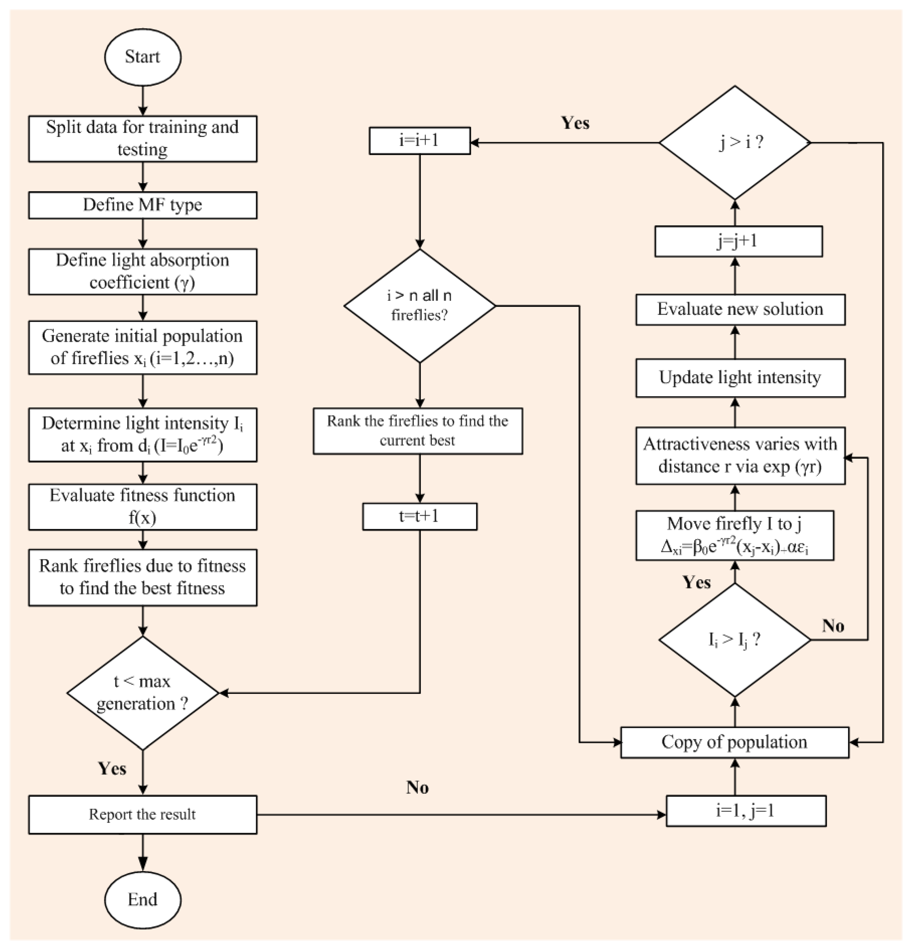
Computer-based software simulation is performed to validate the proposed model; in particular, MATLAB is used to validate the model.
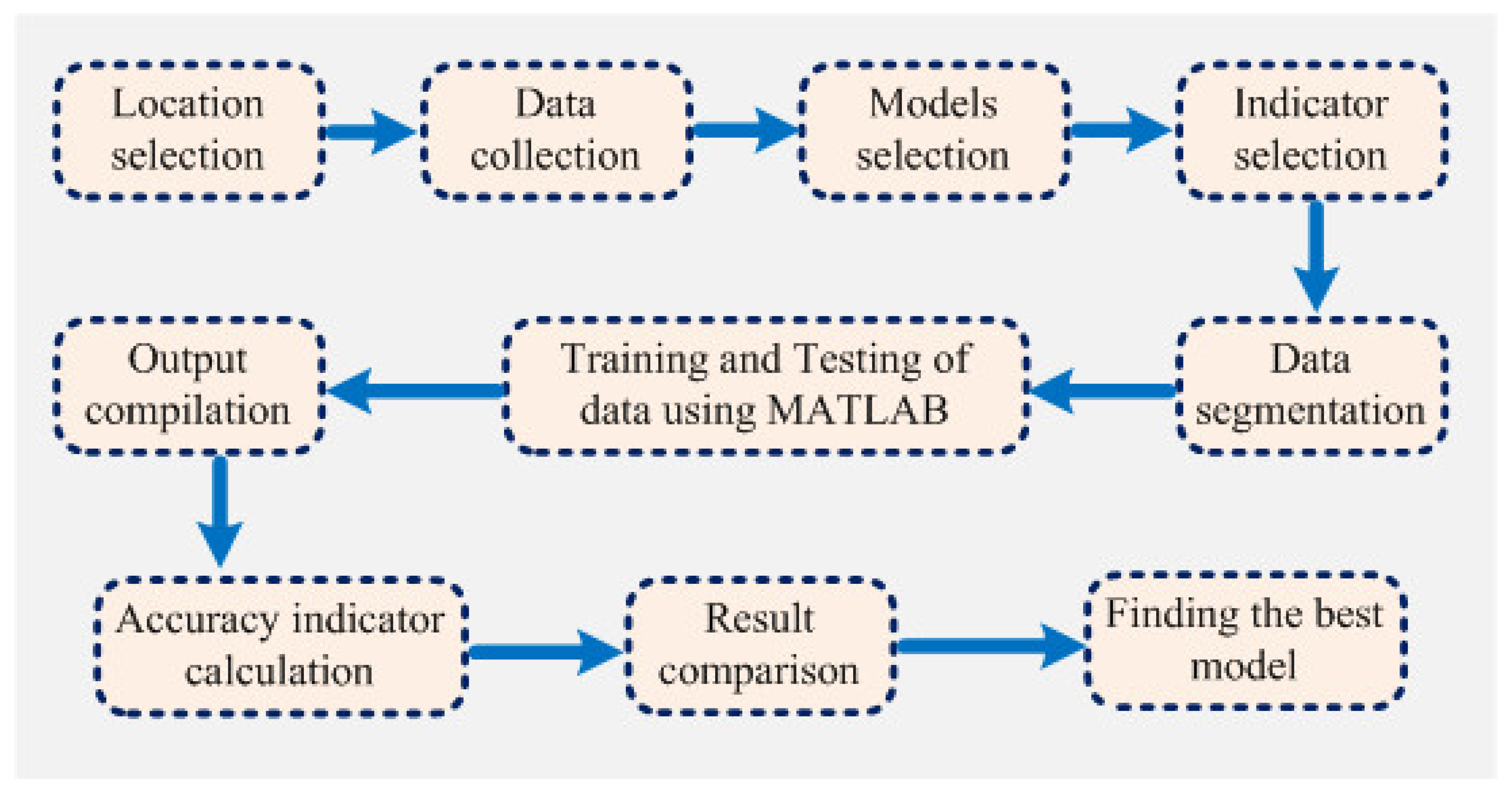
Figure 3 shows the step-by-step work, performed in this manuscript, to validate the proposed model. First of all, the data is collected from the location under interest. Secondly, the models are chosen based on the collected data. In this case, ANFIS is chosen due to the nonlinear nature of the data set. Model accuracy indicators are then selected. On the other hand, the data is partitioned in to two groups: one group (almost two third of the data) is for testing the network, while the other group (remaining data set) is for training the proposed model. In the beginning the network is trained using nearly two-thirds of the total data set. This calibrates the network. Later, the remaining data set (approximately one third) are used to test the network. To verify the overall performance of the observed models, the observed and predicted evaporation values were plotted together for both combinations (combinations 1 and 2, as depicted in
Section 3.1). Graphical representation is made in terms of the observed and predicted data.
Figure 4,
Figure 5,
Figure 6 and
Figure 7 show the pattern of the observed and predicted data for all four models.
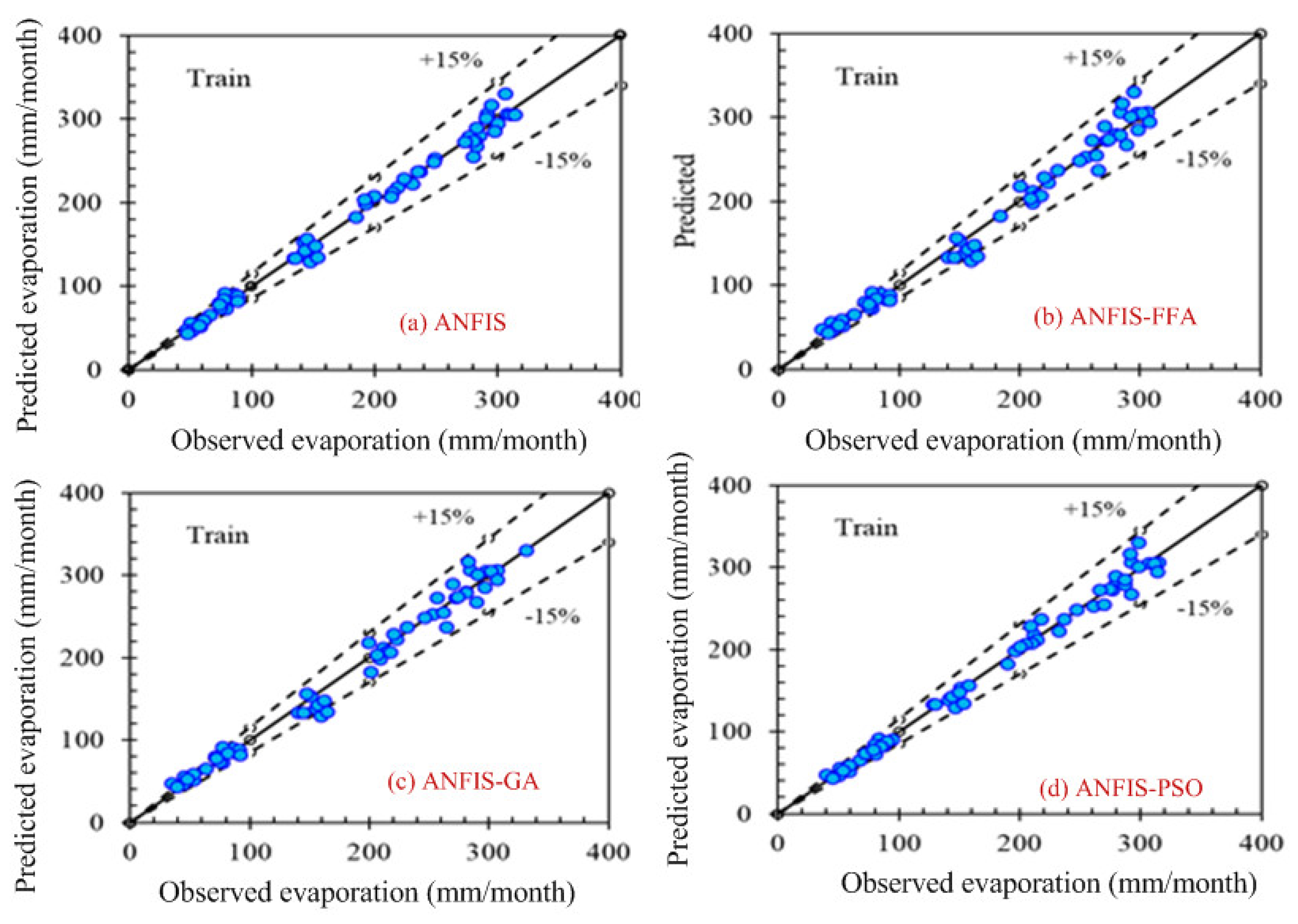
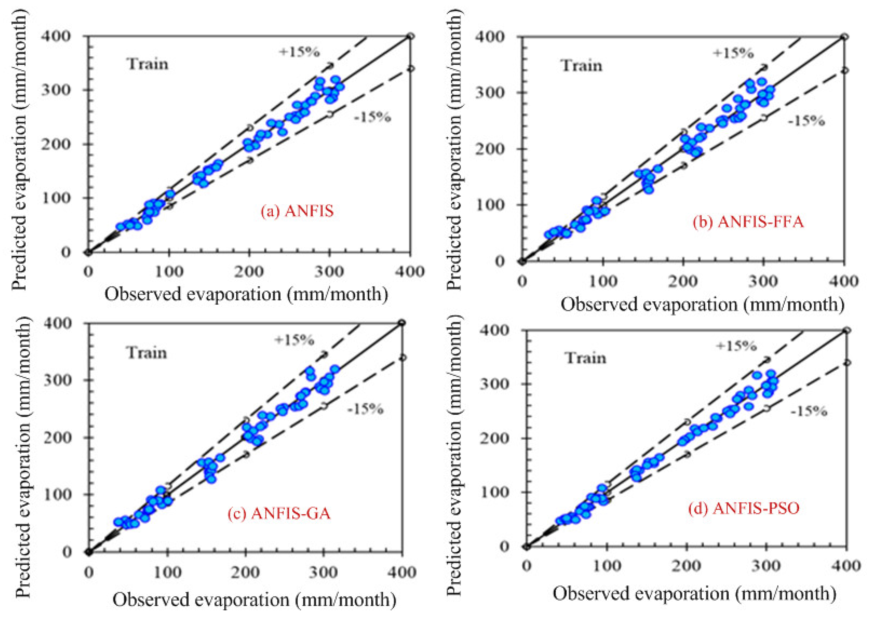
Figure 4 and
Figure 5 show the training data pattern for the first and second combination of data sets as mentioned in
Section 3.1. These figures show the comparison of target and output sample index of trained data for the (a) ANFIS, (b) FFA, (c) GA, and (d) PSO models. Similarly,
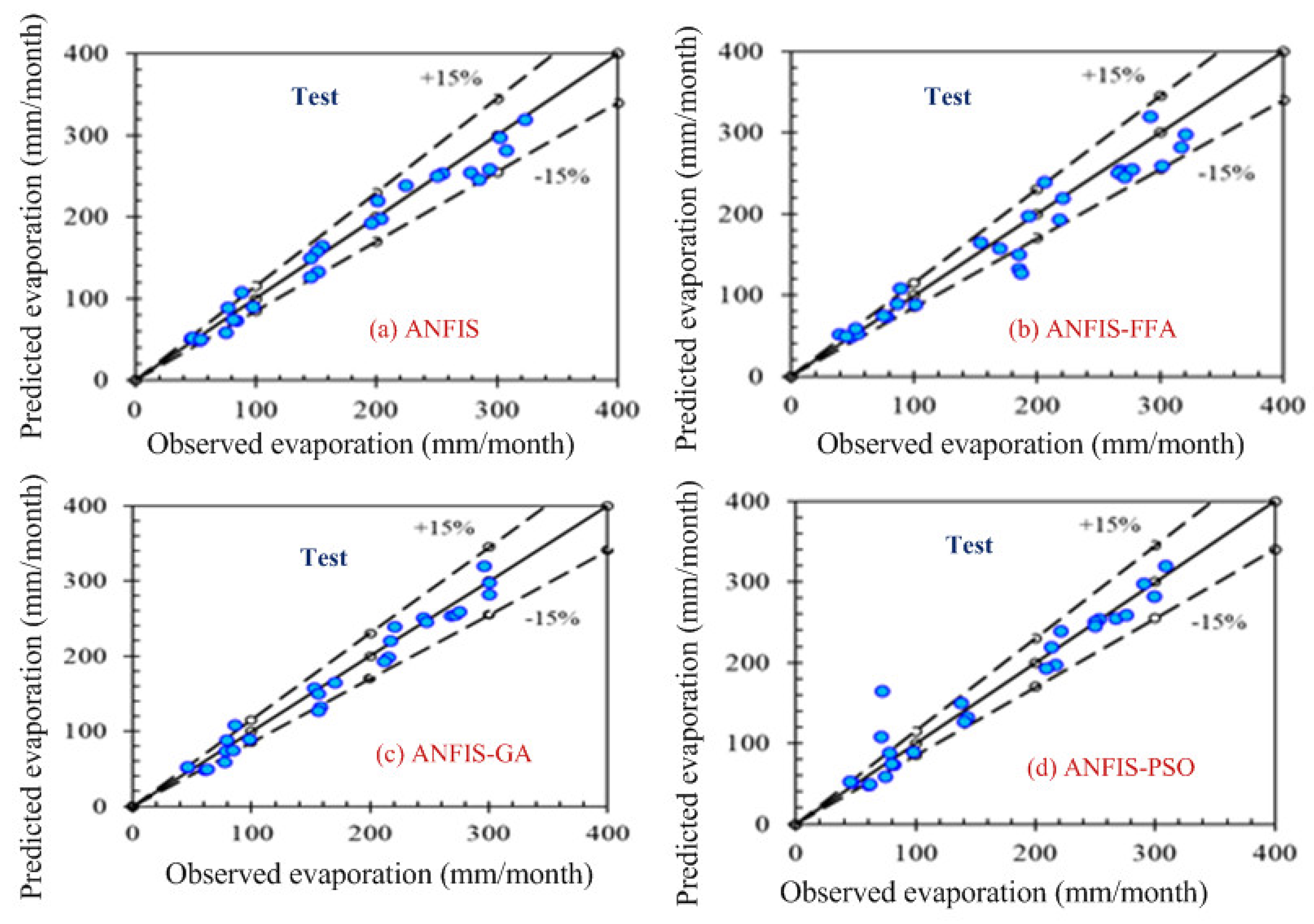
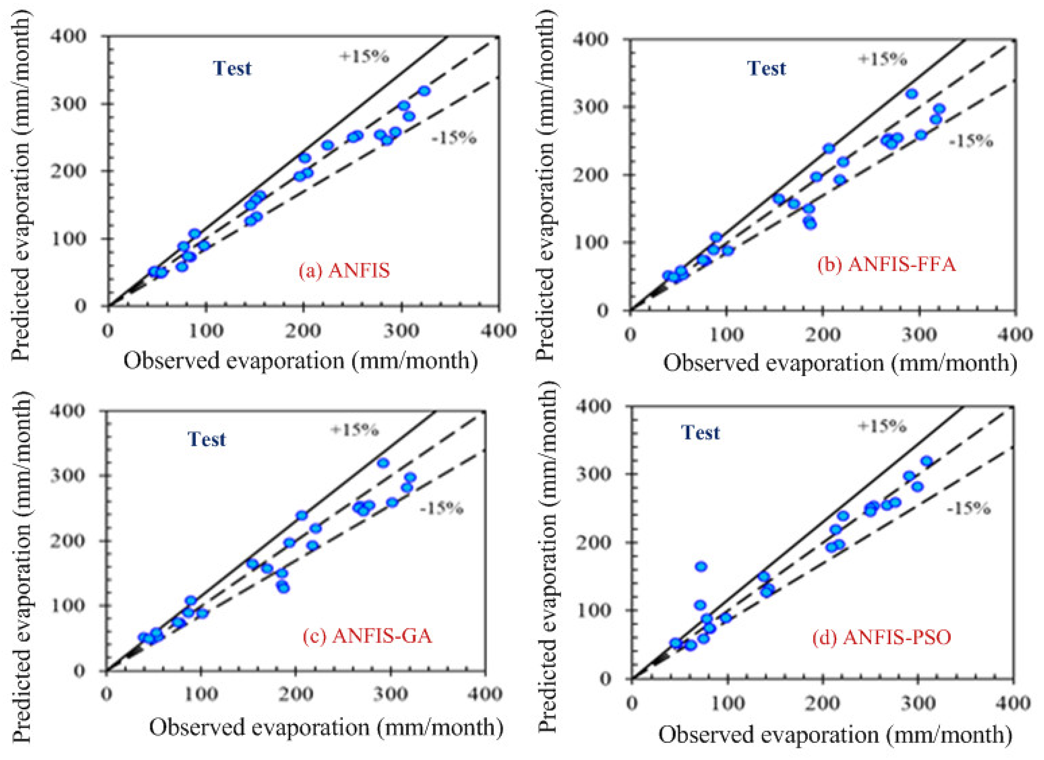
Figure 6 and
Figure 7 show the test data pattern of all models, and these present the comparison of the target and obtained output sample index of test data for (a) ANFIS, (b) FFA, (c) GA, and (d) PSO, respectively.
According to the graphs, both data sets lie between −15% to +15% of a perfect line. Graphical presentation also demonstrates that the data set are well-trained. According to the analysis, all the models are suitable for the evaporation estimation. However, the pattern for
Figure 6a ANFIS (first combination) and
Figure 7a ANFIS (second combination) were the best fits, and the pattern for
Figure 6b ANFIS–FFA (first combination) and
Figure 7b ANFIS–FFA (second combination) show less fitness among the four models. The figures for ANFIS–PSO and ANFIS–GA, for both combinations, were close to each other. Additionally, a few accuracy tests were performed to obtain a better understanding for both training and testing. Few statistical indices tests have been performed and summarized in
Table 2,
Table 3,
Table 4,
Table 5 and
Table 6.
The overall summary of the findings is presented in
Table 6.
Table 6 presents the results provided by the MATLAB tool. It shows that the MSE values, for all the test models, were very high (MSE for ANFIS 241.72, for FFA 594.80, for GA it is 206.79, and for PSO it is 213.05) for the testing data, and higher for the training data. To ensure a rigorous comparison of the models, an extended analysis was performed using RMSE,
, MAE, MARE, RMSRE, SI, MRE, Bias, NASH, and VAF as statistical indices for the estimated values.
Table 2,
Table 3,
Table 4 and
Table 5 present values of all statistical indices for training and testing data set of all models. According to all statistical indices, especially the
, RMSE, VAF, and NASH values, the second combination of the data set presented better results than the first combination of the data set, which is presented in
Table 3. The results of the ANFIS and ANFIS–PSO models were almost identical in both combinations. RMSE was lower for ANFIS and ANFIS–GA. ANFIS–FFA posed worse results, among all model, in all the cases. Biasness is less for ANFIS model. According to the test results from
Table 3 and
Table 5, the
for ANFIS, GA, and PSO were almost identical, 0.99, whereas
for FFA was 0.97. This is found to be aligned with the training result. A commonly used correlation measure, i.e., (
), in the testing of statistical indices cannot always be accurate, or sometimes it could be misleading, when used to compare the predicted and observed models [
1]. The two most widely used statistical indicators, i.e., root mean square error (RMSE) and bias error, were used in this analysis. The model performance is inversely proportional to the RMSE value; lower RMSE values present higher accuracy and vice versa. RMSE is the minimum for PSO and GA, which were 14.59, 14.63, and 14.38, 15.07, respectively, whereas ANFIS was 15.54, and FFA presents the worst value: 24.38. Negative biasness was noticed for all the models, where ANFIS and GA possessed minimum biasness.
Hence, the MSE values are higher, and the relative statistical indices are compared to find better results. The MARE and RMSRE results should also be minimal for the best fit model. Again, ANFIS shows the minimum MARE value (0.087), and PSO gives similar result to ANFIS. However, according to the RMSRE results, PSO shows the best result. For more clarity, NASH has been considered another accuracy indicator, and the value should be close to 1 for the best fit. The table presents the highest NASH value for ANFIS (0.97), GA (0.97), and PSO (0.97). FFA was also close to 1 (0.93). To avoid confusion, VAF was calculated. Here, ANFIS, GA, and PSO showed higher results (all three results were close to 97.11), and FFA indicates 93.11.
Time is an important factor of these calculations. The time frame is given below in
Table 7 for all four models. It shows that the ANFIS model took less time than the others, and FFA is the complicated one. After analyzing all the results, the FFA model is considered the least acceptable model among the four. ANFIS, with GA and PSO models, were showing better fit in some situations. Although GA and PSO were showing similar results and took same time to run, ANFIS can be considered more acceptable because of its simplicity.
3.4. Discussion
In this study, evaporation was estimated from six climate variables, i.e, minimum temperature, maximum temperature, average temperature, sunshine hour, wind speed, and relative humidity. Evaporation depends on the combined effect of humidity, temperature variation, sunshine, and wind [
11]. Sunshine is an important factor that helps evaporate the water body [
7]. Similarly, temperature and humidity also play an important role in evaporation. When they decrease, evaporation increases. Wind takes water away to the atmosphere [
7]. Therefore, all of them were considered, as they affect evaporation. Key parameters were selected by trial-and-error method. Only one set of parameters was experimented with.
The findings of this research demonstrated that the FFA model is considered the least acceptable model among the four. ANFIS with GA and PSO models were showing a better fit in some situations. Although GA and PSO were showing similar results, based on all accuracy indicator tests (especially, on maximum value, minimum RMSE, less Biasness, maximum VAF, minimum RMSRE value, and maximum value of Nash coefficient), and took the same time to run the model, ANFIS can be considered more acceptable because of its simplicity. This model can be used as a role model for any dataset of an arid climate. It can be helpful for the local stakeholder, in terms of the hydrological resource management system. The main advantage of adopting ANFIS for this location is the pattern of the dataset. As the datasets are inherently nonlinear, the ANFIS model was able to achieve high accuracy in the prediction of evaporation. The ANFIS model and this model, with the optimizers (FFA, GA, and PSO), can be widely used for arid climates, with the same weather variables, in any part of the world.
More investigation is needed for this location. Lack of data was a limitation of this study. More climate variables can be added for more accuracy of the model. Other modern machine learning technique should be implemented in the future, in order to use the available resources to enhance the water resource management system. That would be beneficial for the local agri-economical prospect, as well.


