The Sine Modified Lindley Distribution

Abstract

The paper contributes majorly in the development of a flexible trigonometric extension of the well-known modified Lindley distribution. More precisely, we use features from the sine generalized family of distributions to create an original one-parameter survival distribution, called the sine modified Lindley distribution. As the main motivational fact, it provides an attractive alternative to the Lindley and modified Lindley distributions; it may be better able to model lifetime phenomena presenting data of leptokurtic nature. In the first part of the paper, we introduce it conceptually and discuss its key characteristics, such as functional, reliability, and moment analysis. Then, an applied study is conducted. The usefulness, applicability, and agility of the sine modified Lindley distribution are illustrated through a detailed study using simulation. Two real data sets from the engineering and climate sectors are analyzed. As a result, the sine modified Lindley model is proven to have a superior match to important models, such as the Lindley, modified Lindley, sine exponential, and sine Lindley models, based on goodness-of-fit criteria of importance.

1. Introduction

The last few years in applied sciences have been marked by the need and volume of data to be analyzed. To meet this need, new models have been proposed, and their improvement is a hot topic. These require, among other things, the underlying development of new (statistical or probabilistic) distributions. In this regard, one idea is to modify existing distributions in order to make the corresponding models more flexible and adaptable to several kinds of data. Hence, several modifications based on mathematical techniques have been proposed, generating distributions classified under “families of distributions”. The readers are referred to [1] for a bird’s-eye view. In recent times, the families described by ”trigonometric transformations" have gained a lot of interest because of their applicability and working capability in a variety of situations. Related to this topic, Refs. [2,3,4] were among the first to study the sinusoidal transformation that leads to the sine generated (S-G) family. For this family, the cumulative distribution function (cdf) and probability density function (pdf) are given by

$$\begin{array}{c}\hfill F_S(x;\eta )=sin\left[\frac{\pi }{2}G\left(x;\eta \right)\right],x\in \mathbb{R},\end{array}$$

(1)

and

$$\begin{array}{c}\hfill f_S(x;\eta )=\frac{\pi }{2}g\left(x;\eta \right)cos\left[\frac{\pi }{2}G\left(x;\eta \right)\right],x\in \mathbb{R},\end{array}$$

(2)

respectively, where $G(x;\eta )$ and $g(x;\eta )$ represent the cdf and pdf of a certain continuous distribution with a parameter vector denoted by $\eta$. Thus, the functions $F_S(x;\eta )$ and $f_S(x;\eta )$ are linked to a baseline or parent distribution determined beforehand, relying on the purpose of study. It is worth noting that the baseline cdf has not been supplemented with any additional parameters. The S-G family was developed as a viable substitute for the parent distribution; we can see it from the following first-order stochastic ordering (FOSO) property:

$$\begin{array}{c}\hfill G(x;\eta )\le F_S(x;\eta )\end{array}$$

(3)

for all $x\in \mathbb{R}$, as well as the possibility of creating versatile statistical distributions that can accept a wide range of data. To make the statement clearer, the exponential distribution is used as a parent distribution by [2] to define the sine exponential distribution. The inverse Weibull (IW) distribution proposed by [5] is used as the reference distribution by [4], thus creating the sine IW (SIW) distribution. The sine power Lomax distribution investigated by [6] is one of the most recent works highlighting the importance of the S-G family. It enhances the parental power Lomax distribution on several functional aspects. Among the trigonometric families of distributions, a few of them, including the C-S family by [7], SKum-G family by [8], STL-G family by [9], and T-G family by [10], were influenced by these efforts.

In this research, we contribute to the developments of the S-G family by linking it to a particular one-parameter distribution introduced by [11]: the modified Lindley (ML) distribution. The sine ML (S-ML) distribution is thus introduced. In order to comprehend the outlined approach, a review of the ML distribution is essential. As a first comment, the ML distribution presented by [11] is achieved by implementing the tuning exponential function $e^{-\theta x}$, with $\theta >0$, to the Lindley distribution, with the motive of modifying its capabilities for new modeling perspectives. On the mathematical side, the cdf and pdf of the ML distribution are defined by

$$\begin{array}{cc}\hfill G_{ML}(x;\theta )& =\left\{\begin{array}{cc}1-\left[1+e^{-\theta x}\frac{\theta x}{1+\theta }\right]e^{-\theta x},\hfill & \mathrm{if}x>0\hfill \\ 0,\hfill & \mathrm{if}x\le 0\hfill \end{array}\right.\hfill \end{array}$$

(4)

and

$$\begin{array}{cc}\hfill g_{ML}(x;\theta )& =\left\{\begin{array}{cc}\frac{\theta }{1+\theta }{e}^{-2\theta x}\left[\left(1+\theta \right)e^{\theta x}+2\theta x-1\right],\hfill & \mathrm{if}x>0\hfill \\ 0,\hfill & \mathrm{if}x\le 0\hfill \end{array}\right.,\hfill \end{array}$$

(5)

respectively. Basically, the ML distribution satisfies the following FOSO property:

$$\begin{array}{c}\hfill G_L(x;\theta )\le G_{ML}(x;\theta )\le G_E(x;\theta )\end{array}$$

(6)

for all $x\in \mathbb{R}$, where $G_L(x;\theta )$ and $G_E(x;\theta )$ represent the cdfs of the Lindley and exponential distributions, respectively. In this sense, the ML distribution constitutes a real alternative to these two classical distributions. The ML distribution is also identified as a linear combination of the exponential distribution with parameter $\theta$ and the gamma distribution with parameters $(2,2\theta )$, and it has an “increasing-reverse bathtub-constant” hazard rate function (hrf). The real benefit is quite noteworthy; the ML model is superior to the Lindley and exponential models for the three data sets seen in [11]. A few inspired distributions enhancing or generalising the ML distribution were proposed for the purpose of optimality. These include the Poisson ML distribution by [12], wrapped ML distribution by [13], and discrete ML distribution by [14].

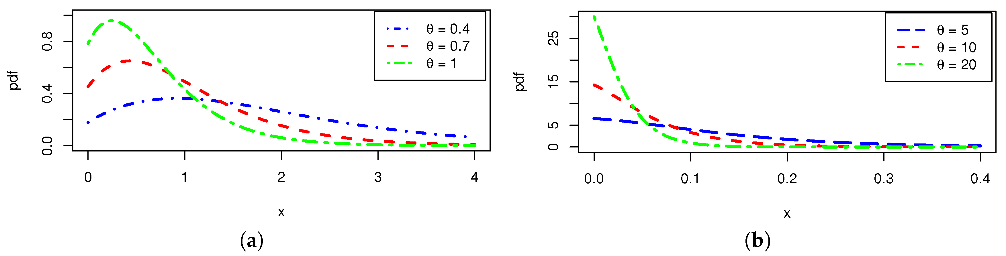
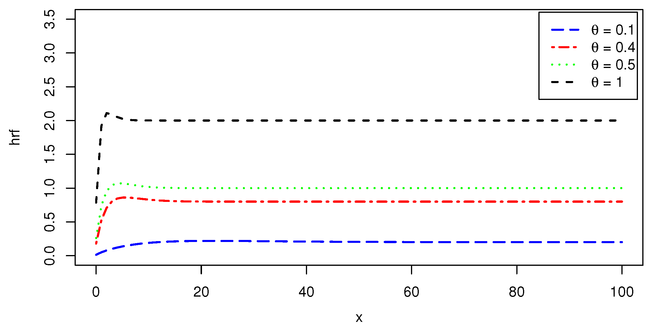
The immediate aim of the S-ML distribution is to use the S-G technique to enhance the effectiveness of the ML distribution on diverse data sets. In particular, thanks to the FOSO properties in Equations (3) and (6), it is a real and attractive alternative to the Lindley and ML distributions. Further exploration in the following research will reveal deeper motives. To summarise, the S-ML model’s utility and adaptability make it particularly appealing to fit data from various fields. Remarkably, the characterized pdf shows a variety of curve shapes, some of which have only one mode, are decreasing, and are asymmetrical to the right. In comparison to the pdf of the ML distribution, when it is unimodal, the pdf of the S-ML distribution has a more rounded peak, meaning that it is better adapted to fit a data histogram presenting a high kurtosis level. Furthermore, the S-ML distribution exhibits a non-monotonic hrf which is “increasing-reverse bathtub-constant” shaped. The hrf of the ML distribution has this feature as well. As with other competent models, the accuracy of the fits is persistent in the case of the S-ML model due to their characteristics. The claim is demonstrated by examining two published real-world data sets, primarily from engineering and climate data, against twelve competent models.

We prepare the rest of the paper in the following manner. The concept, quality, and key aspects of the S-ML distribution are covered in Section 2. A moment analysis is conducted in Section 3. The maximum likelihood estimation of the parameter $\theta$ is explained in Section 4. A simulation study is presented in Section 5. Section 6 assesses the proposed model’s applicability to real-world data. Finally, in Section 7, the conclusions are provided.

2. The S-ML Distribution

The mathematical foundation for the S-ML distribution is first presented.

2.1. Functional Analysis

To begin, we perform a functional analysis of the S-ML distribution. By substituting Equations (4) and (5) in Equations (1) and (2), respectively, we derive the major functions of the S-ML distribution; the cdf and pdf are given as follows

$$\begin{array}{cc}\hfill F_{S-ML}(x;\theta )& =\left\{\begin{array}{cc}cos\left[\frac{\pi }{2}\left(1+e^{-\theta x}\frac{x\theta }{1+\theta }\right)e^{-\theta x}\right],\hfill & \mathrm{if}x>0\hfill \\ 0,\hfill & \mathrm{if}x\le 0\hfill \end{array}\right.\hfill \end{array}$$

and

$$\begin{array}{cc}\hfill f_{S-ML}(x;\theta )& =\left\{\begin{array}{cc}\frac{\pi }{2}\frac{\theta }{1+\theta }{e}^{-2\theta x}\left[\left(1+\theta \right)e^{\theta x}+2x\theta -1\right]sin\left[\frac{\pi }{2}\left(1+e^{-\theta x}\frac{x\theta }{1+\theta }\right)e^{-\theta x}\right],\hfill & \mathrm{if}x>0\hfill \\ 0,\hfill & \mathrm{if}x\le 0\hfill \end{array}\right.,\hfill \end{array}$$

(7)

with $\theta >0$. As a primary result mentioned in the introduction section, the following FOSO property holds: $G_{ML}(x;\theta )\le F_{S-ML}(x;\theta )$ for any $x\in \mathbb{R}$, making an immediate difference between the ML and S-ML modeling from the cdf viewpoint. Differences can also be observed on the respective pdfs, as discussed below. Naturally, variant forms of $f_{S-ML}(x;\theta )$ can be obtained by changing the value of $\theta$. Due to the relative complexity of this function in the analytical sense, we propose a graphical study for shape analysis. The more representative shapes of this pdf are shown in Figure 1.

We can observe from Figure 1, that, for smaller values of $\theta$, the plot of $f_{S-ML}(x;\theta )$ is unimodal, and for larger values of $\theta$, the plot of $f_{S-ML}(x;\theta )$ is decreasing. As a result, the S-ML distribution is suitable for modeling a vast majority of lifetime phenomena. Compared to the parent ML distribution, the following observations are made: When it is unimodal, we observe that the pdf of the S-ML distribution has a more rounded peak, meaning that it is better adapted to fit a data histogram presenting a high kurtosis level. In other words, the S-ML model is more able to analyze data of a leptokurtic nature.

2.2. Reliability Analysis

We complete the previous functional analysis by studying the complementary reliability functions, such as the survival function (sf), hrf (for hazard rate function), reversed hrf (rhrf), second rate of failure (srf), and the cumulative hrf (chrf) of the S-ML distribution. In a broader sense, the sf measures the probability that the life of an item will survive beyond any specified time. Mathematically, the sf of the S-ML distribution is given by

$$\begin{array}{cc}\hfill S_{S-ML}(x;\theta )& =1-F_{S-ML}\left(x;\theta \right)=\left\{\begin{array}{cc}1-cos\left[\frac{\pi }{2}\left(1+e^{-\theta x}\frac{x\theta }{1+\theta }\right)e^{-\theta x}\right],\hfill & \mathrm{if}x>0\hfill \\ 1,\hfill & \mathrm{if}x\le 0\hfill \end{array}\right..\hfill \end{array}$$

The hrf measures the likelihood of an item deteriorating or expiring depending on its lifetime. As a direct consequence, it is critical in the classification of survival distributions. The hrf of the S-ML distribution is specified by

$$\begin{array}{cc}\hfill h_{S-ML}(x;\theta )& =\frac{f_{S-ML}(x;\theta )}{S_{S-ML}(x;\theta )}\hfill \\ & =\left\{\begin{array}{cc}\frac{\pi }{2}\frac{\theta }{1+\theta }{e}^{-2\theta x}\left[\left(1+\theta \right)e^{\theta x}+2x\theta -1\right]cot\left[\frac{\pi }{4}\left(1+e^{-\theta x}\frac{x\theta }{1+\theta }\right)e^{-\theta x}\right],\hfill & \mathrm{if}x>0\hfill \\ 0,\hfill & \mathrm{if}x\le 0\hfill \end{array}\right..\hfill \end{array}$$

Further, Figure 2 displays the shapes of this hrf for various values of $\theta$.

Figure 2 emphasizes that the hrf of the S-ML distribution has “increasing-reverse bathtub-constant” shapes, which is also possessed by the hrf of the ML distribution. This makes a solid difference between the Lindley and exponential distributions. It is also a desirable property for modelling purposes.

The rhrf is the ratio between the pdf to its cdf and it plays a role in analyzing censored data. Analytically, it corresponds to

$$\begin{array}{cc}\hfill r_{S-ML}(x;\theta )& =\left\{\begin{array}{cc}\frac{\pi }{2}\frac{\theta }{1+\theta }{e}^{-2\theta x}\left[\left(1+\theta \right)e^{\theta x}+2x\theta -1\right]tan\left[\frac{\pi }{2}\left(1+e^{-\theta x}\frac{x\theta }{1+\theta }\right)e^{-\theta x}\right],\hfill & \mathrm{if}x>0\hfill \\ 0,\hfill & \mathrm{if}x\le 0\hfill \end{array}\right..\hfill \end{array}$$

The srf is the logarithmic ratio of the sf at time x and $x+1$, and it is given by

$$\begin{array}{cc}\hfill r_{S-ML}^{*}(x;\theta )& =\left\{\begin{array}{cc}ln\left(\frac{1-cos\left[(\pi /2)\left(1+e^{-\theta x}x\theta /\left(1+\theta \right)\right)e^{-\theta x}\right]}{1-cos\left[(\pi /2)\left(1+e^{-\theta (x+1)}(x+1)\theta /(1+\theta )\right)e^{-\theta \left(x+1\right)}\right]}\right),\hfill & \mathrm{if}x>0\hfill \\ 0,\hfill & \mathrm{if}x\le 0\hfill \end{array}\right..\hfill \end{array}$$

The chrf is the negative logarithm of sf and is given by

$$\begin{array}{cc}\hfill H_{S-ML}(x;\theta )& =\left\{\begin{array}{cc}-ln\left(1-cos\left[\frac{\pi }{2}\left(1+e^{-\theta x}\frac{x\theta }{1+\theta }\right)e^{-\theta x}\right]\right),\hfill & \mathrm{if}x>0\hfill \\ 0,\hfill & \mathrm{if}x\le 0\hfill \end{array}\right..\hfill \end{array}$$

With these functions, we conclude different reliability analysis in regard with the S-ML distribution.

3. Moment Analysis

For any lifetime distribution, a moment analysis is necessary to handle numerically its modeling capacities, identifying the behavior of various central and dispersion moment parameters, as well as moment skewness and kurtosis coefficients.

As a first notion, for any positive integer $r\ge 1$, and a random variable X with the S-ML distribution, the r-th moment of X exists. It can be expressed as

$$\begin{array}{cc}\hfill \mathrm{mom}\left(r\right)& =\mathbb{E}\left(X^r\right)={\int }_0^{+\infty }{x}^r{f}_{S-ML}(x;\theta )dx\hfill \\ \hfill & =\frac{\pi }{2}\frac{\theta }{1+\theta }{\int }_0^{+\infty }{x}^r{e}^{-2\theta x}\left[\left(1+\theta \right)e^{\theta x}+2x\theta -1\right]sin\left[\frac{\pi }{2}\left(1+e^{-\theta x}\frac{x\theta }{1+\theta }\right)e^{-\theta x}\right]dx.\hfill \end{array}$$

(8)

Integral developments in the classical sense are limited. Computer software, on the other hand, can be used to quantitatively evaluate it for a given $\theta$.

We propose a series development of $\mathrm{mom}\left(r\right)$ in the next result, which can be used for computational purposes in a less opaq method than a “ready to use but black box” computer program.

Proposition 1.

The r-th moment of X can be expanded as

$$\begin{array}{cc}\hfill \mathrm{mom}\left(r\right)& =\frac{r}{{\theta }^r}\sum _{k=1}^{+\infty }\sum _{\ell =0}^{2k}\left(\genfrac{}{}{0pt}{}{2k}{\ell }\right)\frac{{(-1)}^{k+1}}{\left(2k\right)!}{\left(\frac{\pi }{2}\right)}^{2k}{(1+\theta )}^{-\ell }\frac{(\ell +r-1)!}{{(\ell +2k)}^{r+\ell }}.\hfill \end{array}$$

Proof. 

For the proof, we do not directly use the integral expression of $\mathrm{mom}\left(r\right)$ as described in (8). An integration by part gives

$$\begin{array}{cc}\hfill \mathrm{mom}\left(r\right)& ={\int }_0^{+\infty }{x}^r{f}_{S-ML}(x;\theta )dx=r{\int }_0^{+\infty }{x}^{r-1}{S}_{S-ML}(x;\theta )dx.\hfill \end{array}$$

Now, by utilizing the series expansion of the cosine function and the classical binomial formula, we obtain

$$\begin{array}{cc}\hfill S_{S-ML}(x;\theta )& =1-\sum _{k=0}^{+\infty }\frac{{(-1)}^k}{\left(2k\right)!}{\left(\frac{\pi }{2}\right)}^{2k}{\left(1+e^{-\theta x}\frac{x\theta }{1+\theta }\right)}^{2k}{e}^{-2k\theta x}\hfill \\ \hfill & =\sum _{k=1}^{+\infty }\frac{{(-1)}^{k+1}}{\left(2k\right)!}{\left(\frac{\pi }{2}\right)}^{2k}{\left(1+e^{-\theta x}\frac{x\theta }{1+\theta }\right)}^{2k}{e}^{-2k\theta x}\hfill \\ \hfill & =\sum _{k=1}^{+\infty }\sum _{\ell =0}^{2k}\left(\genfrac{}{}{0pt}{}{2k}{\ell }\right)\frac{{(-1)}^{k+1}}{\left(2k\right)!}{\left(\frac{\pi }{2}\right)}^{2k}{\left(\frac{\theta }{1+\theta }\right)}^{\ell }{x}^{\ell }{e}^{-(\ell +2k)\theta x}.\hfill \end{array}$$

(9)

Hence, after some developments including the change of variable $y=(\ell +2k)\theta x$ (so that $dx=[1/((\ell +2k)\theta \left)\right]dy$), and the calculus of gamma-type integral, we get

$$\begin{array}{cc}\hfill \mathrm{mom}\left(r\right)& =r{\int }_0^{+\infty }{x}^{r-1}\left[\sum _{k=1}^{+\infty }\sum _{\ell =0}^{2k}\left(\genfrac{}{}{0pt}{}{2k}{\ell }\right)\frac{{(-1)}^{k+1}}{\left(2k\right)!}{\left(\frac{\pi }{2}\right)}^{2k}{\left(\frac{\theta }{1+\theta }\right)}^{\ell }{x}^{\ell }{e}^{-(\ell +2k)\theta x}\right]dx\hfill \\ \hfill & =r\sum _{k=1}^{+\infty }\sum _{\ell =0}^{2k}\left(\genfrac{}{}{0pt}{}{2k}{\ell }\right)\frac{{(-1)}^{k+1}}{\left(2k\right)!}{\left(\frac{\pi }{2}\right)}^{2k}{\left(\frac{\theta }{1+\theta }\right)}^{\ell }{\int }_0^{+\infty }{x}^{r+\ell -1}{e}^{-(\ell +2k)\theta x}dx\hfill \\ \hfill & =\frac{r}{{\theta }^r}\sum _{k=1}^{+\infty }\sum _{\ell =0}^{2k}\left(\genfrac{}{}{0pt}{}{2k}{\ell }\right)\frac{{(-1)}^{k+1}}{\left(2k\right)!}{\left(\frac{\pi }{2}\right)}^{2k}{(1+\theta )}^{-\ell }\frac{(\ell +r-1)!}{{(\ell +2k)}^{r+\ell }}.\hfill \end{array}$$

Proposition 1 is proved. □

Then, based on Proposition 1, the following finite sum approximation remains acceptable:

$$\begin{array}{cc}\hfill \mathrm{mom}\left(r\right)& \approx \frac{r}{{\theta }^r}\sum _{k=1}^U\sum _{\ell =0}^{2k}\left(\genfrac{}{}{0pt}{}{2k}{\ell }\right)\frac{{(-1)}^{k+1}}{\left(2k\right)!}{\left(\frac{\pi }{2}\right)}^{2k}{(1+\theta )}^{-\ell }\frac{(\ell +r-1)!}{{(\ell +2k)}^{r+\ell }},\hfill \end{array}$$

where U represents any large integer.

From the above moment formulas, we can easily derive the mean, variance, moment skewness coefficient and moment kurtosis coefficient; the mean is given by $\mathrm{mom}\left(1\right)$, the variance is obtained as $\mathbb{V}\left(X\right)=\mathbb{E}\left({(X-\mathrm{mom}\left(1\right))}^2\right)$, the moment skewness coefficient can be derived as $\mathrm{MS}=\mathbb{E}\left({(X-\mathrm{mom}\left(1\right))}^3\right)/\mathbb{V}{\left(X\right)}^{3/2}$ and the moment kurtosis coefficient can be derived as $\mathrm{MK}=\mathbb{E}\left({(X-\mathrm{mom}\left(1\right))}^4\right)/\mathbb{V}{\left(X\right)}^2$.

Table 1. Values of various moment measures of the S-ML distribution.

$\mathit{\theta }$	mom(1)	$\mathbb{V}\left(\mathit{X}\right)$	MS	MK
0.5	1.448465	1.210367	1.449555	6.374828
1.0	0.6803329	0.3003946	1.520729	6.633623
1.5	0.4363871	0.1322356	1.573212	6.842306
2.0	0.318833	0.07375445	1.611987	7.005059
2.5	0.2502845	0.04687065	1.64148	7.133455
3.0	0.2056052	0.03235949	1.664569	7.236649

gives a glimpse of these values for different values of $\theta$.

From Table 1, we can observe that, as the value of the parameter $\theta$ of the S-ML distribution increases, all the considered measures increase. Furthermore, since $\mathrm{MS}>0$, it is clear that the S-ML distribution is mainly right-skewed, and since $\mathrm{MK}>3$, it is mainly leptokurtic.

We can complete the previous moment results by investigating the incomplete moments. To begin, let $r\ge 1$ be an integer, $t\ge 0$, and X be a random variable with the S-ML distribution. Based on this variable, we define its incomplete version by $Y\left(t\right)=X$ if $X\le t$ and $Y\left(t\right)=0$ if $X>t$. Then, the r-th incomplete moment of X given at t exists, and it is defined by

$$\begin{array}{cc}\hfill \mathrm{mom}(r,t)& =\mathbb{E}\left(Y{\left(t\right)}^r\right)={\int }_0^t{x}^r{f}_{S-ML}(x;\theta )dx.\hfill \end{array}$$

It is involved in developments of important probabilistic objects, such as mean deviations, income curves, etc. More basically, it can be viewed as a truncated version of the standard r-moment. We may refer to [15] in this regard.

In the next results, we present a series expansion of $\mathrm{mom}(r,t)$, which can be used for approximation purposes.

Proposition 2.

The r-th incomplete moment of X given at t exists and can be expanded as

$$\begin{array}{cc}\hfill \mathrm{mom}(r,t)& =-t^r\left\{1-cos\left[\frac{\pi }{2}\left(1+e^{-\theta t}\frac{t\theta }{1+\theta }\right)e^{-\theta t}\right]\right\}\hfill \\ \hfill & +\frac{r}{{\theta }^r}\sum _{k=1}^{+\infty }\sum _{\ell =0}^{2k}\left(\genfrac{}{}{0pt}{}{2k}{\ell }\right)\frac{{(-1)}^{k+1}}{\left(2k\right)!}{\left(\frac{\pi }{2}\right)}^{2k}{(1+\theta )}^{-\ell }\frac{1}{{(\ell +2k)}^{r+\ell }}\gamma (r+\ell ,(\ell +2k)\theta t),\hfill \end{array}$$

where $\gamma (a,t)$ denotes the incomplete gamma function defined by $\gamma (a,t)={\int }_0^t{x}^{a-1}{e}^{-x}dx$, where $a>0$ and $t\ge 0$.

Proof. 

The proof follows the lines of the one of Proposition 1. An integration by part gives

$$\begin{array}{cc}\hfill \mathrm{mom}(r,t)& ={\int }_0^t{x}^r{f}_{S-ML}(x;\theta )dx=-t^r{S}_{S-ML}(t;\theta )+r{\int }_0^t{x}^{r-1}{S}_{S-ML}(x;\theta )dx.\hfill \end{array}$$

It follows from the series expansion in Equation (9) and the change of variable $y=(\ell +2k)\theta x$ that

$$\begin{array}{cc}\hfill {\int }_0^t{x}^{r-1}{S}_{S-ML}(x;\theta )dx& =\sum _{k=1}^{+\infty }\sum _{\ell =0}^{2k}\left(\genfrac{}{}{0pt}{}{2k}{\ell }\right)\frac{{(-1)}^{k+1}}{\left(2k\right)!}{\left(\frac{\pi }{2}\right)}^{2k}{\left(\frac{\theta }{1+\theta }\right)}^{\ell }{\int }_0^t{x}^{r+\ell -1}{e}^{-(\ell +2k)\theta x}dx\hfill \\ \hfill & =\frac{1}{{\theta }^r}\sum _{k=1}^{+\infty }\sum _{\ell =0}^{2k}\left(\genfrac{}{}{0pt}{}{2k}{\ell }\right)\frac{{(-1)}^{k+1}}{\left(2k\right)!}{\left(\frac{\pi }{2}\right)}^{2k}{(1+\theta )}^{-\ell }\frac{1}{{(\ell +2k)}^{r+\ell }}\gamma (r+\ell ,(\ell +2k)\theta t).\hfill \end{array}$$

Therefore

$$\begin{array}{cc}\hfill \mathrm{mom}(r,t)& =-t^r\left\{1-cos\left[\frac{\pi }{2}\left(1+e^{-\theta t}\frac{t\theta }{1+\theta }\right)e^{-\theta t}\right]\right\}\hfill \\ \hfill & +\frac{r}{{\theta }^r}\sum _{k=1}^{+\infty }\sum _{\ell =0}^{2k}\left(\genfrac{}{}{0pt}{}{2k}{\ell }\right)\frac{{(-1)}^{k+1}}{\left(2k\right)!}{\left(\frac{\pi }{2}\right)}^{2k}{(1+\theta )}^{-\ell }\frac{1}{{(\ell +2k)}^{r+\ell }}\gamma (r+\ell ,(\ell +2k)\theta t).\hfill \end{array}$$

This concludes the proof of Proposition 2. □

In some sense, Proposition 2 generalizes Proposition 1; by taking $t\to +\infty$, Proposition 2 becomes Proposition 1.

The rest of the study is devoted to the applicability of the S-ML model, illustrated with concrete examples of data analysis.

4. Inferential Analysis

The inference of the S-ML model is covered in this section. The parameter $\theta$ is supposed to be unknown. In order to estimate it, the maximum likelihood estimation method is employed. We adopt the methodology as described in a broader context, as seen in [16].

Thus, the next is a mathematical representation of this methodology in the setting of the S-ML distribution. First, let n be a positive integer and $x_1,x_2,\dots ,x_n$ be observations drawn from a random variable X following the S-ML distribution. Then, the corresponding likelihood function and log-likelihood function are as follows

$$\begin{array}{cc}\hfill L& =\prod _{i=1}^n{f}_{S-ML}(x_i;\theta )={\left(\frac{\pi }{2}\right)}^n{\left(\frac{\theta }{1+\theta }\right)}^n{e}^{-2\theta {\sum }_{i=1}^n{x}_i}\prod _{i=1}^n\left[\left(1+\theta \right)e^{\theta x_i}+2x_i\theta -1\right]\hfill \\ \hfill & \times \prod _{i=1}^{n}sin\left[\frac{\pi }{2}\left(1+e^{-\theta x_i}\frac{x_i\theta }{1+\theta }\right)e^{-\theta x_i}\right],\hfill \end{array}$$

and

$$\begin{array}{cc}\hfill lnL& =nln\pi -nln2+nln\theta -nln\left(1+\theta \right)-2\theta \sum _{i=1}^n{x}_i\hfill \\ \hfill & +\sum _{i=1}^{n}ln\left[\left(1+\theta \right)e^{\theta x_i}+2x_i\theta -1\right]+\sum _{i=1}^{n}ln\left\{sin\left[\frac{\pi }{2}\left(1+e^{-\theta x_i}\frac{x_i\theta }{1+\theta }\right)e^{-\theta x_i}\right]\right\},\hfill \end{array}$$

respectively. The maximum likelihood estimate (MLE) of $\theta$ can be defined via the following argmax definition:

$$\begin{array}{c}\hfill \widehat{\theta }=argmax\underset{\theta >0}{ln}L.\end{array}$$

(10)

This estimate can be formalized through the solution of the non-linear equations expressed as $dlnL/d\theta =0$, where

$$\begin{array}{cc}\hfill \frac{d}{d\theta }lnL& =\frac{n}{\theta }-\frac{n}{1+\theta }-2\sum _{i=1}^n{x}_i+\sum _{i=1}^n\left[\frac{e^{\theta x_i}\left(\theta x_i+x_i+1\right)+2x_i}{(1+\theta )e^{\theta x_i}+2x_i\theta -1}\right]+\hfill \\ \hfill & \sum _{i=1}^n\left[\frac{\pi }{2}{e}^{-\theta x_i}\left(-\frac{\theta x_i^2{e}^{-\theta x_i}}{\theta +1}+\frac{x_i{e}^{-\theta x_i}}{\theta +1}-\frac{\theta x_i{e}^{-\theta x_i}}{{\left(\theta +1\right)}^2}\right)-\frac{\pi }{2}{x}_i{e}^{-\theta x_i}\left(1+\frac{\theta x_i{e}^{-\theta x_i}}{\theta +1}\right)\right]\hfill \\ \hfill & \times cot\left[\frac{\pi }{2}\left(1+e^{-\theta x_i}\frac{x_i\theta }{1+\theta }\right)e^{-\theta x_i}\right].\hfill \end{array}$$

There is no analytical solution for this equation, but $\widehat{\theta }$ can be determined at least numerically with any statistical software such as the R software (see [17]). Based on $\widehat{\theta }$, the estimated pdf (epdf) of the S-ML model is given by $f_{S-ML}(x;\widehat{\theta })$ and the estimated cdf (ecdf) of the S-ML model is given by $F_{S-ML}(x;\widehat{\theta })$.

Let $I\left(\theta \right)=-E[d^{2}ln\left[f_{S-ML}(X;\theta )\right]/d{\theta }^2]$ be the expected Fisher information matrix. Then, the estimated standard error (SE) of $\theta$ is achieved by considering the value of the diagonal component of $I{\left(\widehat{\theta }\right)}^{-1}$ raised to half.

5. Simulation Study

In the framework of the S-ML model, a simulation study is carried out to study the performance of $\widehat{\theta }$ given as Equation (10) in terms of their bias (bias) and mean squared error (MSE). The simulated procedure can be described as follows:

We generate samples of sizes $n=$ 20, 50, 100, 200, 500, 1000 from the S-ML distribution with $\theta =(1.25,1.50,2.00,2.50)$. For each sample, the MLE $\widehat{\theta }$ is calculated. Here, 1000 such repetitions are made to calculate the standard mean MLE (MMLE), bias and MSE of these estimates using the formula:

$$\begin{array}{cc}\hfill \mathrm{MMLE}\left(\widehat{\theta }\right)& =\frac{1}{1000}\sum _{i=1}^{1000}{\widehat{\theta }}_i,{\mathrm{Bias}}_{\theta }\left(\widehat{\theta }\right)=\frac{1}{1000}\sum _{i=1}^{1000}({\widehat{\theta }}_i-\theta )\hfill \end{array}$$

and

$$\begin{array}{cc}\hfill {\mathrm{MSE}}_{\theta }\left(\widehat{\theta }\right)& =\frac{1}{1000}\sum _{i=1}^{1000}{({\widehat{\theta }}_i-\theta )}^2,\hfill \end{array}$$

respectively, where ${\widehat{\theta }}_i$ is the estimate of $\theta$ for each iteration in the simulation study; i is from 1 to 1000. The results of the study are reported in

Table 2. Outcome of the simulation study.

θ	n	$\widehat{\mathit{\theta }}$
		Bias	MSE
1.25	20	0.040548	0.052057
	50	0.017112	0.0194051
	100	0.007862	0.009083
	200	0.005018	0.0045803
	500	0.002377	0.001814
	1000	0.001318	0.000915
1.50	20	0.51523	0.072304
	50	0.021153	0.028311
	100	0.008343	0.0125480
	200	0.005195	0.006043
	500	0.0027303	0.002816
	1000	0.001619	0.001239
2.00	20	0.060237	0.135020
	50	0.029170	0.052147
	100	0.012338	0.024522
	200	0.009004	0.012285
	500	0.001464	0.004796
	1000	0.003824	0.002366
2.50	20	0.106934	0.246197
	50	0.033415	0.083405
	100	0.023273	0.044903
	200	0.007408	0.019908
	500	0.007856	0.008118
	1000	0.001431	0.004158

.

From Table 2, it is observed that as sample size n increases,

• Bias decreases, which shows the accuracy of $\widehat{\theta }$;
• MSE decreases, which indicates the consistency (or preciseness) of $\widehat{\theta }$.

6. Applications of the S-ML Model

We use the S-ML model on two data sets based on the maximum likelihood method as introduced previously. The data differ in size, traits, and background, but they are all of current interest in their areas.

6.1. Method

We proceed as follows for each data set:

• The data are presented briefly, accompanied with their reference;
• A table that encapsulates the basic statistical measures of the data is provided;
• The goodness-of-fit measures of the models under consideration are evaluated and arranged in order of model performance in a table;
• The MLE(s) of the model parameters is(are) shown, as well as the relevant SEs, as supplementary work;
• It is concluded with a visual concept by presenting the histogram of the data and the epdf, as well as the empirical cdf plots and ecdf for the S-ML model exclusively in another graph.

The adequacy measures that are used for model fitting are provided here. Suppose $x_1,x_2,\dots ,x_n$ represent the data and $x_{\left(1\right)},x_{\left(2\right)},\dots ,x_{\left(n\right)}$ be their ordered values. As an initial step, we consider the Cramér von-Mises, Anderson Darling, and Kolmogorov–Smirnov statistics defined by

$$\begin{array}{c}\hfill A^{*}=-n-\sum _{i=1}^n\frac{2i-1}{n}\left[ln\left(F_{S-ML}(x_{\left(i\right)};\widehat{\theta })\right)+ln\left(S_{S-ML}(x_{(n+1-i)};\widehat{\theta })\right)\right],\end{array}$$

$$\begin{array}{c}\hfill W^{*}=\frac{1}{12n}+\sum _{i=1}^n{\left(F_{S-ML}(x_{\left(i\right)};\widehat{\theta })-\frac{2i-1}{2n}\right)}^2\end{array}$$

and

$$\begin{array}{c}\hfill D_n=\underset{i=1,2,\dots ,n}{max}\left(F_{S-ML}(x_{\left(i\right)};\widehat{\theta })-\frac{i-1}{n},\frac{i}{n}-F_{S-ML}(x_{\left(i\right)};\widehat{\theta })\right),\end{array}$$

respectively. The p-value of the Kolmogorov–Smirnov test linked to $D_n$ is also examined. Of course, the above definitions can be adapted to any other model than the S-ML model. The measures of adequacy are extensively employed to determine which model is best in terms of fitting the data set under study. The model having the least value for the $W^{*}$ or $A^{*}$, and the highest p-value, is considered to give the best fit that is in correspondence with the data.

Furthermore, we consider the following goodness-of-fit measures: Akaike information criterion (AIC) and Bayesian information criterion (BIC), given as follows

$$\begin{array}{c}\hfill \mathrm{AIC}=2k-2\mathrm{LL},\mathrm{BIC}=-2\mathrm{LL}+kln\left(n\right),\end{array}$$

respectively, where LL is the value of the log-likelihood function taken at $\widehat{\theta }$ and k, being the number of parameters of the model, here $k=1$ for the S-ML model. As it is widely understood, the model with the lowest value for AIC or BIC is selected as the greatest player of models that fits the data set compared to the other models. For more information on the usage and the underlying meaning of the measures $W^{*}$, $A^{*}$, $D_n$, AIC and BIC, we refer to [18].

In order to study the best fit of the S-ML model, we aim to compare it with some useful and competent models, which include the ML, Lindley, sine exponential and sine Lindley models listed in

Table 3. Competent models with the S-ML model.

Models	Abbreviations	Cdfs	References
Lindley	Lindley	$1-\left[1+\frac{x\theta }{1+\theta }\right]e^{-x\theta }$	[19]
sine exponential	S-Expo	$cos\left(\frac{\pi }{2}{e}^{-\theta x}\right)$	[2]
sine Lindley	S-Lindley	$cos\left[\frac{\pi }{2}\left(1+\frac{\theta x}{1+\theta }\right)e^{-\theta x}\right]$	[20]
modified Lindley	ML	$1-\left[1+e^{-\theta x}\frac{\theta x}{1+\theta }\right]e^{-\theta x}$	[11]
inverted modified Lindley	I-ML	$\left[1+\frac{\theta }{1+\theta }\frac{1}{x}{e}^{-\theta /x}\right]e^{-\theta /x}$	[21]
inverted Lindley	IL	$\left[1+\frac{\theta }{1+\theta }\frac{1}{x}\right]e^{-\theta /x}$	[22]
transmuted exponentiated inverse Rayleigh	TEIR	$e^{-\theta \alpha /x^2}\left[1+\lambda -\lambda e^{-\theta \alpha /x^2}\right]$	[23]
transmuted inverse Rayleigh	TIR	$e^{-\theta /x^2}\left[1+\lambda -\lambda e^{-\theta /x^2}\right]$	[24]
inverse Rayleigh	IR	$e^{-{\alpha /x}^2}$	[25]
Lomax	Lomax	$1-{\left[1+\frac{x}{\lambda }\right]}^{-\alpha }$	[26]
log normal	LNormal	$\varphi \left[\frac{lnx-\mu }{\sigma }\right]$	[27]
generalized beta type II	GB2	$\frac{\left|\alpha \right|}{{\beta }^{\alpha \theta }B(\theta ,\delta )}{\int }_0^x\frac{y^{\alpha \theta -1}}{{(1+{(y/\beta )}^{\alpha })}^{\theta +\delta }}dy$	[28]

. It is worth noting that models with three parameters are also considered. The aim is to prove that our model can be efficient enough to outperform more complex models in the literature.

6.2. Precipitation Data Set

The data set has thirty consecutive values of precipitation (in inches) in the month of March in Minneapolis, as provided by [29] and recently used by [30]. The data are: (0.77, 1.74, 0.81, 1.2, 1.95, 1.2, 0.47, 1.43, 3.37, 2.2, 3, 3.09, 1.51, 2.1, 0.52, 1.62, 1.31, 0.32, 0.59, 0.81, 2.81, 1.87, 1.18, 1.35, 4.75, 2.48, 0.96, 1.89, 0.9, 2.05). The descriptive statistical measures of these data are presented in

Table 4. Descriptive statistical measures for the precipitation data set.

Mean	Median	Variance	Skewness	Kurtosis	Min	Max
1.68	1.47	1	1.086682	4.206884	0.32	4.75

.

Based on the information in Table 4, the data are right-skewed and leptokurtic. The MLE, SE, and goodness-of-fit measures of the S-ML model and those of the other models for precipitation data set are given in

Table 5. MLEs, SEs, and goodness-of-fit measures for the precipitation data set with one parameter models.

Model	MLE (SE)	AIC	BIC	A*	W*	Dn	p-Value
S-ML	$\widehat{\theta }=0.44$ (0.0551)	82.9109	84.3121	0.6796	0.0972	0.1273	0.7153
ML	$\widehat{\theta }=0.6644$ (0.0974)	85.8898	87.291	1.1278	0.1723	0.1566	0.4532
Lindley	$\widehat{\theta }=0.9096$ (0.1247)	88.2874	89.6886	1.5908	0.2618	0.1882	0.2383
S-Expo	$\widehat{\theta }=0.3396$ (0.0576)	90.7932	92.1944	2.1771	0.3873	0.2202	0.1088
S-Lindley	$\widehat{\theta }=0.6091$ (0.0729)	85.6414	87.0426	1.1566	0.1817	0.1637	0.3966
I-ML	$\widehat{\theta }=1.247$ (0.1906)	89.7366	91.1378	1.3909	0.2170	0.1975	0.1925
IL	$\widehat{\theta }=1.5833$ (0.2268)	92.4423	1.8266	0.3040	0.1904	0.2279	0.0887
IR	$\widehat{\alpha }=0.8588$ (0.1568)	92.292	92.674	2.1822	0.43077	0.2396	0.06369

and

Table 6. MLEs, SEs, and goodness-of-fit measures for the precipitation data set with models having more than one parameter.

Model	MLE (SE)	AIC	BIC	A*	W*	Dn	p-Value
TEIR	$\widehat{\alpha }=1.1878$ (5.739)	90.2022	94.4058	1.1359553	0.2117553	0.1817501	0.2749038
	$\widehat{\lambda }=-0.67006$ (0.266)
	$\widehat{\theta }=0.6362$ (4.778)
TIR	$\widehat{\lambda }=0.0001$ (0.40171)	91.073	94.759	1.136	0.21177	0.1817	0.2748
	$\widehat{\theta }=0.8588$ (0.2136)
Lomax	$\widehat{\alpha }=58619.76$ (52.96)	94.9	97.8	2.5139	0.4539	0.2352	0.0724
	$\widehat{\lambda }=$ 98190 (96.69)
LNormal	$\widehat{\mu }=0.33737$ (0.11368)	81	83.8	0.19855	0.0311	0.0913	0.9640
	$\widehat{\sigma }=0.62263$ (0.08038)
GB2	$\widehat{\alpha }=580.4141$ (1593.1699)	84.1	89.7	7.43	1.58	0.445	0.0000138
	$\widehat{\beta }=0.8125$ (0.6469)
	$\widehat{\theta }=4.3731$ (6.6885)
	$\widehat{\delta }=520.2863$ (584.0752)

.

We can observe from Table 5 that the S-ML model has the lowest statistics with the highest p-value, implying that it delivers a better fit than the other models studied. Comparing the models in Table 6, we can see that the lognormal model gives a better fit, while the S-ML model takes the second place, but with less modeling complexity in terms of the number of parameters. Figure 3 depicts the epdf and ecdf plots of the S-ML model for the precipitation data set.

From Figure 3, it is obvious that the S-ML model captures the histogram’s overall pattern and illustrates the comparison of the cdf with the empirical cdf of the S-ML model. The suitable behaviour of the S-ML model is further confirmed by these graphs. Apart from the lognormal model, the S-ML model clearly fits better than the Lindley, ML, S-Expo and S-Lindley, and other models.

6.3. Time between Failure Data Set

This data set refers to the time between failures for repairable items. It was obtained from [31]. The data are: (1.43, 0.11, 0.71, 0.77, 2.63, 1.49, 3.46, 2.46, 0.59, 0.74, 1.23, 0.94, 4.36, 0.40, 1.74, 4.73, 2.23, 0.45, 0.70, 1.06, 1.46, 0.30, 1.82, 2.37, 0.63, 1.23, 1.24, 1.97, 1.86, 1.17). The descriptive statistical measures of these data are presented in

Table 7. Descriptive statistical measures for the failure time data set.

Mean	Median	Variance	Skewness	Kurtosis	Min	Max
1.542667	1.235000	1.127167	1.295462	4.319170	0.110000	4.730000

.

From Table 7, we can observe that the failure time data set is right-skewed and leptokurtic.

The MLE, SE, and goodness-of-fit measures of the S-ML model and those of the other models for the failure time data set are given in

Table 8. MLEs, SEs, and goodness-of-fit measures for the failure time data set with one parameter models.

Model	MLE (SE)	AIC	BIC	A*	W*	Dn	p-Value
S-ML	$\widehat{\theta }=0.47420\left(0.06039\right)$	82.3276	83.7288	0.22656158	0.02897235	0.07805138	0.99313719
ML	$\widehat{\theta }=0.7297\left(0.1082\right)$	83.5051	84.9063	0.4401	0.0650	0.1112	0.8514
Lindley	$\widehat{\theta }=0.9762\left(0.1345\right)$	85.0946	86.4958	0.7265	0.1138	0.1406	0.5929
S-Expo	$\widehat{\theta }=0.3662\left(0.0625\right)$	86.5547	87.9559	1.0582	0.17981	0.16722	0.3711
S-Lindley	$\widehat{\theta }=0.64690\left(0.0783\right)$	83.7386	85.1398	0.4599	0.0654	0.1139	0.8310
I-ML	$\widehat{\theta }=0.9222\left(0.1361\right)$	92.6416	94.0426	0.9582	0.1430	0.1394	0.6043
IL	$\widehat{\theta }=1.1603\left(0.1619\right)$	95.8658	97.2670	1.261	0.1904	0.1411	0.5879
IR	$\widehat{\alpha }=0.237\left(0.043\right)$	135.289	136.690	1.423	2.410	0.442	0.00001

and

Table 9. MLEs, SEs, and goodness-of-fit measures for the failure time data set with models having more than one parameter.

Model	MLE (SE)	AIC	BIC	A*	W*	Dn	p-Value
TEIR	$\widehat{\alpha }=0.022\left(0.065\right)$	122.99	127.19	8.373	1.47	0.37	0.000410
	$\widehat{\lambda }=-0.880\left(0.114\right)$
	$\widehat{\theta }=8.211\left(23.735\right)$
TIR	$\widehat{\lambda }=-0.880\left(0.114\right)$	120.990	123.792	8.369	1.471	0.3761	0.0004
	$\widehat{\theta }=0.185\left(0.035\right)$
Lomax	$\widehat{\alpha }=19793.12\left(81.02\right)$	90	92.8	1.33	0.232	0.184	0.259
	$\widehat{\lambda }=305\left(51.04\right))$
LNormal	$\widehat{\mu }=0.1597\left(0.1464\right)$	85.5	88.3	0.2577	0.0369	0.0987	0.9322
	$\widehat{\sigma }=0.801\left(0.1035\right)$
GB2	$\widehat{\alpha }=655.80\left(2342.40\right)$	87.2	92.8	7.53	1.64	0.042	0.00003
	$\widehat{\beta }=0.907\left(0.77\right)$
	$\widehat{\theta }=2.351\left(3.56\right)$
	$\widehat{\delta }=582.259\left(519.98\right)$

.

Table 8 and Table 9 show that, for the failure time data set, the S-ML model has the lowest statistics and the highest p-value, meaning that it provides a better match than the other models investigated.

Figure 4 depicts the epdf and ecdf plots of the S-ML model for the failure time data set.

From Figure 4, it is obvious that the S-ML model captures the histogram’s overall pattern and illustrates the comparison of the cdf with the empirical cdf of the S-ML model. The suitable behaviour of the S-ML model is further confirmed by these graphs.

7. Conclusions

The article’s major contribution is a flexible trigonometric extension of the well-known modified Lindley model that proposes a novel efficient statistical modelling technique. We employ the features of the sine generalized family of distributions in this regard, and develop the sine modified Lindley distribution. We have displayed a few of its more noteworthy attributes, with a focus on the shape properties of the corresponding probability density and hazard rate functions, as well as discussing moments. Simulation studies and applications demonstrate the utility of the model under consideration. In particular, we compared it to the primary current models derived from the Lindley, exponential and other models with one or more parameters, using two real-world data sets. As a result, the obtained findings are really satisfactory, demonstrating that the novel distribution has a wide range of applications that could be the subject of additional research in a variety of scientific fields.

References

1. Brito, C.R.; Rêgo, L.C.; Oliveira, W.R.; Gomes-Silva, F. Method for generating distributions and classes of probability distributions: The univariate case. Hacet. J. Math. Stat. 2019, 48, 897–930. [Google Scholar]
2. Kumar, D.; Singh, U.; Singh, S.K. A new distribution using sine function: Its application to bladder cancer patients data. J. Stat. Appl. Probab. 2015, 4, 417–427. [Google Scholar]
3. Souza, L. New Trigonometric Classes of Probabilistic Distributions. Ph.D. Thesis, Universidade Federal Rural de Pernambuco, Recife, Brazil, 2015. [Google Scholar]
4. Souza, L.; Junior, W.R.O.; de Brito, C.C.R.; Chesneau, C.; Ferreira, T.A.E.; Soares, L. On the Sin-G class of distributions: Theory, model and application. J. Math. Model 2019, 7, 357–379. [Google Scholar] [CrossRef]
5. Nelson, W. Applied Life Data Analysis; John Wiley & Sons: New York, NY, USA, 1982. [Google Scholar]
6. Nagarjuna, V.B.V.; Vardhan, R.V.; Chesneau, C. On the Accuracy of the Sine Power Lomax Model for Data Fitting. Modelling 2021, 2, 5. [Google Scholar] [CrossRef]
7. Souza, L.; Junior, W.R.O.; de Brito, C.C.R.; Chesneau, C.; Ferreira, T.A.E.; Soares, L. General properties for the Cos-G class of distributions with applications. Eurasian Bull. Math. 2019, 2, 63–79. [Google Scholar]
8. Chesneau, C.; Jamal, F. The sine Kumaraswamy-G family of distributions. J. Math. Ext. 2021, 15, 1–33. [Google Scholar]
9. Al-Babtain, A.A.; Elbatal, I.; Chesneau, C.; Elgarhy, M. Sine Topp-Leone-G family of distributions: Theory and applications. Open Phys. 2020, 18, 574–593. [Google Scholar] [CrossRef]
10. Souza, L.; Junior, W.R.O.; de Brito, C.C.R.; Chesneau, C.; Ferreira, T.A.E.; Fernandes, L.R. Tan-G class of trigonometric distributions and its applications. Cubo 2021, 23, 1–20. [Google Scholar] [CrossRef]
11. Chesneau, C.; Tomy, L.; Gillariose, J. A new modified Lindley distribution with properties and applications. J. Stat. Manag. Syst. 2021. [Google Scholar] [CrossRef]
12. Chesneau, C.; Tomy, L.; G, V. The Poisson-modified Lindley distribution. Appl. Math. E Notes. in press.
13. Chesneau, C.; Tomy, L.; Jose, M. Wrapped modified Lindley distribution. J. Stat. Manag. Syst. 2021. [Google Scholar] [CrossRef]
14. Tomy, L.; G, V.; Chesneau, C. The discrete modified Lindley distribution. 2021; unpublished work. [Google Scholar]
15. Cordeiro, G.M.; Silva, R.B.; Nascimento, A.D.C. Recent Advances in Lifetime and Reliability Models; Bentham Books: Sharjah, United Arab Emirates, 2020. [Google Scholar] [CrossRef]
16. Casella, G.; Berger, R.L. Statistical Inference; Duxbury Advanced Series Thomson Learning: Pacific Grove, CA, USA, 2002. [Google Scholar]
17. R Development Core Team. R: A Language and Environment for Statistical Computing; R Foundation for Statistical Computing: Vienna, Austria, 2005. [Google Scholar]
18. Konishi, S.; Kitagawa, G. Information Criteria and Statistical Modeling; Springer: New York, NY, USA, 2007. [Google Scholar]
19. Lindley, D.V. Fiducial distributions and Bayes theorem. J. R. Stat. Soc. A 1958, 20, 102–107. [Google Scholar] [CrossRef]
20. Kumar, D.; Singh, U.; Singh, S.K.; Chaurasia, P.K. Statistical properties and application of a Lifetime model using sine function. Int. J. Creat. Res. Thoughts 2018, 6, 993–1002. [Google Scholar]
21. Chesneau, C.; Tomy, L.; Gillariose, J.; Jamal, F. The inverted modified Lindley distribution. J. Stat. Theory Pract. 2020, 14, 1–17. [Google Scholar] [CrossRef]
22. Sharma, V.; Singh, S.; Singh, U.; Agiwal, V. The inverse Lindley distribution: A stress-strength reliability model with applications to head and neck cancer data. J. Ind. Prod. Eng. 2015, 32, 162–173. [Google Scholar] [CrossRef]
23. Haq, M.A. Transmuted exponentiated inverse Rayleigh distribution. J. Stat. Appl. Prob. 2016, 5, 337–343. [Google Scholar] [CrossRef]
24. Ahmad, A.; Ahmad, S.; Ahmed, A. Transmuted Inverse Rayleigh Distribution: A Generalization of the Inverse Rayleigh Distribution. Math. Theory Model. 2014, 4, 90–98. [Google Scholar]
25. Voda, V.G. On the inverse Rayleigh distributed random variable. Rep. Statist. App. Res. 1972, 19, 13–21. [Google Scholar]
26. Lomax, K.S. Business Failures, Another example of the analysis of failure data. J. Am. Stat. Assosciation 1954, 49, 847–852. [Google Scholar] [CrossRef]
27. Aitchinson, J.; Brown, J.A.C. The Lognormal Distribution; Cambridge University Press: Cambridge, UK, 1957. [Google Scholar]
28. Kalbfleisch, J.D.; Prentice, R.L. The Statistical Analysis of Failure Time Data; Wiley: New York, NY, USA, 1980. [Google Scholar]
29. Hinkley, D. On quick choice of power transformation. Appl. Stat. 1977, 26, 67–69. [Google Scholar] [CrossRef]
30. Yusuf, A.; Mikail, B.B.; Aliyu, A.I.; Sulaiman, A.L. The Inverse Burr Negative Binomial Distribution with Application to Real Data. Stat. J. Theor. Appl. Stat. 2016, 5, 53–65. [Google Scholar] [CrossRef]
31. Murthy, D.P.; Xie, M.; Jiang, R. Weibull Models; Wiley: Hoboken, NJ, USA, 2004. [Google Scholar]
Figure 1. Plots of (a) unimodal shapes and (b) decreasing shapes for f S M L ( x ; θ ) .
Mca 26 00081 g001
Figure 2. Plots of h S M L ( x ; θ ) with selected values of θ .
Mca 26 00081 g002
Figure 3. Plots of the (a) epdf and (b) ecdf of the S-ML model for the precipitation data set.
Mca 26 00081 g003
Figure 4. Plots of the (a) epdf and (b) ecdf of the S-ML model for the failure time data set.
Mca 26 00081 g004