Using the Evolution Operator to Classify Evolution Algebras †


Abstract
1. Introduction
2. Preliminaries on Evolution Algebras
3. Evolution Algebras Whose Evolution Operator Is a Derivation
- If E is non-degenerate, then its dimension is even, and the structure matrix is a block diagonal matrix , wherefor some .
- If E is degenerate, the following algorithm to obtain all the structure matrices A of these algebras in dimension n is given.
- Step 1:
- Obtain all matrices of dimension , both degenerate and non-degenerate.
- Step 2:
- For each , impose conditionsand (2) on matrix .
3.1. The Algorithm
- If , then these conditions are fulfilled, since all of these indices are from the submatrix .
- If or , then these conditions are .

3.2. Computational and Complexity Study
- The auxiliary function has complexity , since the loop is executed n times.
- The definition of has complexity .
- The definition of has complexity , since the loop is executed times and, in each iteration, the auxiliary function is called.
3.3. Five-Dimensional Evolution Algebras
- For : We can assume that , since, if any of these constants is null, it would be treated as the following cases (if necessary, by a permutation of the basis). If we run the following code
 then we obtain , so we get the matrices of the form
- For : We can assume that . Running the algorithm, we obtain . That is, matrices of the form
- For : We can assume that . Running the algorithm, we get the matricesdepending on whether the constants b and c are null.
- For : We can assume that . Running the algorithm, we get , which corresponds to the matrices
- For : We can assume that a and b are not both null, the same as c and d. Running the algorithm, we obtain , so we get the matrices
- For : Running the algorithm, we obtain the matricesdepending on whether the constants are null.

3.4. Characterization in the Degenerate Case
- A)
- where
- D is a matrix of the form , for some r with and .
- O is the zero matrix.
- is a matrix whose only non-null elements are in the lower left submatrix, for some k with , and such that its columns fulfill that , , ⋯, .
- B)
- where
- is the zero matrix, for some .
- is the zero matrix.
- is the zero matrix.
- is a matrix.
- Case 1:
- is non-degenerate. Then, , for some . From condition (3), we obtain that , , ⋯, . Thus, matrix A is like in A).
- Case 2:
- is like (5). Let be the lower submatrix in .If is null, from condition (3), we obtain that , , ⋯, . Thus, A is like in A), being .In another case, we can assume that the submatrix of does not have any null rows, since, in this case, we could reorder the basis so that this non-null matrix would be of size and could be treated as one of size , in which that null row would no longer appear.Since no row is null, from Remark 1, we obtain that . Again, by condition (3), , , ⋯, . Thus, A is like in A).
- Case 3:
- is like (6). Let be the lower submatrix in . If is null, then A is trivially like in B).In another case, we can assume, as before, that, in the submatrix of , there is no null row. Then, by Remark 1, we obtain . Thus, A is like in B).
3.5. Six-Dimensional Evolution Algebras
4. Applications
5. Conclusions
- When the evolution operator is a derivation, it is easy to check that the equality holds for . An operator is said to be a derivation of ordern when it satisfies the above equality for n. It could be studied when the evolution operator is a derivation of orden n, for .
- When the evolution operator is a derivation, it is also easy to check that the equality holds for . An operator is said to be a n-derivation when it satisfies the above equality for n. It could be studied when the evolution operator is an n-derivation, for .
- Classify evolution algebras whose evolution operator satisfies other equalities. For example, the case in which the evolution operator is an endomorphism of algebras is analyzed in [21], that is, when . This case could be studied in depth.
- Transfer the results obtained to other branches of Mathematics that have direct connections with evolution algebras.
Author Contributions
Funding
Conflicts of Interest
References
- Tian, J.P. Evolution Algebra Theory. Ph.D. Thesis, University of California, Riverside, CA, USA, 2004. [Google Scholar]
- Tian, J.P. Evolution Algebras and Their Applications; Springer: Berlin, Germany, 2008. [Google Scholar]
- Tian, J.P.; Vojtechovsky, P. Mathematical concepts of evolution algebras in non-Mendelian genetics. Quasigr. Relat. Syst. 2006, 14, 111–122. [Google Scholar]
- Elduque, A.; Labra, A. Evolution algebras and graphs. J. Algebra Appl. 2015, 14, 1550103. [Google Scholar] [CrossRef]
- Núñez, J.; Rodríguez, M.L.; Villar, M.T. Certain particular families of graphicable algebras. Appl. Math. Comput. 2014, 246, 416–425. [Google Scholar] [CrossRef]
- Núñez, J.; Silvero, M.; Villar, M.T. Mathematical tools for the future: Graph Theory and graphicable algebras. Appl. Math. Comput. 2013, 219, 6113–6125. [Google Scholar] [CrossRef]
- Cadavid, P.; Rodiño, M.L.; Rodriguez, P.M. The connection between evolution algebras, random walks and graphs. J. Algebra Appl. 2018, 19, 2050023. [Google Scholar] [CrossRef]
- López, F.; Núñez, J.; Recacha, S.; Villar, M.T. Connecting Statistics, Probability, Algebra and Discrete Mathematics. arXiv 2021, arXiv:2104.02470. [Google Scholar]
- Wears, T.H. On algebraic solitons for geometric evolution equations on three-dimensional Lie groups. Tbilisi Math. J. 2016, 9, 2. [Google Scholar] [CrossRef][Green Version]
- Falcón, O.J.; Falcón, R.M.; Núñez, J. Classification of asexual diploid organisms by means of strongly isotopic evolution algebras defined over any field. J. Algebra. 2017, 472, 573–593. [Google Scholar] [CrossRef]
- Li, T.; Viglialoro, G. Boundedness for a nonlocal reaction chemotaxis model even in the attraction-dominated regime. Differ. Integral Equ. 2021, 34, 315–336. [Google Scholar]
- Viglialoro, G.; Woolley, T.E. Solvability of a Keller-Segel system with signal-dependent sensitivity and essentially sublinear production. Appl. Anal. 2020, 99, 2507–2525. [Google Scholar] [CrossRef]
- Ghasemi, M.; Infusino, M.; Kuhlmann, S.; Marshall, M. Moment problem for symmetric algebras of locally convex spaces. Integral Equ. Oper. Theory 2018, 90, 1–19. [Google Scholar] [CrossRef]
- Alsarayreh, A.; Qaralleh, I.; Ahmad, M.Z. Derivation of three-dimensional evolution algebra. JP J. Algebra Number Theory Appl. 2017, 39, 425–444. [Google Scholar] [CrossRef]
- Cadavid, P.; Rodiño, M.L.; Rodriguez, P.M. Characterization theorems for the spaces of derivations of evolution algebras associated with graphs. Linear Multilinear Algebra 2020, 68, 1340–1354. [Google Scholar] [CrossRef]
- Camacho, L.M.; Gómez, J.R.; Omirov, B.A.; Turdibaev, R.M. The derivations of some evolution algebras. Linear Multilinear Algebra 2013, 61, 309–322. [Google Scholar] [CrossRef]
- Mukhamedov, F.; Khakimov, O.; Omirov, B.; Qaralleh, I. Derivations and automorphisms of nilpotent evolution algebras with maximal nilindex. J. Algebra Appl. 2019, 18, 1950233. [Google Scholar] [CrossRef]
- Cabrera, Y.; Siles, M.; Velasco, M.V. Classification of three-dimensional evolution algebras. Linear Algebra Appl. 2017, 524, 68–108. [Google Scholar] [CrossRef]
- Houida, A.; Ural, B.; Isamiddin, R. On classification of two-dimensional evolution algebras and its applications. J. Phys. Conf. Ser. 2020, 1489. [Google Scholar] [CrossRef]
- Murodov, S.N. Classification of two-dimensional real evolution algebras and dynamics of some two-dimensional chains of evolution algebras. Uzbek. Mat. Zh. 2014, 2, 102–111. [Google Scholar]
- Fernández-Ternero, D.; Gómez-Sousa, V.M.; Núñez-Valdés, J. The evolution operator of evolution algebras. Linear Multilinear Algebra 2021. [Google Scholar] [CrossRef]
- Absalamov, A.T.; Rozikov, U.A. The dynamics of gonosomal evolution operators. J. Appl. Nonlinear Dyn. 2020, 9, 247–257. [Google Scholar] [CrossRef]
- Padmanabhan, T. Probing the Planck scale: The modification of the time evolution operator due to the quantum structure of spacetime. J. High Energy Phys. 2020, 11, 13. [Google Scholar] [CrossRef]
- Akararungruangkul, R.; Kaewman, S. Modified differential evolution algorithm solving the special case of location routing problem. Math. Comput. Appl. 2018, 23, 34. [Google Scholar] [CrossRef]
- Kaewman, S.; Srivarapongse, T.; Theeraviriya, C.; Jirasirilerd, G. Differential evolution algorithm for multilevel assignment problem: A case study in chicken transportation. Math. Comput. Appl. 2018, 23, 55. [Google Scholar] [CrossRef]
- Sriboonchandr, P.; Kriengkorakot, N.; Kriengkorakot, P. Improved differential evolution algorithm for flexible job shop scheduling problems. Math. Comput. Appl. 2019, 24, 80. [Google Scholar] [CrossRef]


| Input | Computing Time (s) | Input | Computing Time (s) |
|---|---|---|---|
| 0.0 | 4.047 | ||
| 0.031 | 7.516 | ||
| 0.094 | 12.641 | ||
| 0.203 | 19.625 | ||
| 0.406 | 29.313 | ||
| 0.688 | 41.016 | ||
| 1.875 | 55.797 |
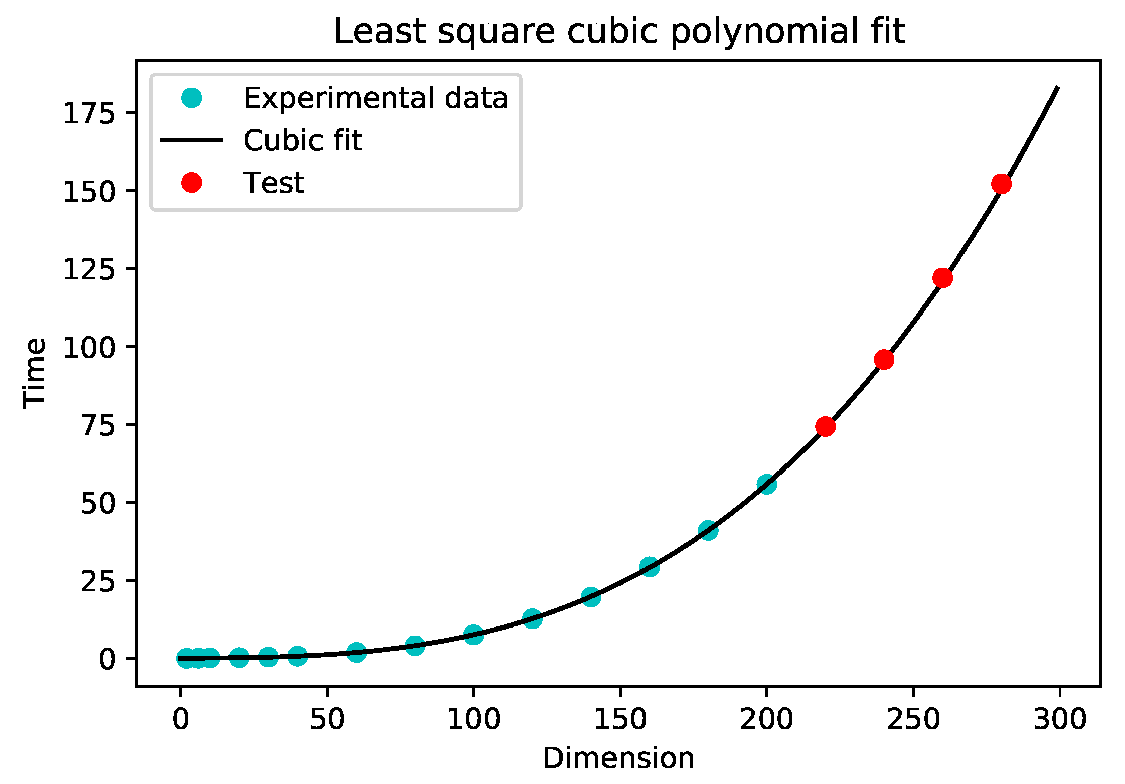
| Input | Computing Time (s) | Expected Time (s) |
|---|---|---|
| 74.297 | 73.882 | |
| 95.797 | 95.450 | |
| 121.969 | 120.867 | |
| 152.188 | 150.449 |
Publisher’s Note: MDPI stays neutral with regard to jurisdictional claims in published maps and institutional affiliations. |
© 2021 by the authors. Licensee MDPI, Basel, Switzerland. This article is an open access article distributed under the terms and conditions of the Creative Commons Attribution (CC BY) license (https://creativecommons.org/licenses/by/4.0/).
Share and Cite
Fernández-Ternero, D.; Gómez-Sousa, V.M.; Núñez-Valdés, J. Using the Evolution Operator to Classify Evolution Algebras. Math. Comput. Appl. 2021, 26, 57. https://doi.org/10.3390/mca26030057
Fernández-Ternero D, Gómez-Sousa VM, Núñez-Valdés J. Using the Evolution Operator to Classify Evolution Algebras. Mathematical and Computational Applications. 2021; 26(3):57. https://doi.org/10.3390/mca26030057
Chicago/Turabian StyleFernández-Ternero, Desamparados, Víctor M. Gómez-Sousa, and Juan Núñez-Valdés. 2021. "Using the Evolution Operator to Classify Evolution Algebras" Mathematical and Computational Applications 26, no. 3: 57. https://doi.org/10.3390/mca26030057
APA StyleFernández-Ternero, D., Gómez-Sousa, V. M., & Núñez-Valdés, J. (2021). Using the Evolution Operator to Classify Evolution Algebras. Mathematical and Computational Applications, 26(3), 57. https://doi.org/10.3390/mca26030057