Article

Some Aspects of Numerical Analysis for a Model Nonlinear Fractional Variable Order Equation

1
Institute of Cosmophysical Research and Radio Wave Propagation, Far Eastern Branch of the Russian Academy of Sciences, 684034 Kamchatskiy Kray, Russia
2
Faculty of Physics and Mathematics, Vitus Bering Kamchatka State University, 683032 Petropavlovsk-Kamchatskiy, Russia
*
Author to whom correspondence should be addressed.
Math. Comput. Appl. 2021, 26(3), 55; https://doi.org/10.3390/mca26030055
Submission received: 14 July 2021 / Revised: 26 July 2021 / Accepted: 28 July 2021 / Published: 29 July 2021
(This article belongs to the Section Natural Sciences)

Abstract

:
The article proposes a nonlocal explicit finite-difference scheme for the numerical solution of a nonlinear, ordinary differential equation with a derivative of a fractional variable order of the Gerasimov–Caputo type. The questions of approximation, convergence, and stability of this scheme are studied. It is shown that the nonlocal finite-difference scheme is conditionally stable and converges to the first order. Using the fractional Riccati equation as an example, the computational accuracy of the numerical method is analyzed. It is shown that with an increase in the nodes of the computational grid, the order of computational accuracy tends to unity, i.e., to the theoretical value of the order of accuracy.

1. Introduction

At present, fractional calculus is widely developed, which is discussed in detail in monographs [1,2,3,4,5], as well as in survey articles, for example [6].
Fractional calculus studies fractional derivatives and integrals, as well as their applications. It is thanks to the applications that fractional calculus is intensively used in physics [7,8], mechanics [9,10,11], biology [12,13], economics [14,15] and other sciences. We will not dwell here on the interpretation of the meaning of the fractional derivative. We refer the reader to other works, such as [16], for discussions on this problem.
In the 1990s, within the framework of fractional calculus, there appeared a direction devoted to fractional operators of variable order (FO-VO) [17]. This direction received a powerful impetus for development, which is associated with the emergence of various complex problems in physics, mechanics, biology, economics, and other sciences, which are well described by FO-VO. For example, it was shown in [12] that the kinetics of the reaction of proteins demonstrates relaxation mechanisms that are properly described by the temperature-dependent fractional-order operator. The survey article [18] described the development of fractional calculus as fractional operators of constant and variable orders, and considered analytical and numerical methods for their study.
Of great practical importance is the application of numerical methods of analysis to the solution of nonlinear equations with derivatives of fractional orders [19,20,21,22,23,24,25,26,27]. This is due to the fact that numerical methods provide a quantitative description of the parameters of the process under study. However, as a rule, questions arise here related to the stability and convergence of numerical methods. In this paper, we investigate these issues, using an explicit finite-difference scheme in order to find a numerical solution to a nonlinear equation with a fractional variable order derivative. This equation can be a model and describe various processes, for example, processes with saturation.
In the paper, the necessary concepts and definitions are first given; then, the formulation of the problem is revealed, the method of solution is given, the issues of approximation, stability and convergence of the scheme are considered, and specific examples are given.

2. Preliminary Information

Definition 1.
The Euler gamma function is determined according to the following integral:
Γ x = 0 e t t x 1 d t , x : x > 0 .
Remark 1.
It should be noted that the Euler gamma function is monotonically decreasing over the interval 0 < x < 1 .
Definition 2.
A continuous function f u , t C 0 , T satisfies the Lipschitz condition with a constant L in the variable u t C 0 , T :
f u 1 , t f u 2 , t < L u 1 u 2 ,
Definition 3.
The operator of the fractional variable order 0 < α t < 1 acts on a function u t C 0 , T :
0 t α t u t = 1 Γ 1 α t 0 t u ˙ σ d σ t σ α t ,
where Γ · is the Euler gamma function (1) and u ˙ t = d u d u d t d t will be called the derivative of a fractional variable order of the Gerasimov–Caputo type.
The properties of operator (3) can be found in [28].
Definition 4.
Equations containing derivatives of a fractional variable order of the Gerasimov–Caputo type (3) will be called fractional equations.
Remark 2.
In the case when operator (3) has a constant order, i.e., α does not depend on t, we obtain the Gerasimov–Caputo operator [29,30].

3. Problem Statement and Solution Method

Consider the following Cauchy problem for a nonlinear fractional equation:
0 t α t u t b t u t = f u , t , u 0 = u 0 ,
where u t C 0 , T is the solution function, t 0 , T is the time, T is the model time, u 0 is a given constant, 0 < b t is a continuous function, f u , t is a nonlinear function satisfying the Lipschitz condition (2) with a constant L in the variable u t , and the operator of a fractional variable order has view (1).
Remark 3.
The Cauchy problem (1) describes a wide class of dynamic processes with variable memory [11].
Due to the nonlinearity of the Cauchy problem (4), we will seek its solution using the numerical method of finite-difference schemes [31,32,33]. Consider a uniform mesh.
To do this, we divide the segment 0 , T into N equal parts—grid nodes with a step τ = T T N N . We assume that the function u t satisfies the necessary smoothness for constructing a finite-difference scheme, i.e., u t C 2 0 , T . Then, the solution function u t goes over to the grid solution function u t k or u k , where t k = k τ , k = 0 , , N 1 .
An approximation of the derivative of a fractional variable order of the Gerasimov–Caputo type in Equation (4) can be written as follows:
0 t α t u t = 1 Γ 1 α t 0 t u ˙ σ d σ t σ α t 1 Γ 1 α k j = 0 k 1 j τ j + 1 τ u ˙ σ d σ t k + 1 σ α k =
= 1 Γ 1 α k j = 0 k u t j + 1 u t j τ j τ j + 1 τ d σ t k + 1 σ α k =
= 1 Γ 1 α k j = 0 k 1 u t j + 1 u t j τ k j τ k j + 1 τ d η η α k =
= 1 Γ 1 α k j = 0 k 1 u t k j + 1 u t k j τ j τ j + 1 τ d η η α k =
τ α k Γ 2 α k j = 0 k 1 j + 1 1 α k j 1 α k u t k j + 1 u t k j =
= A k j = 0 k 1 w j k u k j + 1 u k j , A k = τ α k Γ 2 α k , w j k = j + 1 1 α k j 1 α k .
Remark 4.
It should be stated that when α ( t ) is constant, (3) recovers the well-known L1 finite-difference discretization by Lin and Xu [34].
Substituting (3) into (4), we obtain a discrete analogue of the Cauchy problem:
A k j = 0 k 1 w j k u k j + 1 u k j + b k u k = f k , u 0 = C ,
where is a known constant f k = f u k , t k , b k = b t k .
The following lemma is true for the Cauchy problem (6).
Lemma 1.
The coefficients A k and w j k of the discrete Cauchy problem (6) for any fixed k have the following properties:
1. 
A k > 0 ,
2. 
j = 0 k 1 w j k = k 1 α k ,
3. 
w 0 k = 1 > w 1 k > w 2 k · · · > 0 .
Proof. 
The first property follows from the property of the Euler gamma function for any fixed k: 1 1 Γ 2 α k Γ 2 α k > 0 , as well as τ > 0 , then A k > 0 .
The second property of the weighting coefficients w j k follows from the disclosure of the following sum:
j = 0 k 1 w j k = j = 0 k 1 j + 1 1 α k j 1 α k = 1 0 + 2 1 α k 1 + 3 1 α k 2 1 α k + +
+ k 1 1 α k + k 1 α k k 1 1 α k = k 1 α k .
We prove the third property of the weight coefficients w j k as follows. Consider the following function: η z = z + 1 1 α k z 1 α k , z > 0 for each fixed k, the derivative of the function η z = 1 α k z + 1 α k z α k < 0 . Therefore, the function η z is monotonically decreasing and the weight coefficients w j k have a property of 3.
Let us now investigate the order of approximation of the fractional operator 0 t α t u t . Let ¯ 0 t α t u t = A k j = 0 k 1 w j k u k j + 1 u k j be an operator approximating the fractional operator 0 t α t u t . Then, the following lemma is true. □
Lemma 2.
An approximation ¯ 0 t α t u t of an operator of the Gerasimov–Caputo type (2) 0 t α t u t satisfies the following estimate:
0 t α t u t ¯ 0 t α t u t C τ ,
Proof. 
The proof follows from Definition 3, approximation (3), and the second property of Lemma 1. Note that the approximation u ˙ ¯ of the first-order derivative has the form u ˙ u ˙ ¯ C 1 τ , where C 1 is a constant.
0 t α t u t = 1 Γ 1 α t k 0 t k t k σ α t k u ˙ t k d σ =
= 1 Γ 1 α t k j = 0 k 1 t j t j + 1 t k σ α t k u ˙ t k d σ =
= 1 Γ 1 α t k j = 0 k 1 t j t j + 1 t k σ α t k u t k j + 1 u t k j τ + C 1 τ d σ =
= τ α k Γ 2 α k j = 0 k 1 w j k u k j + 1 u k j + R j k ,
0 t α t u t = ¯ 0 t α t u t + R j k ,
where
R j k = 1 Γ 1 α t k j = 0 k 1 t j t j + 1 C 1 τ t k σ α t k d σ = C 1 τ 2 α t k Γ 2 α t k j = 0 k 1 w j k =
= C 1 τ 2 α t k k 1 α t k Γ 2 α t k C 1 T 1 α t k Γ 2 α t k · τ C τ .
The estimate (7) follows. □
Lemma 3.
The discrete Cauchy problem (6) approximates the original differential problem (4) to the first order, that is, has an error as follows:
max 1 j k u t j u j = O τ .
Proof. 
Let us compose the difference between the Cauchy differential problem (4) and its discrete analogue (6), we obtain the following:
0 t α t u t ¯ 0 t α t u t = b t j u t j u j + f u t j , t j f u j , j τ .
Passing to the absolute value and taking into account estimates (2) and (7), we obtain the following:
b t j u t j u j + L u t j u j C τ ,
Next, we pass to the following norm:
max 1 j k u t j u j C M + L τ = C 1 τ , M = max 1 j k b j ,
whence the estimate (8) follows. □
We write the Cauchy problem (6) in the form of a nonlocal explicit finite-difference scheme:
u k + 1 = 1 A k A k + b k u k A k j = 1 k 1 w j k u k j + 1 u k j + f k , u 0 = C .
Consider the issues of convergence and stability.
Theorem 1.
A nonlocal explicit finite-difference scheme (9) converges to the first order u k u ¯ k = O τ if the condition for any k is the following:
τ 1 b k Γ 2 α k 1 1 α k α k .
Proof of Theorem 1.
Let us write the finite-difference scheme in matrix form:
U k + 1 = M U k + F k ,
where U k + 1 = u 1 , u 2 , , u k T , U k = u 0 , u 1 , , u k 1 T , F k = f 0 A 0 , f 1 A 1 , , f k 1 A k 1 T , and the matrix M = m i j , i = 1 , , N 1 , j = 1 , , N 1 has the following form:
m i j = 0 , j i + 1 , 1 + b i 1 A i 1 w 1 i 1 , j = i = 3 , , N 1 , w i j j w i j + 1 j , j i 1 ,
m 1 , 1 = 1 + b 0 A 0 , m 2 , 2 = 1 + b 1 A 1 , m i , 1 = 0 , i = 2 , , N 1 , m i , 2 = w i 2 i 1 , i = 3 , , N 1 .
Let the condition be satisfied for each index k : b k b k A k A k 1 ; then, in view of Lemma 1, the norm of the matrix M : M = max i j = 1 k 1 m i j 2 .
Let U ¯ k = u ¯ 0 , u ¯ 1 , , u ¯ k be the exact solution to (11) and the error vector e k + 1 = U ¯ k + 1 U k + 1 , e 0 = 0 . Therefore, system (11) can be rewritten in the form, taking into account Lemmas 2 and 3, as well as relation (2):
e k + 1 = M e k + F e , k + O τ ,
F e , k = 1 A k 0 , f u 1 , t k 1 f u ¯ 1 , t k 1 , , f u k 1 , t k 1 f u ¯ k 1 , t k 1 T
L 0 e 0 , L 1 e 1 , , L k e k A k = Δ F k e k ,
where Δ F k = d i a g L 0 , , L k A k , L 0 , , L k are constants such that the condition L k < L is satisfied for any k. For Equation (13), for any constant C > 0 , independent of the step τ , the error estimate has the following form:
e k + 1 Δ F k + M e k + C τ 2 + L A k e k + C τ .
Let us introduce the notation in (14): s k = 2 + L A k , s = C τ ; then, we obtain the estimate:
e k + 1 s k e k + s s k s k 1 e k 1 + s + s = s k s k 1 e k 1 + s s k + 1 s k s k 1 s k 2 e k 2 + s + s s k + 1 = = s k s k 1 s k 2 e k 2 + s s k s k 1 + s k + 1 s k s k 1 s k 2 s k 3 e k 3 + s s k s k 1 s k 2 + s k s k 1 + s k + 1 s k s k 1 · · s k r e k r + s s k s k 1 · · s k r + 1 + + s k + 1 .
We substitute r = k 1 into relation (15) and, taking into account estimate (12), we obtain the following: e k + 1 s k · s k 1 · · s 1 e 1 + s s k s k 1 · · s 2 + + s k + 1 C 0 e 0 + O τ , C 0 = p = 1 k s p .
Therefore, if for any index condition: b k b k A k A k 1 is satisfied, then the numerical solution (6) converges to the exact one to the first order. It is easy to obtain estimate (10) from this condition. The theorem is proved. □
Consider the issues of sustainability. Let U k , W k a be two different solutions of the matrix equation (12) with initial conditions U 0 , W 0 . Then, the theorem on the stability of scheme (11) is valid.
Theorem 2.
A nonlocal explicit finite-difference scheme (11) is conditionally stable if condition (10) is satisfied and the estimate U k W k C U 0 W 0 is valid for any k, where C > 0 is a constant independent of the step τ.
Proof of Theorem 2.
Let us introduce the notation e k + 1 = U k + 1 W k . Then, Equation (11) can be written in the following form: e k + 1 = M e k + F e , k . Then, the estimate is valid:
e k + 1 Δ F k + M e k 2 + L A k e k = s k e k s k s k 1 e k 1 s k s k 1 s k 2 e k 2 s k s k 1 · · s k r e k r .
Denoting r = k 1 and taking into account (13), we obtain e k + 1 0 e 1 C 0 e 0 , C 0 = p = 1 k s p .
The theorem is proved. □

4. Numerical Simulation Results

Consider a model fractional Riccati equation [35]. To do this, we put in Equation (4) f u , t = a t u 2 t + c t , a t , c t 0 , T —given functions, and a t b t . Then, problem (4) can be rewritten as follows:
0 t α t u t + a t u 2 t b t u t c t = 0 , u 0 = u 0 .
Numerical scheme (9) is written as the following:
u k + 1 = 1 A k A k + b k u k A k j = 1 k 1 w j k u k j + 1 u k j a k u k 2 + c k , u 0 = C .
Example 1.
Consider the case when a t , b t , c t , α t a are constants: b = 0.7 , a = c = 0.04 , α = 0.8 . We take other parameters as follows: u 0 = 0.9 , N = 300 , T = 20 .
For these values of the parameters, condition (10) of Theorem 1 is satisfied. Indeed, in this example, A = 9.505 and b / A = 0.07364 < 1 . Then, according to the explicit finite-difference scheme (17), we obtain the calculated curve in Figure 1.
From Figure 1, it can be seen that the calculated curve has an s-shape, which is characteristic of dynamic processes in saturated media. With a decrease in the values of the parameter a, the s-shape becomes more pronounced.
Let us estimate the computational accuracy of scheme (17). To do this, we calculate the maximum error ξ by the double recalculation method, i.e., ξ = max i u i u 2 i , where u i and u 2 i are the calculated values obtained by Formula (17) at step τ and τ τ 2 2 , respectively. The results are shown in Table 1.
From Table 1, it is seen that with an increase in the nodes of the computational grid, the maximum error decreases, and the computational accuracy tends to unity, which corresponds to the condition of Lemma 3.
For this example, consider the case when condition (10) is violated. To do this, it is enough to take the values of the parameter by an order of magnitude, for example, b = 18 , b / A = 1.8937 > 1 , and we leave the values of other parameters unchanged. The calculated curve obtained by Formula (17) is shown in Figure 2.
Example 2.
Let us consider the case when in the model fractional Riccati equation (16): α t = 0.9 0.5 t 0.5 t T T , b t = 1 0.1 t 0.1 t T T , a t = cos 2 t cos 2 t T T , c t = sin 2 t cos 2 t T T , and the remaining parameters take the values as in Example 1.
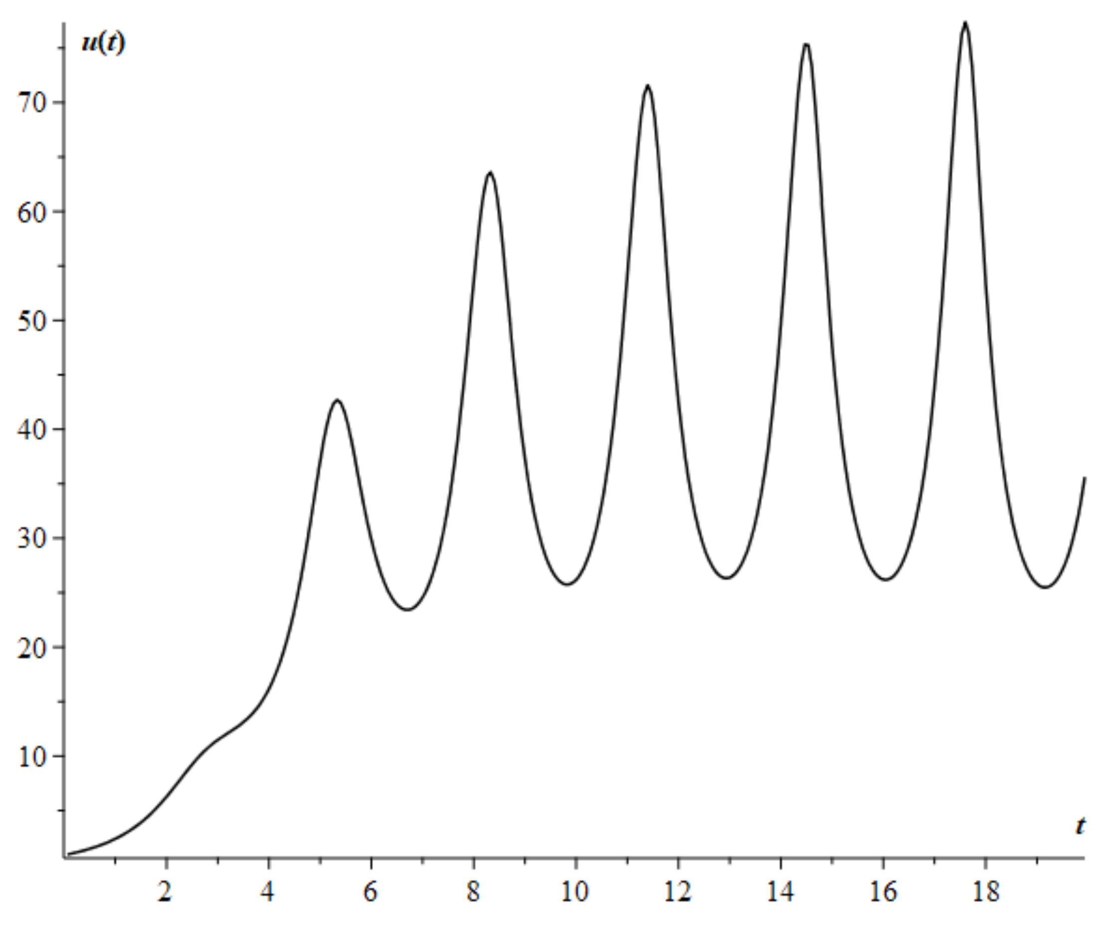
It should be noted that for this example, condition (10) is satisfied. The simulation results using Formula (17) give the calculated curve in Figure 3.
Figure 3 shows that the shape of the calculated curve has become noticeably more complicated in comparison with the calculated curve in Figure 1. This is primarily due to changes in the parameters of the model Equation (16) with time t.
However, despite the more complex form of the calculated curve, we can use it to describe cyclical dynamics, for example, in economics, to describe cycles and crises.
An estimate of the computational accuracy is given in Table 2.
From Table 2, we see that with an increase in the nodes of the computational grid, the error decreases, and the computational accuracy tends to unity, which corresponds to the results of Lemma 3.

5. Discussion

In the case of the stiff Cauchy problem (4), the method may not work correctly. For example, this can be seen in Figure 2, the case when the b parameter has a sufficiently large value ( b = 18 ). Here, the stability condition (10) is violated. Therefore, the question of the condition for the appearance of the stiff Cauchy problem (4) deserves a separate study.
Another very interesting question also deserves attention: how does the variable order of the fractional derivative affect the stability of the explicit finite-difference scheme (6)? It should be noted that the variable order α ( t ) is included in estimate (10) for the stability of the method. Here, it is worthwhile to study the stability of the proposed scheme (6) depending on the behavior of the function α ( t ) , for example, monotonicity or its periodicity, etc. Additionally, the function α ( t ) can have a singularity at zero.

6. Conclusions

An explicit finite-difference scheme for a fractional equation with a derivative of the variable fractional order of the Gerasimov–Caputo type was investigated. The questions of convergence and stability were investigated. It was shown that the scheme is conditionally stable and converges to the first order. The results were confirmed by examples and estimates of computational accuracy.
It can be concluded that an explicit finite-difference scheme can be used to calculate dynamic processes in environments with saturation. Further continuation of the work lies is the practical application of an explicit finite-difference scheme for calculating the curves of the volumetric activity of radon in a storage chamber by analogy with work [36].

Author Contributions

Conceptualization, R.P.; methodology, R.P.; software, D.T.; validation, D.T. and R.P.; investigation, D.T.; resources, D.T.; writing—original draft preparation, D.T.; writing—review and editing, R.P.; visualization, D.T.; supervision, R.P. All authors have read and agreed to the published version of the manuscript.

Funding

The work was carried out within the framework of the research project of the Vitus Bering Kamchatka State University Natural disasters of Kamchatka—earthquakes and volcanic eruptions (monitoring forecast, study, psychological support of the population) No. AAAA-A19-119072290002-9 and subject research IKIR FEB RAS “Physical processes in the system of near space and geospheres under solar and lithospheric influences” No. AAAA-A21-121011290003-0.

Conflicts of Interest

The authors declare no conflict of interest. The funders had no role in the design of the study; in the collection, analyses, or interpretation of data; in the writing of the manuscript, or in the decision to publish the results.

Abbreviations

The following abbreviations are used in this manuscript:
FO-VOFractional operator of variable order
IKIR FE RASInstitute of Cosmophysical Research and Radio Wave Propagation,
Far Eastern Branch of the Russian Academy of Sciences

References

  1. Oldham, K.; Spanier, J. The Fractional Calculus. Theory and Applications of Differentiation and Integration to Arbitrary Order; Academic Press: London, UK, 1974; p. 240. [Google Scholar]
  2. Miller, K.; Ross, B. An Introduction to the Fractional Calculus and Fractional Differntial Equations; A Wiley-Interscience Publication: New York, NY, USA, 1993; p. 384. [Google Scholar]
  3. Podlubny, I. Fractional Differential Equations: An Introduction to Fractional Derivatives, Fractional Differential Equations to Methods of Their Solution and Some of Their Applications; Academic Press: London, UK, 1998; p. 340. [Google Scholar]
  4. Kilbas, A.A.; Srivastava, H.M.; Trujillo, J.J. Theory and Applications of Fractional Differential Equations; Elsevier Science: New York, NY, USA, 2006; Volume 204, p. 540. [Google Scholar]
  5. Petras, I. Fractional-Order Nonlinear Systems. Modeling, Analysis and Simulation; Springer: Berlin/Heidelberg, Germany, 2011; p. 218. [Google Scholar]
  6. Machado, J.T.; Kiryakova, V.; Mainardi, F. Recent history of fractional calculus. Commun. Nonlinear Sci. Numer. Simul. 2011, 16, 1140–1153. [Google Scholar] [CrossRef] [Green Version]
  7. Uchaikin, V. Fractional Derivatives for Physicists and Engineers. Volume I Background and Theory; Springer: Berlin/Heidelberg, Germany, 2013; p. 373. [Google Scholar]
  8. Tarasov, V.E. Review of some promising fractional physical models. Int. J. Mod. Phys. B 2011, 27, 1330005. [Google Scholar] [CrossRef] [Green Version]
  9. Coimbra, C.F. Mechanics with variable-order differential operators. Annalen der Physik 2003, 12, 692–703. [Google Scholar] [CrossRef]
  10. Rossikhin, Y.A.; Shitikova, M.V. Application of fractional calculus for dynamic problems of solid mechanics: Novel trends and recent results. Appl. Mech. Rev. 2010, 63, 010801. [Google Scholar] [CrossRef]
  11. Parovik, R.I. Mathematical models of oscillators with memory. In Oscillators-Recent Developments; Salzenstein, P., Ed.; IntechOpen: London, UK, 2019; pp. 3–21. [Google Scholar]
  12. Glöckle, W.G.; Nonnenmacher, T.F. A fractional calculus approach to self-similar protein dynamics. Biophys. J. 1995, 68, 46–53. [Google Scholar] [CrossRef] [Green Version]
  13. Magin, R.L. Fractional calculus in bioengineering, Part 1–3. Crit. Rev. Biomed. Eng. 2004, 32, 1–377. [Google Scholar] [CrossRef] [Green Version]
  14. Makarov, D.V.; Parovik, R.I. Modeling of economic cycles using the theory of fractional calculus. J. Internet Bank. Commer. 2016, 21, S6. [Google Scholar]
  15. Tarasov, V.E. Mathematical Economics: Application of Fractional Calculus. Mathematics 2020, 8, 660. [Google Scholar] [CrossRef]
  16. Ortigueira, M.D.; Machado, J.T. What is a fractional derivative? J. Comput. Phys. 2015, 293, 4–13. [Google Scholar] [CrossRef]
  17. Samko, S.G.; Ross, B. Integration and differentiation of a variable fractional order. Integral Transforms Spec. Funct. 1993, 1, 277–300. [Google Scholar] [CrossRef]
  18. Patnaik, S.; Hollkamp, J.P.; Semperlotti, F. Applications of variable-order fractional operators: A review. Proc. R. Soc. A 2020, 476, 20190498. [Google Scholar] [CrossRef] [PubMed] [Green Version]
  19. Garrappa, R. Numerical Solution of Fractional Differential Equations: A Survey and a Software Tutorial. Mathematics 2018, 6, 16. [Google Scholar] [CrossRef] [Green Version]
  20. Cai, M.; Li, C. Numerical approaches to fractional integrals and derivatives: A review. Mathematics 2020, 8, 43. [Google Scholar] [CrossRef] [Green Version]
  21. Sun, H.; Chang, A.; Zhang, Y.; Chen, W. A review on variable-order fractional differential equations: Mathematical foundations, physical models, numerical methods and applications. Fract. Calc. Appl. Anal. 2019, 22, 27–59. [Google Scholar] [CrossRef] [Green Version]
  22. Valério, D.; Da Costa, J.S. Variable-order fractional derivatives and their numerical approximations. Signal Process. 2011, 91, 470–483. [Google Scholar] [CrossRef]
  23. Sun, H.; Chen, W.; Chen, Y. Variable-order fractional differential operators in anomalous diffusion modeling. Phys. A Stat. Mech. Appl. 2009, 388, 4586–4592. [Google Scholar] [CrossRef]
  24. Li, X.; Li, H.; Wu, B. A new numerical method for variable order fractional functional differential equations. Appl. Math. Lett. 2017, 68, 80–86. [Google Scholar] [CrossRef]
  25. Cao, J.; Qiu, Y. A high order numerical scheme for variable order fractional ordinary differential equation. Appl. Math. Lett. 2016, 61, 88–94. [Google Scholar] [CrossRef]
  26. Zhou, Y.; Suzuki, J.L.; Zhang, C.; Zayernouri, M. Implicit-explicit time integration of nonlinear fractional differential equations. Appl. Numer. Math. 2020, 156, 555–583. [Google Scholar] [CrossRef]
  27. Zhao, X.; Sun, Z.Z.; Karniadakis, G.E. Second-order approximations for variable order fractional derivatives: Algorithms and applications. J. Comput. Phys. 2015, 293, 184–200. [Google Scholar] [CrossRef]
  28. Samko, S.G. Fractional integration and differentiation of variable order. Anal. Math. 1995, 21, 213–236. [Google Scholar] [CrossRef]
  29. Gerasimov, A. Generalization of linear deformation laws and their application to internal friction problems. AS USSR Appl. Math. Mech. 1948, 12, 529–539. [Google Scholar]
  30. Caputo, M. Linear Models of Dissipation whose Q is almost Frequency Independent—II. Geophys. J. Int. 1967, 13, 529–539. [Google Scholar] [CrossRef]
  31. Parovik, R.I. On a finite-difference scheme for an hereditary oscillatory equation. J. Math. Sci. 2021, 253, 547–557. [Google Scholar] [CrossRef]
  32. Parovik, R.I. Explicit finite-difference scheme for the numerical solution of the model equation of nonlinear hereditary oscillator with variable-order fractional derivatives. Arch. Control Sci. 2016, 26, 429–435. [Google Scholar] [CrossRef] [Green Version]
  33. Parovik, R. Mathematical modeling of linear fractional oscillators. Mathematics 2020, 8, 1879. [Google Scholar] [CrossRef]
  34. Lin, Y.; Xu, C. Finite difference/spectral approximations for the time-fractional diffusion equation. J. Comput. Phys. 2007, 225, 1533–1552. [Google Scholar] [CrossRef]
  35. Tvyordyj, D.A. Hereditary Riccati equation with fractional derivative of variable order. J. Math. Sci. 2021, 253, 564–572. [Google Scholar] [CrossRef]
  36. Tverdyi, D.; Parovik, R.; Makarov, E.; Firstov, P. Research of the process of radon accumulation in the accumulating chamber taking into account the nonlinearity of its entrance. E3S Web Conf. 2020, 196, 02027. [Google Scholar] [CrossRef]
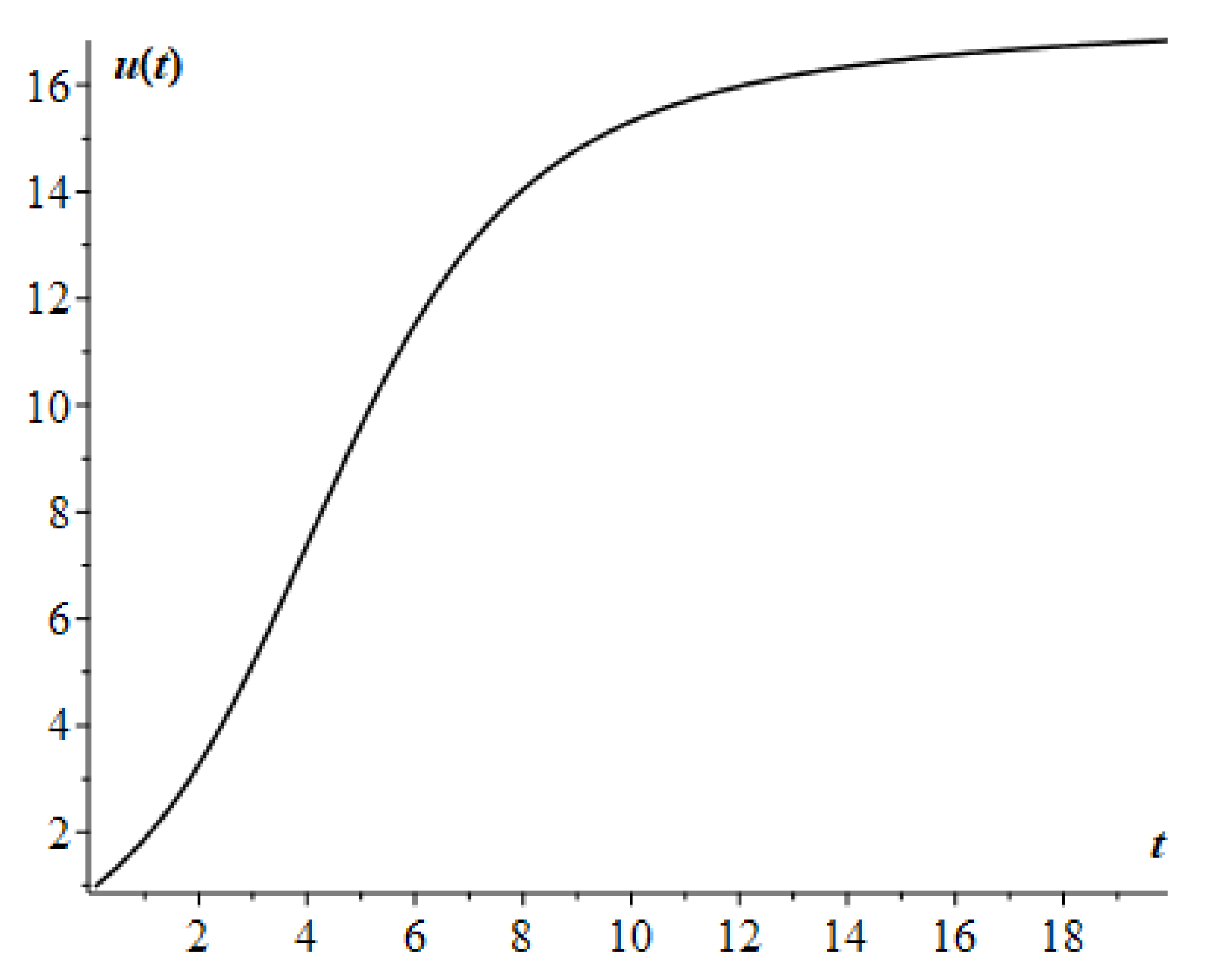
Figure 1. Fractional Riccati equation with constant coefficients and α = 0.8 , taking into account the fulfillment of condition (10).
Mca 26 00055 g001
Figure 2. Fractional Riccati equation with constant coefficients and α = 0.8 , taking into account the failure of condition (10).
Mca 26 00055 g002
Figure 3. Fractional Riccati equation with variable coefficients and α t = 0.9 0.5 t / T , taking into account the fulfillment of condition (10).
Mca 26 00055 g003
Table 1. Computational accuracy assessment p = ln ξ i ln ξ i ln ξ i + 1 ln ξ i + 1 .
iN τ ξ p
1101/100.039621-
2201/200.0239380.864994
3401/400.0134830.866691
4801/800.0073020.875344
51601/1600.0038650.885493
63201/3200.0020170.895208
76401/6400.0010430.903937
Table 2. Computational accuracy assessment p.
iN τ ξ p
1101/100.061331-
2201/200.0402040.868595
3401/400.0234170.856024
4801/800.0127510.860662
51601/1600.0066870.87111
63201/3200.0034350.882597
76401/6400.0017450.893334
Publisher’s Note: MDPI stays neutral with regard to jurisdictional claims in published maps and institutional affiliations.