Variational Bayesian Learning of SMoGs: Modelling and Their Application to Synthetic Aperture Radar

Abstract

We show how modern Bayesian Machine Learning tools can be effectively used in order to develop efficient methods for filtering Earth Observation signals. Bayesian statistical methods can be thought of as a generalization of the classical least-squares adjustment methods where both the unknown signals and the parameters are endowed with probability distributions, the priors. Statistical inference under this scheme is the derivation of posterior distributions, that is, distributions of the unknowns after the model has seen the data. Least squares can then be thought of as a special case that uses Gaussian likelihoods, or error statistics. In principle, for most non-trivial models, this framework requires performing integration in high-dimensional spaces. Variational methods are effective tools for approximate inference in Statistical Machine Learning and Computational Statistics. In this paper, after introducing the general variational Bayesian learning method, we apply it to the modelling and implementation of sparse mixtures of Gaussians (SMoG) models, intended to be used as adaptive priors for the efficient representation of sparse signals in applications such as wavelet-type analysis. Wavelet decomposition methods have been very successful in denoising real-world, non-stationary signals that may also contain discontinuities. For this purpose we construct a constrained hierarchical Bayesian model capturing the salient characteristics of such sets of decomposition coefficients. We express our model as a Dirichlet mixture model. We then show how variational ideas can be used to derive efficient methods for bypassing the need for integration: the task of integration becomes one of optimization. We apply our SMoG implementation to the problem of denoising of Synthetic Aperture Radar images, inherently affected by speckle noise, and show that it achieves improved performance compared to established methods, both in terms of speckle reduction and image feature preservation.

1. Introduction

Sparse decompositions of signals, images, and data have found widespread use across a wide array of scientific disciplines and practical applications. The key insight is that while modern sensors generate signals containing an often overwhelming amount of data, the useful information in them can often be described by a much smaller number of ‘primitives’. Early work in the compression, representation, and cleaning of seismic and other nature-generated signals, for example, has lead to the discovery of wavelets, bases that span signal spaces in a very efficient manner. A central modern motivation for sparsity comes from applications such as compressed sensing and computation (sparse recovery). The idea in sparse representation is to describe the original signals using such ‘atomic decompositions’, with the coefficients of the decomposition serving as the resultant ‘code’. This code is almost always sparse for a wide variety of signals, meaning that most coefficients will be almost zero with only a small percentage of them being significantly larger than zero. Statistically, the empirical histograms of those sets of coefficients are highly peaked at zero. Our aim in this paper is to use appropriate probability density functions to describe such distributions. We would also like to incorporate notions of uncertainty in the model parameters. For that purpose we propose to use the sparse mixture of Gaussians (SMoG) model as a flexible prior on the decomposition coefficients, learnt under the Bayesian framework. Olshausen and Millman [1] have used this prior for learning sparse codes of natural images under a combined Maximum Likelihood/Markov Chain Monte Carlo (MCMC) framework. Roussos, Roberts and Daubechies [2] have used a similar model for functional MRI data, employing wavelet decompositions in an independent component analysis setting, but learned under a Variational Bayes framework. A wide range of other applications have used similar models from a maximum likelihood, maximum a-posteriori, and expectation-maximization perspective. In this paper we give a detailed description of the SMoG method and its implementation and place it in the wider context of computational statistical inference.

Bayesian inference is mainly concerned with posterior inference, using Bayes’ theorem as our vehicle [3]. This formally encodes the update of our prior knowledge in light of new data. We express our prior beliefs regarding the various uncertain quantities of our models in the form of Bayesian priors. The data, on the other hand, are probabilistically linked with the parameters of our models using the likelihood. A defining characteristic of the Bayesian approach is, therefore, that model parameters are regarded as random quantities, described by distributions. This distinguishes Bayesian learning from standard frequentist approaches. In the Bayesian approach learning and inference are treated exactly the same.

Posterior elicitation, however, puts on us the burden of computing often intractable, high-dimensional integrals, as we need to integrate out certain model parameters and hidden variables, often regarded as ‘nuisance variables’. A number of methods have been developed from the Bayesian community to tackle this problem, ranging from deterministic ones, such as the Laplace approximation, to stochastic, the main representative of which are the various MCMC approaches. While extremely powerful, MCMC methods are also computationally demanding. Another deterministic approach, based on principles of Statistical Physics, which is more flexible than the Laplace approximation while being much more computationally efficient than MCMC, is offered by variational methods [4,5]. These make mean-field approximations to the Bayesian evidence and joint posteriors to derive a rigorous lower-bound to the evidence and a set of ‘self-consistent’ update equations for the unknowns of the problem. It should be noted here that the term ‘approximate’ does not refer to the accuracy of the results, which is generally better than the classical ones, due to the integration of knowledge and uncertainty, but only to the way in which the integrals are calculated.

The rest of the paper derives the general variational Bayesian (VB) framework and then applies it to the particular problem of learning the sparse mixture of Gaussians model, with a special emphasis to encoding sets of coefficients from sparse signal representations of Earth observation signals. Earth observation data, such as those from SAR, LiDAR, GNSS time series, etc, are inherently noisy. In this paper, we focus on the problem of speckle reduction in Synthetic Aperture Radar imagery, an increasingly important, high-resolution Earth sensing modality for mapping and monitoring. The extremely complex nature of terrestrial mechanisms and phenomena, such as tectonic shifts and deformations and their corresponding magmatic masses, for example, make the use of sophisticated denoising methods necessary for the extraction of the underlying signals.

2. Variational Bayesian Learning of SMoGs

In this section we present a hierarchical Bayesian model for modelling sparse sets of decomposition coefficients in a basis, e.g., wavelet coefficients. The general problem we want to solve is the following: given a noisy signal, $\mathbf{y}\in {\mathbb{R}}^N$, and a basis, $\mathbf{\Phi }=\left\{{\mathbf{\phi }}_{\lambda }\right\}$, our goal is to infer the posterior distribution of the wavelet decomposition coefficients, $\left\{c_{\lambda }\right\}$, such that the unknown clean signal, $\mathbf{x}$, is recovered, under the modelling constraint that it is efficiently, i.e., sparsely, described in the given basis.

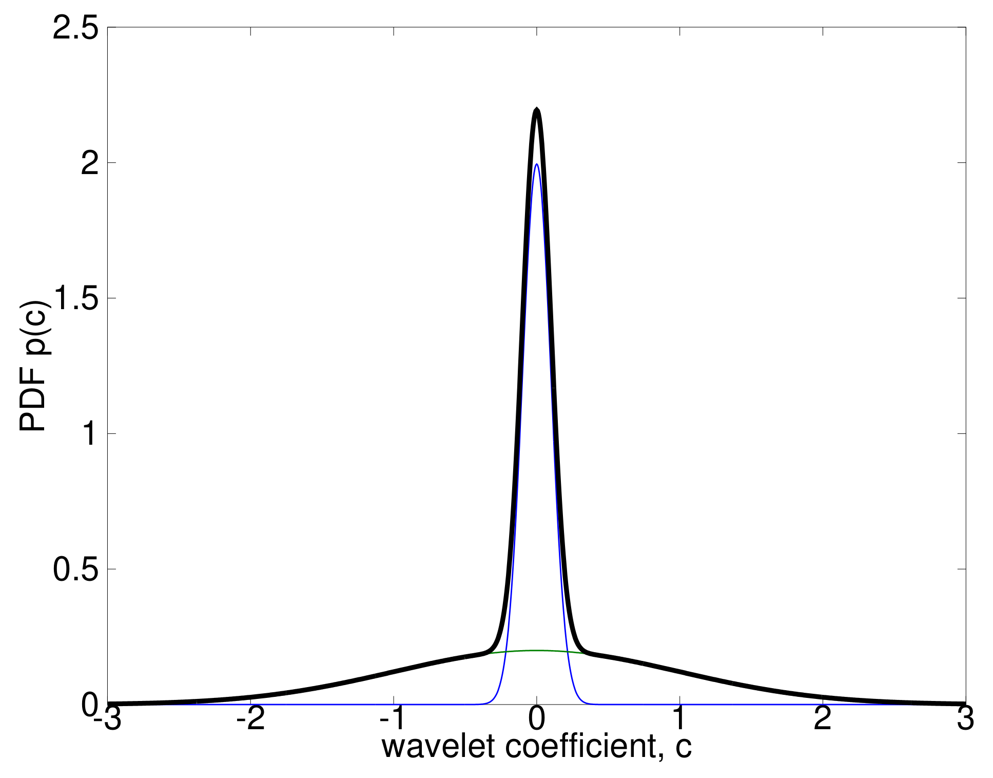
2.1. Bayesian Modelling of Sparse Wavelet Coefficients

2.1.1. The Bayesian SMoG Model

The model should capture the desired or expected properties of those sets of expansion coefficients in the prior, informed by the observed behaviour of those decompositions in practice. It should also be constrained enough to enforce sparsity while at the same time being flexible enough to capture a wide range of decompositions of a variety of signals.

A flexible prior that is at the same time mathematically tractable is a mixture distribution. For an M–component model, a mixture-of-Gaussians (MoG) can be expressed mathematically as a linear combination of component densities,

$$p\left(y_n\right|{\mathbf{\theta }}_{\mathrm{SMoG}})=\sum _{m=1}^M{\pi }_m \mathcal{N}\left(y_n;{\mu }_m,\frac{1}{{\beta }_m}\right),$$

(1)

where $({\mu }_m,{\beta }_m)$ are the mean and precision (inverse variance) parameters of the m–th Gaussian component over $y_n$ and ${\left\{{\pi }_m\right\}}_{m=1}^M$ are mixing proportions. Since the ${\pi }_m$s are non-negative the MoG is also a convex combination of Gaussians. We collect the learnable parameters in a vector ${\mathbf{\theta }}_{\mathrm{SMoG}}=\{\mathbf{\pi },\mathbf{\mu },\mathbf{\beta }\}$. Each component in the mixture may be interpreted as a ‘state’. In our implementation we enforce sparsity by restricting the general mixture of Gaussians model to be a two-component, zero co-mean mixture: one component, with small variance, captures non-active coefficients while the other, with large-variance, capture active ones. Olshausen and Millman also propose a ternary version of the MoG model for sparse coding in [1], in which the data can assume three states: non-active, active negative and active positive; see Figure 1b. That is, while the ‘off’ mode is the same as before, the ‘on’ mode has two sub-modes. The hope here is that this PDF will better describe the behaviour of coding coefficients, focusing on the meso-scale coefficients. However, Olshausen and Millman reported minimal benefits from this added complexity. Therefore, we will use a two-state model in this paper. In [1] the state variables of the ternary model are inferred using Gibbs sampling while the model parameters are learnt by a gradient, maximum likelihood algorithm. In this paper, we instead employ a fully Bayesian model and learning algorithm to the problem.

In multiscale, wavelet-type analysis, a separate SMoG is placed on each dyadic scale, resulting in a collection of parameters, ${\theta }_{\mathrm{SMoG}}={\bigcup }_j{\theta }_{{\mathrm{SMoG}}_j}$, and adapted to the characteristics of the particular signal. We name our model a sparse MoG (SMoG). The Bayesian SMoG model probability density is shown in Figure 1.

Introducing Hidden Variables

In order to derive a computationally efficient learning algorithm, we first start by performing the following ‘thought experiment’: if we had access to the state of each data point, as being active or non-active, the task of learning the parameters of the two components would be much easier, as the two components would then be decoupled and we would only need to learn the parameters of the individual component that the data points would be assumed to have been generated from. We will regard those unknown states as ‘missing’ data and introduce a set of latent indicator variables, ${\xi }_n$, such that when “filled in” by our algorithm, we will achieve our goal. The component indicators therefore play a very important role in this model. They essentially signify the component, m, at which the data point n becomes (probabilistically) assigned to; that is, in the case of SMoGs for wavelet analysis, whether a particular wavelet basis ${\mathbf{\phi }}_{\lambda }$ is significant or not for a specific dataset. This decision happens at the ‘inference’ stage of the Bayesian algorithm, via the corresponding posterior distribution, i.e., after the model has seen the data. The latent variables ${\xi }_n$ effectively work as ‘switches’, turning wavelet bases ‘on’ or ‘off’ for a particular signal. The likelihood for the SMoG model after the introduction of the latent variables becomes:

$$p\left(y_n\right|{\theta }_{\mathrm{SMoG}})=\sum _{m=1}^{M}p({\xi }_n=m|\mathbf{\pi }) p\left(y_n|{\xi }_n,\mathbf{\mu },\mathbf{\beta }\right).$$

(2)

Each component indicator, ${\xi }_n$, “picks” one of M components for its corresponding data point $y_n$ with a-priori probability $p({\xi }_n=m|\mathbf{\pi })$, for all n.

Probability Assignments

We will formulate our SMoG model as a Dirichlet mixture model. In Bayesian modelling, the assumed distribution of the latent variables as well as the priors over the parameters of the model must be stated, as they are an integral part of the model itself. The indicator variables of the SMoG components, $\mathbf{\xi }=\left({\xi }_n\right)$, are assigned a categorical (or, generalized Bernoulli) distribution, such that $p({\xi }_n=m|\mathbf{\pi })={\pi }_m$, $\forall n$. The above can be thought of as the soft assignment $n\mapsto m$, of the nth data point to the mth component, with probability $p({\xi }_n=m|\mathbf{\pi })$. This prior can be more conveniently written as

$$p\left(\mathbf{\xi }\right|\mathbf{\pi })\doteq \mathrm{Cat}\left(\mathbf{\pi }\right)=\prod _{n=1}^N{{\pi }_m}^{[{\xi }_n=m]},$$

(3)

where the symbol $[·]$ is the Iverson bracket, which is equal to 1 if its argument is true and 0 otherwise. This form offers some conceptual advantages with respect to expressing conjugacies in the model and facilitates further mathematical manipulations.

The prior over the model parameters, ${\theta }_{\mathrm{SMoG}}$, as directly read from the SMoG DAG, is

$$p(\mathbf{\pi },\mathbf{\mu },\mathbf{\beta })=p\left(\mathbf{\pi }\right)\left(p\left(\mathbf{\mu }\right)p\left(\mathbf{\beta }\right)\right)=p\left(\mathbf{\pi }\right)\left(\prod _{m=1}^{M}p\left({\mu }_m\right)\prod _{m=1}^{M}p\left({\beta }_m\right)\right),$$

(4)

with the following assignments:

• The prior over the mixing proportions vector, $\mathbf{\pi }$, is a Dirichlet distribution with concentration hyperparameters $\mathbf{\alpha }=({\alpha }_1,\dots ,{\alpha }_M)$, with ${\alpha }_m\ge 0$:

  $$p\left(\mathbf{\pi }\right|\mathbf{\alpha })\doteq \mathrm{Dir}(\mathbf{\pi };\mathbf{\alpha })=\frac{1}{\mathrm{B}\left(\mathbf{\alpha }\right)}\prod _{m=1}^M{{\pi }_m}^{{\alpha }_m-1},\mathrm{B}\left(\mathbf{\alpha }\right)=\frac{{\prod }_{m=1}^M⯀\left({\alpha }_m\right)}{⯀\left({\sum }_{m=1}^M{\alpha }_m\right)},$$

  (5)

  where $⯀(·)$ and $\mathrm{B}(·)$ are the Gamma and multivariate Beta functions, respectively. The Dirichlet is sometimes called a ‘distribution over distributions’, since it is a probability distribution on the simplex of sets of non-negative numbers that sum to one [6]. In other words, each draw from a Dirichlet is itself a distribution. It is the conjugate prior of the Categorical distribution [3]. Note that in the SMoG model, in contrast to the general MoG, it is more logical to assign different hyperparameters ${\alpha }_m$ for the different components, $m=1$ and $m=2$, in the binary case, i.e., have an asymmetric prior because, for sparse data, we expect that most of the bases should be inactive (‘off’). Therefore, we assign a much larger a-priori concentration parameter, ${\alpha }_1$, corresponding to the peak of the distribution at zero, than ${\alpha }_2$. This means that the a-priori probability of drawing an inactive coefficient $c_{\lambda }$ from the model is significantly higher than drawing an active one.
• The prior over each component mean, ${\mu }_m$, is a Gaussian, with hyperparameters $(m_0,{\tau }_0)$ such that the hyperparameter $m_0$ of the prior is $m_0\doteq 0$, implying ${\mathbb{E}}_p\left[\mu \right]=0$, while we let the algorithm learn the posterior hyperparameters of $q\left(\mu \right)$. That is, we do not fix the means themselves to 0 but only the prior hyperparameters and let the algorithm learn the actual value of the corresponding posterior hyperparameters itself using an empirical Bayes approach. The above expresses our prior belief that the centres of the distribution of the $c_{\lambda }$ are drawn from a hyperprior with mean zero and a small width, ${\tau }_0$. This reflects the empirical observation that, for sparse signals, it is highly probable that most wavelet coefficients will be zero:

  $$p\left({\mu }_m\right)\doteq \mathcal{N}({\mu }_m;m_0,{\tau }_0)=\frac{1}{\sqrt{2\pi /{\tau }_0}}{\mathrm{e}}^{-\frac{1}{2}{\tau }_0{({\mu }_m-m_0)}^2}.$$

  (6)
• The prior over each component precision, ${\beta }_{jm}$, of the jth dyadic scale is a Gamma distribution with hyperparameters $(b_0,c_0)$. While in general we would often express our lack of prior information in the scales of the $\beta$ parameters by selecting a vague (‘uninformative’) prior [7], in this case we want to express our expectation that, for sparse signals, again, only a few wavelet coefficients will be significantly different from zero. Therefore, we will select the prior hyperparameters $(b_0,c_0)$ such that the non-active coefficients $c_{\lambda }$, which will form the majority of the representation, will be neatly concentrated around 0, i.e., assign a high precision to that state, while the few ‘large’ ones will be drawn from a component with a small precision (high variance), to allow “wiggle space”:

  $$p\left({\beta }_m\right)\doteq \mathrm{Ga}({\beta }_m;b_0,c_0)=\frac{1}{⯀\left(b\right)b_0^{c_0}}{\beta }_m^{c_0-1}{\mathrm{e}}^{-\frac{1}{b_0}{\beta }_m},$$

  (7)

  where we have used the scale-shape parameterization of the Gamma distribution.

2.1.2. SMoG Bayesian Network

We will express our hierarchical Bayesian model as a directed acyclic graph that is a particular type of a probabilistic graphical model (PGM) called a Bayesian network, capturing the probabilistic dependence relations among the random variables in our model. In PGMs a node represents a random variable and an edge a statistical dependence. In a Bayesian network, each node has a set of ‘parent’ and a set of ‘children’ nodes. The conditional probability of a variable, v, in the model given other variables is represented by that node given its parents, $\mathrm{pa}\left(v\right)$. We next introduce the important concept of a Markov blanket: the Markov blanket of a node is the set of its parents, children, and co-parents (i.e., the other parents of its children). A Markov blanket defines a notion of ‘neighborhood’ in Bayesian networks: the probability of a random variable is independent of all other variables outside of its Markov blanket. These concepts will prove to be essential during learning and inference because they localize computations. The Bayesian network for the model in Figure 2.

2.2. Variational Bayesian Inference

We now show how variational ideas can be used in order to construct methods for approximating the integrals necessary for Bayesian learning [4,5]. In variational Bayesian (VB) learning, the objective function to be optimized is the negative free energy (NFE) of the system, $\mathcal{F}$. The NFE forms a lower bound to the log-evidence of the model, $logp\left(\mathcal{Y}\right)$, and is therefore the Bayesian quantity that we seek to maximize: see Figure 3.

We will now show how the NFE is derived. Starting from the marginal likelihood, $\mathcal{L}=p\left(\mathcal{Y}\right)$ and expanding it in terms of the joint distribution over the the full generative probabilistic model, represented in the directed graphical model $\mathcal{G}$, including the unknowns, $\mathcal{U}=\mathcal{X}\cup \Theta$ (comprising the latent variables and the model parameters), and the data, $\mathcal{Y}$, we find the important relation

$$\underset{log-\mathrm{evidence}}{\underbrace{logp\left(\mathcal{Y}\right)}}=\underset{\mathrm{Negative}\mathrm{free}\mathrm{energy}}{\underbrace{\mathcal{F}\left[q\left(\mathcal{U}\right)\right]}}+\underset{\mathrm{Kullback}--\mathrm{Leibler}\mathrm{divergence}\ge 0}{\underbrace{\mathrm{KL}\left[q\left(\mathcal{U}\right)\parallel p\left(\mathcal{U}\right|\mathcal{Y})\right]}}.$$

(8)

The second term in the equation above expresses the “distance” between the variational posterior, $q\left(\mathcal{U}\right)$, and the true posterior, $p\left(\mathcal{U}\right|\mathcal{Y})$, quantified by the Kullback–Leibler divergence, or relative entropy, $\mathrm{KL}\left[q\parallel p\right]$. (Note that the $\mathrm{KL}$ divergence is not symmetric with respect to commuting its arguments: $\mathrm{KL}(p\parallel q)\ne \mathrm{KL}(q\parallel p)$. The particular form used in the VB method is the one that forces the variational posterior to cover the majority of the probability mass under the true posterior and also allows for easier mathematical derivations.) This is a non-negative quantity; therefore the NFE is a rigorous lower bound to the log-evidence. If the variational posterior equals the true posterior, the NFE is the log-evidence. Of course, for all but the simplest statistical models certain approximations have to be made in order for inference to be tractable. By choosing a set of approximate distributions that facilitates easier computations, usually by choosing convenient functional forms, such as PDFs in the exponential family, or/and breaking some dependencies in the joint model, the KL divergence becomes non-zero and the NFE lowers. Our goal in Bayesian modelling is first to judiciously choose the above aspects of our model and then maximize $\mathcal{F}\left[q\left(\mathcal{U}\right)\right]$, in order to obtain the tightest possible bound, within the chosen set of distributions. Focusing on the NFE, this can be expressed as

$$\mathcal{F}\left[q\left(\mathcal{U}\right)\right]=\underset{\mathrm{Variational}\mathrm{Energy},\mathcal{E}\left[\mathrm{p}\left(\mathcal{G}\right)\right]}{\underbrace{{〈logp\underset{\underset{\mathcal{G}}{︸}}{(\mathcal{U},\mathcal{Y})}〉}_q}}+\underset{\mathrm{Shannon}\mathrm{entropy},\mathcal{H}\left[\mathrm{q}\left(\mathcal{U}\right)\right]}{\underbrace{{〈-logq\left(\mathcal{U}\right)〉}_q}}.$$

(9)

The first term in the above equation, the expected log-probability of the model, i.e., the log-joint $logp\left(\mathcal{G}\right)$, with respect to the variational posterior, is called the variational energy and the second term is the Shannon entropy (information entropy) of the variational posterior over the unknowns. Since the nodes $\mathcal{Y}$ are instantiated to the data, and are therefore fixed quantities, the above integration gives us a functional that maps PDFs in the function space of candidate approximate joint distributions, $\mathcal{Q}=\left\{q\right(\mathcal{U}\left)\right\}$, to ${\mathbb{R}}_{+}$. This functional we be maximized using functional differentiation below. We will find it computationally convenient later to further decompose the NFE into the following formula:

$$\mathcal{F}\left[q\left(\mathcal{U}\right)\right]={\overline{\mathcal{L}}}_{\Theta }\left(\mathcal{X},\mathcal{Y}\right)+\mathcal{H}\left[q\left(\mathcal{X}\right)\right]-\mathrm{KL}\left[q(\Theta )\parallel p(\Theta )\right],$$

(10)

where ${\overline{\mathcal{L}}}_{\Theta }\left(\mathcal{X},\mathcal{Y}\right)\stackrel{\mathrm{def}}{=}{〈logp(\mathcal{X},\mathcal{Y}|\Theta )〉}_q$ is the posterior-averaged complete-data log-likelihood. This form will be useful for the evaluation of the NFE itself later.

Under the mean-field ansatz,

$$q\left(\mathcal{U}\right)\doteq \prod _{\alpha }{q}_{{}_{\alpha }}\left({\mathbf{u}}_{\alpha }\right),$$

(11)

where the posterior is factorized over subsets of the unknowns, $\mathcal{U}\doteq {\bigcup }_{\alpha }{\mathbf{u}}_{\alpha }$, it can be shown that our objective function, $\mathcal{F}$, can be further written as

$$\mathcal{F}\left[q\left(\mathcal{U}\right)\right]=\sum _{\alpha }\mathrm{KL}\left[exp\left({〈logp\left(\mathcal{U},\mathcal{Y}\right)〉}_{q(\mathcal{U}\setminus \left\{{\mathbf{u}}_{\mathbf{f}\mathbf{f}}\right\})}\right)\parallel q_{{}_{\alpha }}\left({\mathbf{u}}_{\alpha }\right)\right]+c;$$

(12)

in other words, the dependence of $\mathcal{F}$ on the individual $q_{{}_{\alpha }}$s is only via their corresponding $\mathrm{KL}$ divergencies. Taking the functional derivative and equating it to 0, under the constraint that each $q_{\alpha }$ integrates to one (for it to be a proper probability distribution),

$$\frac{\delta }{\delta q\left({\mathbf{u}}_{\mathbf{f}\mathbf{f}}\right)}\left\{\mathcal{F}\left[q\left({\mathbf{u}}_{\mathbf{f}\mathbf{f}}\right)\right]+{\lambda }_{\alpha }\left(\int q\left({\mathbf{u}}_{\mathbf{f}\mathbf{f}}\right)\mathrm{d}{\mathbf{u}}_{\mathbf{f}\mathbf{f}}-1\right)\right\}\doteq 0,$$

(13)

and by the fundamental lemma of calculus of variations [8], we obtain the corresponding Euler–Lagrange equation for the problem [9]. This in our case simplifies by the fact that the functional does not depend on the derivatives $q_{\alpha }^{\prime }$. Moreover, based on the observation above that the NFE is maximized when the KL divergence is zero, and plugging that into the above two equations, we obtain the final general expression for the optimal variational posteriors:

$$q_{\alpha }^{☆}\left({\mathbf{u}}_{\mathbf{f}\mathbf{f}}\right)=\frac{1}{{\mathcal{Z}}_{\alpha }}exp\left({〈logp\left(\mathcal{U},\mathcal{Y}\right)〉}_{q(\mathcal{U}\setminus \left\{{\mathbf{u}}_{\mathbf{f}\mathbf{f}}\right\})}\right);$$

(14)

that is, we integrate over all the other variables with respect to their variational posterior. We see that by following the VB approach we have transformed an inference problem into an optimization one, which is often easier to solve.

The above generic equations of VB learning are then specialized for the particular model at hand. That is, based on the Markov relations in the Bayesian network, $\mathcal{G}$, corresponding to our problem, we can immediately write down the terms arising from the logarithm inside the angle brackets of Equation (14) and the Markov factorizations in $\mathcal{G}$. Note that these Markovian relations refer to the prior, and not to the mean-field variational assumptions regarding the posterior, which enter the picture only via the mean-field averaging, ${\langle ·\rangle }_q$. In terms of implementation, Equation (14) basically means that in order to compute the update equation for some unknown $\mathbf{u}$, $q\left(\mathbf{u}\right)$, we just need to apply the following generic procedure:

• Take the log-joint probability, $logp(\mathcal{Y},\mathcal{U})$, expand it into the various terms that correspond to the unkowns ${\mathbf{u}}_{\alpha }\in \mathcal{U}$, $\alpha =1,\dots ,\left|\mathcal{U}\right|$, and, for each $\alpha$, keep only its ‘relevant’ terms, i.e., the terms that contain expressions containing the variable ${\mathbf{u}}_{\alpha }$. These are none other than the nodes in the Markov blanket of the node ${\mathbf{u}}_{\alpha }$.
• Take the posterior averages, ${\langle ·\rangle }_q$, of the various terms. If the model is constructed such that the node conditional PDFs (i.e., given their parents) are in the conjugate-exponential family of distributions, these averages will be analytically computable.
• Rearrange and combine the various sub-terms so that we end up with expression patterns that correspond to known distributions, such as those in the exponential family, to finally find the expression of the update equation for each $q_{\alpha }\left({\mathbf{u}}_{\alpha }\right)$.

Note that if the model is constructed such that it belongs to the conjugate-exponential family of distributions, then the functional forms of the variational posteriors will be of the same form as their corresponding priors. Essentially, computing the posteriors is equivalent to shifting the priors to a position that balances both the requirement of fidelity with respect to reconstructing the data and the constraints imposed by the prior. This will be directly reflected in the form of the update equations. This means that the variational posterior hyperparameters, ${\widehat{\mathbf{\psi }}}_{\alpha }$, will be ‘moves’ in hyperparameter space, during learning, i.e., shifted versions of the corresponding prior hyperparameters, ${\mathbf{\psi }}_{\alpha ,0}$, updated according to the observed data:

$${\widehat{\mathbf{\psi }}}_{\alpha }={\mathbf{\psi }}_{\alpha ,0}\oplus g\left(\mathbf{y}\right),$$

(15)

where ‘⊕’ is a generalized addition operator, denoting the fusion of information from the prior and likelihood of node $\alpha$, and $g\left(\mathbf{y}\right)$ denotes a generic function of the data—these are specialized for each particular model.

2.3. Applying VB Learning to the SMoG Model

Applying the above general methodology and equations to the particular case of Bayesian SMoGs (where the graphical model is shown in Figure 2), we obtain the concrete expressions for the NFE and the update equations for the nodes of ${\mathcal{G}}_{\mathrm{SMoG}}$ for this model.

In particular, the ensemble of latent variables and parameters of the model is $\mathcal{U}=\{\mathbf{\xi },\mathbf{\theta }\}$. Under the mean-field assumption (Beal, [5]), the variational posterior, $q\left(\mathcal{U}\right)$, factorizes over the elements of $\mathcal{U}$ and, therefore, factors in each unknown can be maximized individually:

$$q\left(\mathcal{U}\right)=q\left(\mathbf{\xi }\right)q(\mathbf{\pi },\mathbf{\mu },\mathbf{\beta }),$$

(16)

Note that, contrary to popular belief, we do not need to make a factorization assumption over $\mathbf{\theta }=\{\mathbf{\pi },\mathbf{\mu },\mathbf{\beta }\}$, but only over $\{\mathbf{x},\mathbf{\theta }\}$; the factorization amongst the parameters “falls out” of the Markovian structure of the DAG [5].

Now, the joint probability of ${\mathcal{G}}_{\mathrm{SMoG}}$, by inspecting the dependencies of the graphical model, is:

$$p\left({\mathcal{G}}_{\mathrm{SMoG}}\right)=p({\mathcal{U}}_{\mathrm{SMoG}},{\mathcal{Y}}_{\mathrm{SMoG}})=p\left(\mathbf{y}\right|\mathbf{\xi };\mathbf{\mu },\mathbf{\beta })p\left(\mathbf{\xi }\right|\mathbf{\pi })p\left(\mathbf{\pi }\right)p\left(\mathbf{\mu }\right)p\left(\mathbf{\beta }\right),$$

(17)

where the conditional likelihood (the data likelihood conditioned on the latent variables) is

$$p\left(\mathbf{y}\right|\mathbf{\xi };\mathbf{\mu },\mathbf{\beta })=\prod _{n=1}^{N}p\left(y_n\right|{\xi }_n;{\mu }_m,{\beta }_m).$$

(18)

This product is represented by the plate over $\left\{n\right\}$ in the graphical model of Figure 2.

The NFE for the SMoG model, given the above graph-structured set of RVs and their corresponding joint probability distribution, $p\left(\mathcal{G}\right)$, now becomes

$$\begin{array}{ccc}\hfill \mathcal{F}& =& \left({〈logp\left(\mathbf{y}|\mathbf{\xi };\mathbf{\mu },\mathbf{\beta }\right)〉}_{q\left(\mathbf{\xi }\right)q\left(\mathbf{\mu }\right)q\left(\mathbf{\beta }\right)}+{〈logp\left(\mathbf{\xi }|\mathbf{\pi }\right)〉}_{q\left(\mathbf{\xi }\right)q\left(\mathbf{\pi }\right)}\right)+\hfill \\ & & \mathcal{H}\left[q\left(\mathbf{\xi }\right)\right]-\hfill \\ & & \left(\mathrm{KL}\left[q\left(\mathbf{\pi }\right)\parallel p\left(\mathbf{\pi }\right)\right]+\mathrm{KL}\left[q\left(\mathbf{\mu }\right)\parallel p\left(\mathbf{\mu }\right)\right]+\mathrm{KL}\left[q\left(\mathbf{\beta }\right)\parallel p\left(\mathbf{\beta }\right)\right]\right).\hfill \end{array}$$

(19)

The first two terms are the average complete-data likelihood, ${\overline{\mathcal{L}}}_{\Theta }\left(\mathcal{X},\mathcal{Y}\right)$, defined above, each latent variable provides an entropy term, and each parameter provides a minus $\mathrm{KL}$ divergence. The above expression is equivalent to the (negative of) the Helmholtz free energy in Statistical Physics,

$$\mathcal{F}=- 〈logp\left({\mathcal{V}}_{\mathcal{G}}\right)〉+\mathcal{H}\left[q\left(\mathcal{U}\right)\right],$$

where the first term is minus the ‘variational energy’ and the second is the ‘variational entropy’. Note that the above Equation (19) is expressed in terms of the form $〈logp\left({\mathbf{v}}_{\beta }|\mathrm{pa}\left({\mathbf{v}}_{\beta }\right)\right)〉$ and $〈logq\left({\mathrm{v}}_{\alpha }\right)〉$, where $\beta \in \{1,\dots ,|\mathcal{U}\cup \mathcal{Y}\left|\right\}$ and $\alpha \in \{1,\dots ,|\mathcal{U}\left|\right\}$. That is, they correspond to internal and leaf nodes of the SMoG DAG, respectively. We will exploit this observation in our implementation later.

2.3.1. Update Equations for the Unknowns of the Model

We now use the generic update equation for the optimal variational posteriors, Equation (14), derived in the previous section, and specialize it for our model. As an example, the derivation of the update equations for the precisions, $\mathbf{\beta }$, will be shown here in detail; the remaining equations are derived similarly.

We first rewrite Equation (14), with $\mathbf{u}\leftarrow \mathbf{\beta }$, Ref. [10] as

$$q^{☆}\left(\mathbf{\beta }\right)\propto exp\left[{〈logp\left(\mathbf{\xi },\mathbf{y}|\mathbf{\beta }\right)〉}_{q\left(\mathbf{\xi }\right)}+logp\left(\mathbf{\beta }\right)\right],$$

(20)

where the first term is the expected ‘complete-data’ likelihood for $\mathbf{\beta }$, $\overline{\mathcal{L}}\left[\mathbf{\beta }\right]$. (Here we just break up the general expression for the variational posteriors,

$$q^{☆}\left(\mathbf{u}\right)\propto exp\left({〈logp\left(\mathcal{U},\mathcal{Y}\right)〉}_{q(\mathcal{U}\setminus \{\mathbf{u}\left\}\right)}\right),$$

into a prior factor for the particular unknown times a likelihood term, which is reminiscent of the Bayes’ rule.) This formulation is mainly used here for demonstrating a simple derivation of the formulæ. This is reminiscent of the so-called Q–function of the expectation-maximization (EM) algorithm, $Q\left({\mathbf{\theta }}^k\right)\stackrel{\mathrm{def}}{=}{\mathbb{E}}_{p\left(\mathcal{X}\right|\mathcal{Y})}\left[logp\left(\mathcal{X},\mathcal{Y}{\mathbf{\theta }}^{k-1}\right)\right]$, $k=1,\dots$, where the parameter $\mathbf{\theta }$ at the right-hand-side is instantiated in the value obtained in the previous iteration. In that method, one then takes the gradient with respect to the parameter ${\mathbf{\theta }}^k$ and equates it to zero, to obtain the current point estimate of $\mathbf{\theta }$ [11]. In the variational Bayesian approach, we instead use the full sufficient statistics to obtain posterior distributions. We will say more about the relation between the VB method and EM later.

Now, the complete-data log-likelihood for a single component ${\beta }_m$ is

$$logp\left(\mathbf{\xi },\mathbf{y}|{\beta }_m\right)=\frac{1}{2}\sum _{n=1}^{N}log{\beta }_m-\frac{1}{2}{\beta }_m\sum _{n=1}^N{\left(y_n-{\mu }_m\right)}^2,$$

due to the i.i.d. data. Therefore, averaging the above over the variational posterior, implies that $\overline{\mathcal{L}}\left[\mathbf{\beta }\right]$ can be written as

$$\overline{\mathcal{L}}\left[\mathbf{\beta }\right]=\sum _{m=1}^M\overline{\mathcal{L}}\left[{\beta }_m\right].$$

(21)

Responsibility-Weighted Statistics

In order to evaluate the $\overline{\mathcal{L}}\left[{\beta }_m\right]$’s, and equivalent quantities for the other variables in the model, we need the following intermediate quantities. We define the responsibility of component m with respect to data point n as the posterior probability value

$${\widehat{\gamma }}_{nm}=q({\xi }_n=m),\forall n,m,$$

(22)

seen as ‘soft’ assignments of data points to components. This will be implemented as conditional probability tables (CPTs). We now define the following responsibility-weighted statistics (resulting from integrating the data statistics over $\mathbf{\xi }$ wrt $q\left(\mathbf{\xi }\right)$ and over ${\mu }_m$ wrt $q\left({\mu }_m\right)$):

$${\overline{\pi }}_m=\frac{1}{N}\sum _{n=1}^N{\widehat{\gamma }}_{nm}=\frac{{\overline{N}}_m}{N},\mathrm{and}{\overline{N}}_m={\overline{\pi }}_{m}N,$$

(23)

where ${\overline{N}}_m$ can be interpreted as a pseudo-count of the number of data points that can be attributed to the m–th Gaussian kernel, that is ${\overline{\pi }}_m$ and ${\overline{N}}_m$ are the proportion and number of samples that are attributed to component m of the data, and

$${\overline{y}}_m=\frac{1}{N}\sum _{n=1}^N{\widehat{\gamma }}_{nm}{y}_n,$$

(24)

$${\tilde{y}}_m^2=\frac{1}{N}\sum _{n=1}^N{\widehat{\gamma }}_{nm}{y_n}^2,$$

(25)

$${\tilde{\sigma }}_{y_m}^2=\frac{1}{N}\sum _{n=N}^N{\widehat{\gamma }}_{nm}{\left(y_n-{\mu }_m\right)}^2,$$

(26)

where $\left\{{\overline{y}}_m,{\tilde{y}}_m^2,{\tilde{\sigma }}_{y_m}^2\right\}$ can be interpreted as the contribution of component m to the average, second moment, and centred second moment (variance) of the data, respectively. Note that these three quantities are the only primary data-dependent quantities; all other quantities are derivative ones.

Using the above, we obtain the following expression for the integral $\overline{\mathcal{L}}\left[{\beta }_m\right]$, as an expression in $\left({\beta }_m,log{\beta }_m\right)$:

$$\overline{\mathcal{L}}\left[{\beta }_m\right]=\frac{1}{2}{\overline{N}}_{m}log{\beta }_m-\frac{1}{2}N{\tilde{\sigma }}_{y_m}^2{\beta }_m.$$

(27)

Because both $\overline{\mathcal{L}}\left[\mathbf{\beta }\right]$ and $p\left(\mathbf{\beta }\right)$ split into sums over m (Equations (4), (7) and (20), respectively), the precisions, $\mathbf{\beta }$, also factorize: $q\left(\mathbf{\beta }\right)={\prod }_{m=1}^{M}q\left({\beta }_m\right)$. Combining the exponential term, Equation (27), with the Gamma log-prior, and collecting the terms in ${\beta }_m$ and $log{\beta }_m$, we finally have the following variational update equation for the precisions, in log-space:

$$logq\left({\beta }_m\right)=\left(\frac{1}{2}{\overline{N}}_m+c_0-1\right)log{\beta }_m-\left(\frac{1}{2}N{\tilde{\sigma }}_{y_m}^2+\frac{1}{b_0}\right){\beta }_m.$$

(28)

We conclude that the optimal form for the $q\left({\beta }_m\right)$ is a Gamma distribution with hyperparameters, $({\widehat{b}}_m,{\widehat{c}}_m)$, given by:

$$\begin{array}{ccc}\hfill {\widehat{b}}_m& =& {\left(\frac{1}{b_0}+\frac{1}{2}N{\tilde{\sigma }}_{y_m}^2\right)}^{-1},\hfill \end{array}$$

(29a)

$$\begin{array}{ccc}\hfill {\widehat{c}}_m& =& c_0+\frac{1}{2}N{\overline{\pi }}_m=c_0+\frac{1}{2}{\overline{N}}_m.\hfill \end{array}$$

(29b)

Note that both hyperparameters are expressed in the form of Equation (15), as a sum of the corresponding prior hyperperameter plus a data-dependent term. The update equation for the ${\widehat{b}}_m$ variational hyperparameter, in particular, is of the form of a harmonic mean between two precision terms (this expression is, up to a proportionality factor, the harmonic mean [12], $x{\oplus }_{h}y={\left(\frac{\frac{1}{x}+\frac{1}{y}}{2}\right)}^{-1}$). This is a typical form for scale variables such as this, i.e., when the sequence to be averaged is comprised of rates.

Terms such as those in Equations (29a) and (29b) can be thought of as ‘messages’, sent from the Markov blanket of the node ${\beta }_m$ in the Bayesian network $\mathcal{G}$ to it. We will see later how these quantities can be formally rewritten as terms of a unified, conjugate-exponential family distribution framework. For now, it is interesting to observe, however, that node ${\beta }_m$ gets only one message from its parents (the terms $\frac{1}{b_0}$ and $c_0$) while it gets N messages from its children and co-parents (the terms $\frac{1}{2}{\tilde{\sigma }}_{y_m}^2$ and $\frac{1}{2}{\overline{\pi }}_m$). These cardinalities are exactly the cardinalities of those connectivities (edges) in $\mathcal{G}$.

The remaining update equations are as follows (note that from now on, for convenience, we drop the star notation for the $q^{☆}$s). The hyperparameters, $({\widehat{m}}_m,{\widehat{\tau }}_m)$, of the variational posterior over the Gaussian kernel means, ${\mu }_m$, are updated based on equations

$${\widehat{\tau }}_m={\tau }_0+{\overline{\tau }}_m,$$

(30)

where ${\overline{\tau }}_m$ is the responsibility-weighted average ${\sum }_{n=1}^N{\gamma }_{nm}\langle {\beta }_m\rangle ={\overline{N}}_m\langle {\beta }_m\rangle$, which is the data-dependent ‘message’ coming from the children and co-parents of node ${\mu }_m$, and

$${\widehat{m}}_m=\frac{1}{{\widehat{\tau }}_m}\left({\tau }_0{m}_0+{\overline{\tau }}_m{\overline{m}}_m\right);$$

(31)

that is, ${\widehat{m}}_m$ is a weighted average of prior and data-dependent quantities, where ${\overline{m}}_m$ is the responsibility-weighted ratio $\frac{{\sum }_{n=1}^N{\gamma }_{nm}{y}_n}{{\sum }_{n=1}^N{\gamma }_{nm}}=\frac{{\overline{y}}_m}{{\overline{\pi }}_m}$.

The mixing hyperparameters, $\left\{{\widehat{\alpha }}_m\right\}$, of the variational posterior $q\left(\mathbf{\pi }\right)$ over the mixing parameters, $\mathbf{\pi }$, are updated via

$${\widehat{\alpha }}_m={\alpha }_0+{\overline{N}}_m.$$

(32)

That is, the ‘data counts’ are added to the ‘prior counts’.

Finally, the posterior of the latent indicator variables, $\mathbf{\xi }$, is updated based on the equation

$${\widehat{\gamma }}_{nm}=\frac{{\tilde{\gamma }}_{nm}}{{\mathcal{Z}}_n},$$

(33)

where

$${\tilde{\gamma }}_{nm}={\tilde{\pi }}_m\left[{\left({\tilde{\beta }}_m\right)}^{1/2}exp\left(-\frac{1}{2}\langle {\beta }_m\rangle {〈{\left(y_n-{\mu }_m\right)}^2〉}_{q(\mathbf{y},\mathbf{\mu })}\right)\right],$$

(34)

and

$${\mathcal{Z}}_n=\sum _{m^{\prime }}{\gamma }_{n{m}^{\prime }},$$

(35)

ensuring that $q\left({\xi }_n\right)$ is a properly scaled probability density. The above update equation takes $\left\{\left(y_n\right),\left(y_n^2\right)\right\}$, the data sufficient statistics, as input. Note how Equation (34) reflects Bayes’ theorem: the first factor comes from the prior and the expression inside the square brackets comes from the likelihood. For the categorical latent indicators, ${\mathbf{\xi }}_n$, it also holds that $\langle {\xi }_{nm}\rangle ={\gamma }_{nm}$. The tilded quantities in the above equations are the exponential parameters (compare this parameterization of the exponential family with the mean parameterization) [5]

$${\tilde{\pi }}_m\stackrel{\mathrm{def}}{=}{\mathrm{e}}^{{\langle log{\pi }_m\rangle }_q}$$

(36)

and

$${\tilde{\beta }}_m\stackrel{\mathrm{def}}{=}{\mathrm{e}}^{{\langle log{\beta }_m\rangle }_q}.$$

(37)

These are computed by

$${\mathrm{e}}^{{\langle log{\pi }_m\rangle }_q}=exp\left(⯀\left({\widehat{\alpha }}_m\right)-⯀\left(\overline{\alpha }\right)\right),\mathrm{where}\overline{\alpha }=\sum _{m^{\prime }}{\widehat{\alpha }}_{m^{\prime }},$$

(38)

and

$${\mathrm{e}}^{{\langle log{\beta }_m\rangle }_q}={\widehat{b}}_{{\beta }_m}exp\left(⯀\left({\widehat{c}}_{{\beta }_m}\right)\right),$$

(39)

respectively, where $⯀(·)$ is the digamma function, defined as the logarithmic derivative of the Gamma function,

$$⯀\left(x\right)\stackrel{\mathrm{def}}{=}\frac{\mathrm{d}}{\mathrm{d}x}log⯀\left(x\right)=\frac{{⯀}^{\prime }\left(x\right)}{⯀\left(x\right)}.$$

(40)

Note that although no functional forms for the variational posteriors were assumed, due to conjugacy the deduced posteriors have the same functional form as the priors.

Update Schedule

The update equations above form a system of coupled nonlinear equations, which must be solved iteratively. We note in particular that computations in this type of network are local, in terms of quantities belonging only in the Markov blanket of each node. Starting from an initial guess for the unknowns, $\left({\mathbf{\xi }}^{\left(0\right)},{\mathbf{\theta }}^{\left(0\right)}\right)$, the inference algorithm cycles through the update Equations (21)–(40), using the moments calculated at each node of the graphical model ${\mathcal{G}}_{\mathrm{SMoG}}$, until convergence. The updates may be performed in a VEM way [5,13]. However, this is not necessary, since, as stated above, in the Bayesian approach learning and inference are treated exactly the same. Therefore, the general formulation can be used without any distinction into model parameters and latent variables.

2.3.2. Evaluating and Interpreting the Negative Free Energy

The negative free energy of the SMoG model,

$$\mathcal{F}\left[q\left(\mathbf{\xi }\right),q\left({\mathbf{\theta }}_{\mathrm{SMoG}}\right)\right]={\overline{\mathcal{L}}}_{{\mathbf{\theta }}_{\mathrm{SMoG}}}\left(\mathbf{\xi },\mathbf{y}\right)+\mathcal{H}\left[q\left(\mathbf{\xi }\right)\right]-\mathrm{KL}\left[q\left({\mathbf{\theta }}_{\mathrm{SMoG}}\right)\parallel p\left({\mathbf{\theta }}_{\mathrm{SMoG}}\right)\right],$$

(41)

can now be evaluated using the quantities derived above. It turns out that many of the terms in $\mathcal{F}\left[q\left(\mathbf{\xi }\right),q\left({\mathbf{\theta }}_{\mathrm{SMoG}}\right)\right]$, coming from the various nodes in ${\mathcal{G}}_{\mathrm{SMoG}}$, conveniently cancel out, greatly simplifying the expression for the free energy. The final expression for the NFE of the M–component SMoG is:

$$\begin{array}{ccc}\hfill {\mathcal{F}}_M& =& \sum _{m=1}^{M}log\left(\frac{\Gamma \left({\widehat{\alpha }}_m\right)}{\Gamma \left({\alpha }_{0,m}\right)}\right)-log\left(\frac{\Gamma \left({\sum }_{m^{\prime }=1}^M{\widehat{\alpha }}_{m^{\prime }}\right)}{\Gamma \left({\sum }_{m^{\prime }=1}^M{\alpha }_{0,m^{\prime }}\right)}\right)+\hfill \end{array}$$

(42a)

$$\begin{array}{ccc}& & \sum _{m=1}^M\left[log\left(\frac{\Gamma \left({\widehat{c}}_m\right)}{\Gamma \left(c_{0,m}\right)}\right)+{\widehat{c}}_{m}log{\widehat{b}}_m-c_{0,m}log{b}_{0,m}\right]+\hfill \end{array}$$

(42b)

$$\begin{array}{ccc}& & -\sum _{m=1}^M\frac{1}{2}\left[\left(\frac{{\tau }_0}{{\widehat{\tau }}_m}-1\right)log\frac{{\tau }_0}{{\widehat{\tau }}_m}+{\tau }_0{\left({\widehat{m}}_m\right)}^2\right]+\hfill \end{array}$$

(42c)

$$\begin{array}{ccc}& & -\sum _{n=1}^N\sum _{m=1}^M{\widehat{\gamma }}_{nm}log{\widehat{\gamma }}_{nm}+\hfill \end{array}$$

(42d)

$$\begin{array}{ccc}& & +N\left(-\frac{1}{2}log2\pi \right).\hfill \end{array}$$

(42e)

Note that ${\mathcal{F}}_M$ is expressed solely in terms of the prior and posterior hyperparameters, ${\mathbf{\psi }}_0$, $\widehat{\mathbf{\psi }}$, of the model. The first three lines come from the hyperparameters of $\mathbf{\pi }$, $\mathbf{\beta }$, and $\mathbf{\mu }$, respectively, as a measure of distance between the assumed prior and the inferred variational posterior, expressed in terms of their partition functions (their denominators); the next is an entropic term, measuring how well the model fits the data; and the last term, which is proportional to the cardinality of the dataset, N, effectively lowers the NFE by that amount, and is a reflection of the ‘aleatory’ uncertainty in modelling a wide variety of data by a particular model.

3. Variational Bayesian SMoG for Signal Denoising

The goal now is to reconstruct an unknown function, f, from noisy data. We will use a flexible representation of the signal in a new basis, adapted to the localized features of the data, in a way that only a few basis functions will be needed in order to describe the signal. This is a reflection of the sparsity property in that particular basis: most of the coefficients of the representation will be small, and correspond to the noise, and only a few of them will be significant, and correspond to the signal.

We now briefly review some of the basic properties of wavelets that are of importance to our framework next. Wavelets, and other wavelet-like function systems (such as wavelet packets, local cosine bases, curvelets, ridgelets, and a whole other variety of bases), are a natural way to model sparsity and smoothness for a very broad class of signals [14]. They form ‘families’ of localized, oscillating, bandpass functions that are dilated and shifted versions of a special function called ‘mother wavelet’, $\mathbf{\psi }$. As such, they inherently contain a notion of scale, the whole family spanning several scales from coarse to fine. This property allows them to form multi-resolution decompositions of any finite-energy signal, $\mathbf{f}$.

In the classical setting, wavelets together with a carefully chosen, lowpass function, the ‘scaling function’, $\mathbf{\varphi }$, can form orthonormal bases for $L^2\left(\mathbb{R}\right)$. Let us denote such a basis with $\mathcal{D}=\left\{{\mathbf{\varphi }}_k\right\}\bigcup \left({\bigcup }_j\left\{{\mathbf{\psi }}_{j,k}\right\}\right)$, where j denotes the scale and k the shift. We can then perform wavelet expansions (inverse wavelet transforms) of the form

$$\mathbf{c}⟼\mathbf{f}\mathrm{s}.\mathrm{t}.\mathbf{f}=\sum _k{c}_k^{\left(\mathbf{\varphi }\right)}{\mathbf{\varphi }}_k+\sum _j\sum _k{c}_{j,k}^{\left(\mathbf{\psi }\right)}{\mathbf{\psi }}_{j,k},j,k\in \mathbb{Z},$$

(43)

where ${\mathbf{\phi }}_{\lambda }\in {\left\{{\mathbf{\varphi }}_k\left(t\right)\equiv \mathbf{\varphi }\left(t-t_k\right),{\mathbf{\psi }}_{j,k}\left(t\right)\equiv 2^{j/2}\mathbf{\psi }\left(2^{j}t-t_k\right)\right\}}_{j,k}$ is an element in $\mathcal{D}$, and the scaling and wavelet coefficients, $c_{\lambda }\in \mathcal{C}=\left\{c_k^{\left(\mathbf{\varphi }\right)}\right\}\bigcup \left({\bigcup }_j\left\{c_{j,k}^{\left(\mathbf{\psi }\right)}\right\}\right)$, known as the ‘smoothness’ (or ‘approximation’) and ‘detail’ coefficients, respectively, are computed by taking inner products —measures of similarity— of the corresponding bases with the signal (more precisely, the dual (analysis) wavelet, ${\overline{\mathbf{\phi }}}_{\lambda }$, which, in the case of an orthonormal basis, is identical to ${\mathbf{\phi }}_{\lambda }$):

$$\lambda :c_{\lambda }\equiv {\tilde{\mathbf{f}}}_{\lambda }=\langle \mathbf{f},{\mathbf{\phi }}_{\lambda }\rangle .$$

(44)

(Note that to unclutter notation we have used a single generic index, $\lambda$.)

We will model these wavelet coefficients using the SMoG model.

A One-Dimensional Example: Wavelet Analysis of Geodetic Signals

The theoretical developments above will be demonstrated by analyzing a simulated Geodetic time-series with transient effects in a noisy setting. Large-scale Geodetic time-series often contain both periodic and transient effects and are corrupted by coloured noise. We simulated two sinusoids, corresponding to annual and semiannual harmonic functions, plus a transient signal composed of a sigmoidal function, and added white noise as well as coloured noise of comparable amplitude to the signal, using an autoregressive (AR) model, in order to test the ability of the algorithm to detect the signal. We then used a wavelet basis from the ‘Symmlet’ family with filter length 8, and kept the wavelet coefficients using a low-frequency cutoff of $J_0=6$. The simulation was then run 100 times. A typical run is show in Figure 4.

We see that the algorithm managed to successfully reconstruct the signal, despite the high level of noise. It also managed to follow the change at $t=5$, due to the transient. The average correlation coefficient between the original and reconstructed signal was 0.94929. The denoising metrics of the reconstruction were as follows: mean squared error: $0.826791$, mean absolute error: $0.741917$, signal to noise ratio: $5.153647\mathrm{dB}$, peak signal to noise ratio: $12.123027\mathrm{dB}$, and cross correlation: $0.949288$.

4. Speckle Reduction in Synthetic Aperture Radar

Synthetic Aperture Radar (SAR) is an imaging radar technique that synthesizes a very long, virtual aperture by combining radar echoes from a common scene, from different positions along its flight path. This enables it to obtain images of a much higher-resolution than those of a standard radar. SAR imagery and techniques offer global and repetitive imaging of the Earth surface in a reliable and stable mannar, and as such they are an ideal modality for mapping and monitoring dynamic processes.

SAR, however, as all coherent imaging systems in general, suffer from the presence of a particular type of grainy noise, called speckle, which is caused by interference processes among elemental scatterers within resolution cells on the ground. This has consequences with respect to the processing and interpretation of images, as it hampers edge extraction and image segmentation and introduces uncertainty in the inversion of ground surface parameters [15]. A variety of speckle reduction methods have therefore been developed to tackle this problem [16]. A major difficulty in the design of those filters is to be able to smooth speckle noise while retaining as much detailed information as possible. We can categorize SAR noise reduction techniques into two groups, multi-look processing and speckle filtering methods proper. The former, which is routinely available in software packages for SAR, is essentially a non-coherent averaging of several intensity images. This reduces speckle noise, and, usually, produces approximately square ground pixels, but has the disadvantage that it increases pixel spacing and reduces image resolution. In this paper we will deal with the latter group of methods only. We give a brief description of the major filters used for speckle reduction in practice next.

4.1. Established Speckle Reduction Filters

In this section, established filters mostly used in practice for speckle reduction of SAR images will be briefly described, with an emphasis on the statistical assumptions underlying their formulation. These filters will be compared with our proposed method in Section 5.

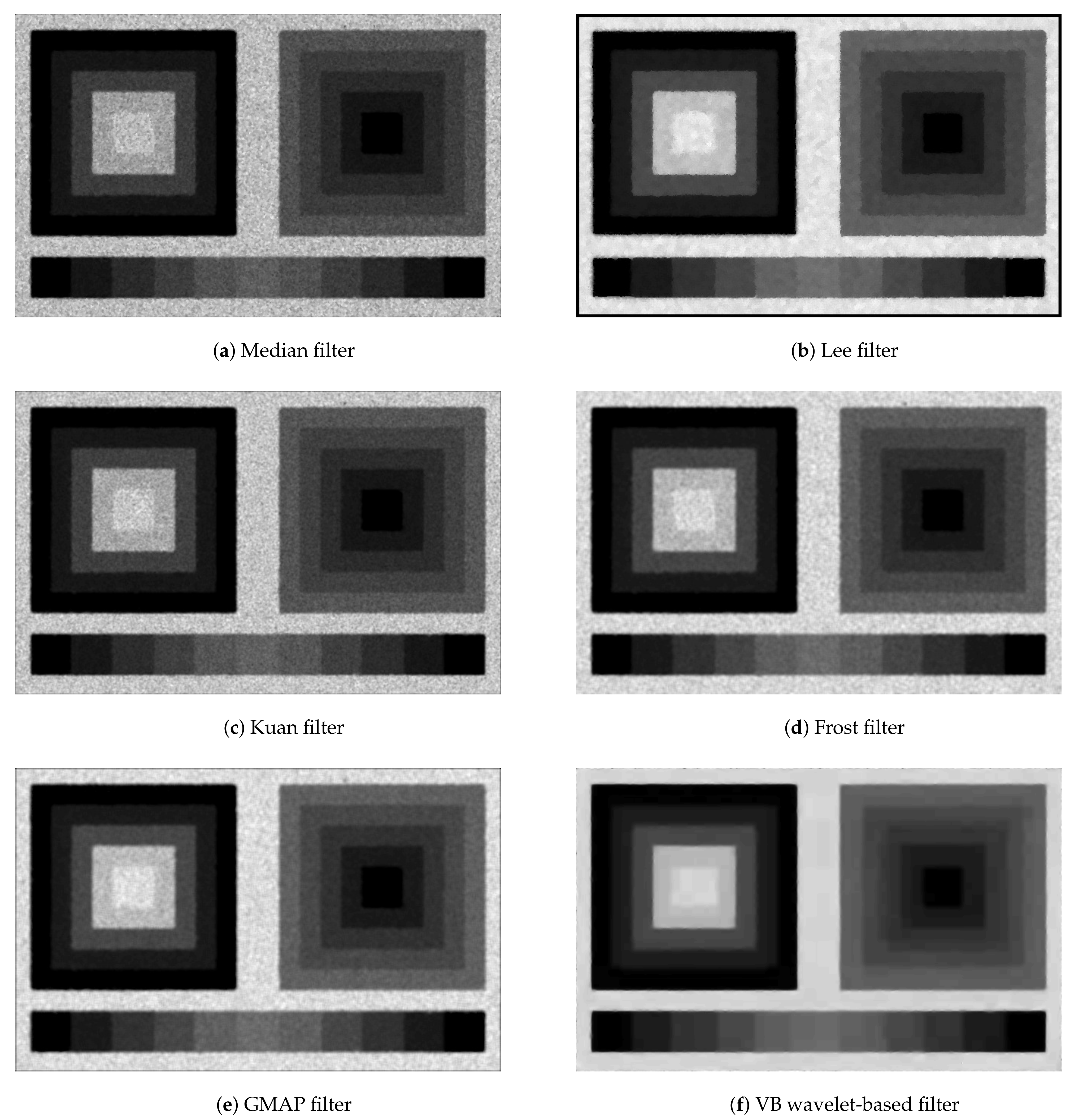
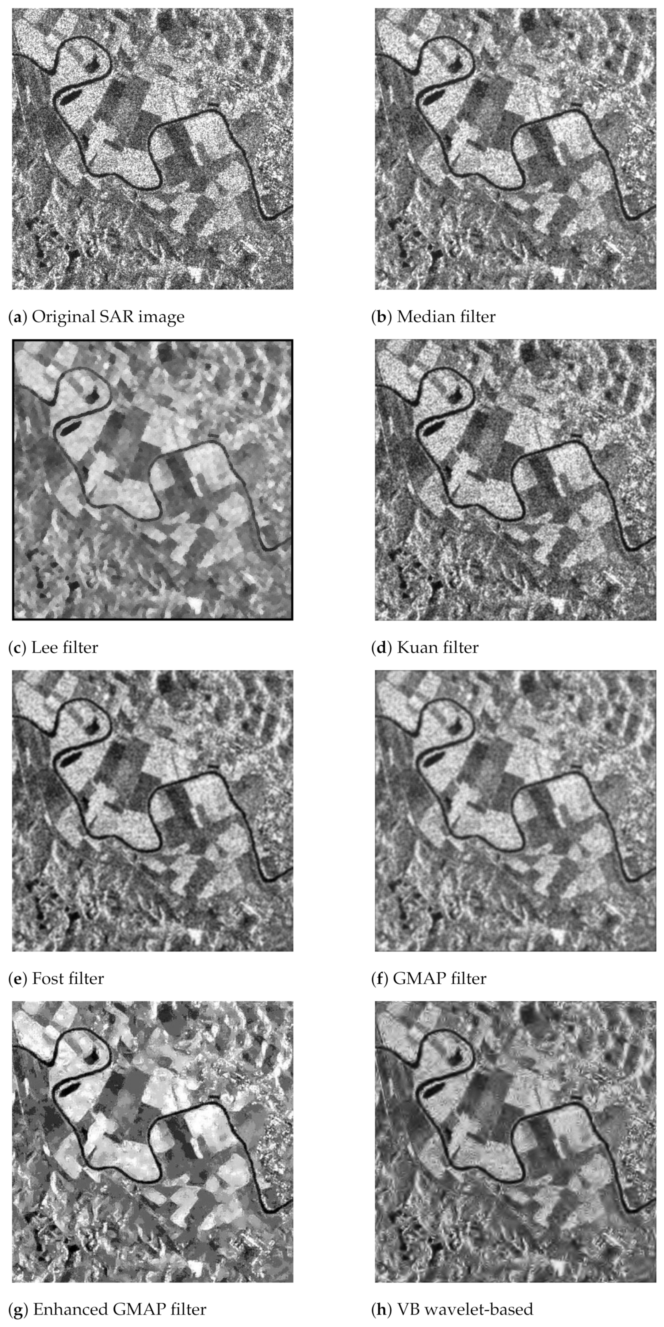
4.1.1. The Median Filter

The classical median denoising filter will be used here as the baseline method. It is a very simple algorithm, which, however, has sometimes achieved some rather impressive denoising results. This filter is non-linear, and works by moving a small image window over the original image and replacing the value of the centre pixel with the median of its neighbouring entries within the window. Note that the median is a robust measure of the central tendency of a dataset, and therefore better behaved than the mean. It’s main advantages are that, unlike some other filtering operations for speckle reduction, used for SAR multilooking, for example, the spatial resolution of filtered images using this filter is not reduced and edges are not as severely degraded and that the median filter is very efficient for filtering out salt-and-pepper type noise.

4.1.2. The Lee Filter

This filter is in a sense the prototype for all the adaptive, spatial filters in this section, which use local statistics in a moving window. Therefore some of the concepts in this subsection will be useful in other filters as well.

Starting from a signal model with multiplicative, signal dependent noise, $\mathbf{u}$, the method finds the optimal linear approximation to that observation equation such that it minimizes the mean squared error while making the model prediction an unbiased estimate of the observations [17]. The model assumes the stochastic model

$$\begin{array}{ccc}& & \mathbb{E}\left[u_n\right]={\overline{u}}_n\hfill \\ & & \mathbb{E}\left[{(u_n-{\overline{u}}_n)}^2\right]={{\sigma }_u}^2{\delta }_n{\delta }_{n^{\prime }},\hfill \end{array}$$

(45)

for the speckle noise, where ${{\sigma }_u}^2$ is its variance and $n=1,\dots ,N$ is the pixel index. These second-order statistics are approximated by the corresponding local statistics within the moving window. The resulting filtering equation is a linear filter that is exactly equivalent to a static Kalman filter, where the Kalman gain, $K_n$, serves as the signal weight, $w_n$, but with a slightly different functional form due to the approximation to the multiplicative noise. It can be shown that the Lee filter computes a weighted least-squares estimate of the despeckled signal of the form

$${\widehat{R}}_n=w_n{I}_n+\left(1-w_n\right){\overline{I}}_n,\forall n,$$

(46)

that is, it is a convex combination of the observed image, corrupted with speckle noise, $\mathbf{I}=\left(I_n\right)$, and the mean image intensity of the nth pixel’s neighbours inside the window, ${\overline{I}}_n\stackrel{\mathrm{def}}{=}\overline{{\mathbf{I}}_{\mathcal{N}\left(n\right)}}$. The weight, $w_n$, can be written in a standard form involving coefficients of variation (CV), also known as relative standard deviations (standard deviation to mean ratios), c, as

$$w_n=1-\frac{{c_u}^2}{{c_{I_n}}^2}\ge 0,$$

(47)

where

$$c_{I_n}=\frac{{\sigma }_{I_n}}{{\overline{I}}_n}\mathrm{and}{c}_u=\frac{{\sigma }_u}{\overline{u}},$$

(48)

for each pixel, n. The coefficient of variation functions as a scene texture descriptor, being a spatial heterogeneity index (SHI) of radar reflectivity in homogeneous regions.

Besides the statement of an appropriate signal model, successful despeckling, and denoising in general, hinges on the appropriate estimation of the noise level. A question then arises as to how the parameters of the speckle should be computed. The CV statistic $c_u$ can be empirically estimated by the formula $c_u=\overline{\left(\frac{\sqrt{\mathrm{Var}\left({\mathbf{I}}_h\right)}}{{\overline{I}}_h}\right)}$, where the mean and variance, ${\overline{I}}_h$ and $\mathrm{Var}\left({\mathbf{I}}_h\right)$, respectively, of the SAR image intensity are computed over a number of homogeneous areas, ${\mathbf{I}}_h$, in the image. Note that in those areas the observations are dominated by speckle. Alternatively, it can be computed by $c_u=\frac{1}{\sqrt{L}}$, where L is the effective number of looks. The last equation is notable also because it says that speckle noise drops with the square root of the number of looks, if multilook processing is chosen.

4.1.3. The Kuan Filter

The Kuan filter [18] is derived as the linear minimum mean square error (LMMSE) estimator (i.e., conditional expectation) of an additive, signal-dependent model. The filter equation is identical to the Lee filter,

$${\widehat{R}}_n=w_n{I}_n+(1-w_n){\overline{I}}_n,n=1,\dots ,N,$$

(49)

but now the weighting function, $w_n$, is

$$w_n=\frac{1-\frac{{c_u}^2}{{c_{I_n}}^2}}{1+{c_u}^2}\ge 0,$$

(50)

where, again, $c_{I_n}=\frac{{\sigma }_{I_n}}{{\overline{I}}_n}$ and $c_u=\frac{{\sigma }_u}{\overline{u}}$ are the variation coefficients of the image and noise, respectively. Note that $w_n$ is essentially a signal-to-noise ratio. The value of the Kuan-filtered image, ${\widehat{R}}_n$, is therefore a weighted avarage of $I_n$ and ${\overline{I}}_n$, the pixel’s observed grayscale value and that of the average of the pixel’s neighbourhood, with weights $w_n$ and $1-w_n$, respectively. In practice, if the value of $c_{I_n}$ falls under the noise threshold $c_u$, which means that the variation of values in the neighbourhood of pixel n is low, we assign a zero weight $w_n$ to that pixel, and, consequently, ${\widehat{R}}_n$ takes the average value in the neighbourhood.

4.1.4. The Frost Filter

Frost [19] takes a somewhat difference approach to despeckling, in that he uses a spatial autoregressive model in order to capture spatial dependencies among pixels, with a kernel (window) defined a function of the form

$$m\left(n\right)={\mathrm{e}}^{-\alpha D(n,\overline{n})},$$

(51)

where $D(n,\overline{n})$ is a distance function between the central pixel, $\overline{n}$, and a pixel beloging to the window and $\alpha$ is a damping factor. Frost, in particular, uses the weighted distance function $D(n,\overline{n})=c_{I_n}\parallel n-\overline{n}\parallel$, where $c_{I_n}=\frac{{\sigma }_{I_n}}{{\overline{I}}_n}$, as before. The Frost filtering equation is then the normalized weighted sum

$${\widehat{R}}_n=\sum _{n=1}^M\frac{m\left(n\right)I_n}{{\sum }_{n}m\left(n\right)}={\mathbf{w}}^{\mathsf{T}}{\mathbf{I}}_M,n=1,\dots ,N,$$

(52)

where M is the number of pixels within the (discrete) kernel’s spatial extent, i.e., its area of influence, and ${\mathbf{I}}_M$ denotes the vector of pixel grayscale values within the filter window.

4.1.5. The Gamma Filter

The filters discussed up to now assume either implicitly, via their use of up to second-order image statistics, or explicitly that the scene reflectivity is Gaussian-distributed. This is not a very realistic assumption, however, as reflectivity is a non-negative physical quantity. This prior knowledge can be encoded in the model using Bayesian prior probability density functions (PDFs). Lopes [20] followed this approach, and modified the Kuan LMMSE filter into a maximum a-posteriori (MAP) filter that uses non-negative, Gamma PDFs for both the noise-free scene reflectivity and the speckle noise process itself. Moreover, he proposed a more refined gradation of image texture content into three classes, homogeneous, heterogeneous, and point target, along with their corresponding thresholds. The idea behind this formulation of the filter by Lopes is to reduce speckle while retaining edges and other features of the SAR image.

Starting from the Gamma PDF (in its shape-scale parameterization [21]) for both the likelihood and the prior, solving the MAP equation,

$$\underset{\mathbf{R}}{arg\; max}\left\{log{p}_{\mathbf{u}}\left(\mathbf{u}\right)+log{p}_{\mathbf{R}\left(\mathbf{R}\right)}\right\}$$

(53)

(involving the log-posterior), and imposing the above-mentioned thresholds, one can derive the Gamma MAP (GMAP) filter

$${\widehat{R}}_n=\left\{\begin{array}{ccc}{\overline{I}}_n,\hfill & \mathrm{if}{c}_{I_n}\le c_u\hfill & \left(\mathrm{homogeneous}\right)\hfill \\ \frac{\left(\beta {\overline{I}}_n+\sqrt{\Delta }\right)}{2\alpha },\hfill & \mathrm{if}{c}_u<c_{I_n}\le c_{\max }\hfill & \left(\mathrm{heterogeneous}\right)\hfill \\ I_n,\hfill & \mathrm{if}{c}_{I_n}\ge c_{\max }\hfill & \left(\mathrm{point}\mathrm{target}\right)\hfill \end{array}\right.,$$

(54)

for each $n=1,\dots ,N$, where

$$\begin{array}{ccc}\hfill \alpha & =& \frac{1+{c_u}^2}{{c_{I_n}}^2-{c_u}^2}\hfill \end{array}$$

(55)

$$\begin{array}{ccc}\hfill \beta & =& (\alpha -L)-1\hfill \end{array}$$

(56)

$$\begin{array}{ccc}\hfill \Delta & =& {\left(\beta {\overline{I}}_n\right)}^2-4\alpha (-L{I}_n{\overline{I}}_n).\hfill \end{array}$$

(57)

Note that the CV is $c_{I_n}=\frac{\sqrt{\mathrm{Var}\left({\mathbf{I}}_M\right)}}{{\overline{I}}_n}$, and also $c_{R_n}=\sqrt{\frac{{c_{I_n}}^2-{c_u}^2}{1+{c_u}^2}}$; therefore this is also the reciprocal of the parameter $\alpha$. The thresholds in the GMAP method are given by

$$\begin{array}{ccc}\hfill c_u& =& \frac{1}{\sqrt{L}}\hfill \end{array}$$

(58)

$$\begin{array}{ccc}\hfill c_{\max }& =& \sqrt{2}{c}_u,\hfill \end{array}$$

(59)

where L is the equivalent number of looks, as before. Note that in the more complex, heterogeneous case, the MAP estimate of $R_n$ in Equation (54) is a non-linear combination of the observed intensity, $I_n$, of pixel n and the mean intensity of the neighbouring pixels of n in the window, ${\overline{I}}_n$, via the square root of discriminant $\Delta$.

4.2. Evaluation Indices

The quantitative evaluation of the studied methods will be performed via the use of a number of indices, some of which are generic and others specific for speckle. The former include:

• The Pearson correlation coefficient (corrcoef), $r\left(\widehat{\mathbf{x}},\mathbf{x}\right)$,

  $$r\left(\widehat{\mathbf{x}},\mathbf{x}\right)=\frac{{\sum }_n(x_n-\overline{x})({\widehat{x}}_n-\widehat{\overline{x}})}{\sqrt{{\sum }_n{(x_n-\overline{x})}^2}\sqrt{{\sum }_n{({\widehat{x}}_n-\widehat{\overline{x}})}^2}},$$

  (60)

  where $\widehat{\mathbf{x}}$ is a model estimate of a (known, in this case) quantity, $\mathbf{x}$.
• The signal-to-noise ratio (SNR), measured in dB,

  $$\mathrm{SNR}=10{log}_{10}\left(\frac{\mathbb{E}\left[{\mathbf{x}}^2\right]}{\mathbb{E}\left[{\epsilon }^2\right]}\right),$$

  (61)

  where $\widehat{\epsilon }=\mathbf{x}-\widehat{\mathbf{x}}$ is the error committed by the estimator at hand, leading to the mean squared error (MSE), where $\mathrm{MSE}=\frac{1}{N}{\sum }_{n=1}^N{{\epsilon }_n}^2$.
• The peak signal-to-noise ratio (PSNR), measured in dB,

  $$\mathrm{PSNR}=10{log}_{10}\left(\frac{{{\max }_{\mathbf{x}}}^2}{\mathrm{MSE}}\right),$$

  (62)

  where ${\max }_{\mathbf{x}}$ is the maximum grayscale value an image can take, e.g., $2^8-1$ for an 8–bit encoded image.

The latter are without–reference indices, that is, they only operate on pairs of observed and reconstructed images, without the need for ground truth. These are essential for assessing the quality of reconstruction of real-world images [22]. These include:

• The Equivalent Number of Looks (ENL). ENL, which is a measure of noise level, is one of the most common indices used in SAR images. It is defined as

  $$\mathrm{ENL}=\tilde{L}=\frac{\mathbb{E}{\left[\mathbf{I}\right]}^2}{\mathrm{Var}\left[\mathbf{I}\right]}.$$

  (63)
  ENL refers to one image, and can be used both on the original, observed image and the reconstructed image. In multilook processing, the number of looks, L, of a SAR image is the number of independent images of a scene that have been averaged to produce a smoother image, and, as mentioned before, speckle noise drops by the square root of L. In the case of a single image, the equivalent number of looks, $\tilde{L}$, is a good measure of the speckle noise level. To compute the ENL, one selects a large uniform image region, or a number of such regions, and computes the empirical statistics of speckle there.
• The Edge Preserving Index (EPI), as the name implies, is a measure of the edge and linear feature preserving capability of despeckling algorithms. Since any form of denoising inevitably leads to some degradation of high-frequency features, this is an important quality index in SAR. EPI therefore compares the edges of the original with those of the restored image, and is computed as the ratio of highpass versions of the original and despeckled images. A simple definition is

  $$\mathrm{EPI}=\frac{{\sum }_{ij}|{\widehat{R}}_{i+1,j}-{\widehat{R}}_{i,j}|+|{\widehat{R}}_{i,j+1}-{\widehat{R}}_{i,j}|}{{\sum }_{ij}|I_{i+1,j}-I_{i,j}|+|I_{i,j+1}-I_{i,j}|},$$

  (64)

  where the pixel indices $ij$ were used here to highlight the row-wise and column-wise operations, respectively. In practice, smoother forms of edge detection may be used, for example using a higher-order Laplacian filter, implementing the operator

  $$\Delta f(x,y)=\frac{{\partial }^{2}f(x,y)}{\partial x^2}+\frac{{\partial }^{2}f(x,y)}{\partial y^2}.$$

  (65)
  From its functional form it is easy to see that EPI is analogous to an edge correlation index. A value of one indicates perfect edge preservation. The SNR and corrcoef are measures that use global image properties. On the contrary, oftentimes we want to focus on specific features, such as edges. EPI complements those measures.
• The Radiation Accuracy Error (RAE) is a measure of radiometric loss due to filtering between the original image and the filtered image. It therefore operates on the pair of original and filtered images and is defined as the ratio of the average grayscale values of the estimated SAR image to that of the measured one:

  $$\mathrm{RAE}=10{log}_{10}\left(\frac{\mathbb{E}\left[\widehat{\mathbf{R}}\right]}{\mathbb{E}\left[\mathbf{I}\right]}\right),$$

  (66)
  A value close to zero indicates an unbiased estimator.

5. Experiments and Analysis

In this section, experiments on simulated data and real SAR images are described. A comparison study between our method and the major filters used for speckle reduction in practice, given in Section 4.1, was performed and the results were evaluated perceptually and numerically. For our variational Bayesian wavelet-based method, the classical Symlet 8 wavelet family was used in all experiments, as it provides a good balance between frequency and time resolution, and has been widely used in image processing research, without being specialized to any particular image. The various evaluation indices that were used are given in Section 4.2.

First, the experimental results of applying the above methods and the proposed one on these datasets are presented, and then a critical analysis of the pros and cons of the most competitive filter and our proposed method as well as some pointers for future research are given.

5.1. Experiments with Simulated SAR Images

To test the speckle reduction abilities of our method, and to compare it with established algorithms, we performed a simulation study, inspired by a similar study by Sun et al. [22]. Simulated SAR images were created by adding multiplicative noise to a known ‘clean’ target image. Two noise levels, of $20\%$ and $50\%$ noise with respect to the signal, were used. Examples of those images are shown in Figure 5.

We ran the various established speckle reduction filters discussed in Section 4.1 and our own proposed method (Section 2) on this dataset and evaluated the results using the despeckling performance indices presented in Section 4.2. For comparison, we present the resulting denoised images arranged together, per noise level, in the order the filters were introduced, except for our own method which will be presented last. Figure 6 displays the results for the simulated images corrupted with $20\%$ noise, and Figure 7 the corresponding results for the $50\%$ noise. The numerical evaluation indices for the corresponding methods, and for the two noise levels, are shown in

Table 1. Evaluation indices for the SAR speckle reduction simulation experiment at 20% noise level, for the various methods examined in this paper. The corresponding despeckled images are displayed in Figure 6. The best result for each index is marked in bold typeface.

	Corr. Coef.	SNR (dB)	PSNR (dB)	ENL	EPI	RAE
Median filter	0.9950	12.171	28.907	57.565	0.7500	−0.013079
Lee filter	0.8734	5.1333	14.831	84.751	0.3985	−0.2191
Kuan filter	0.9935	11.593	27.750	50.878	0.5680	−0.025053
Frost filter	0.9974	13.566	31.696	157.22	0.9427	−7.8217$\times {10}^{-3}$
GMAP filter	0.9911	10.856	26.277	63.864	0.7497	−0.051018
VB Wavelets	0.9990	15.384	35.332	633.14	0.9720	1.3528$\mathbf{\times }{\mathbf{10}}^{-\mathbf{4}}$

and

Table 2. Evaluation indices for the SAR speckle reduction simulation experiment at 50% noise level, for the various methods examined in this paper. The corresponding despeckled images are displayed in Figure 7. The best result for each index is marked in bold typeface.

	Corr. Coef.	SNR (dB)	PSNR (dB)	ENL	EPI	RAE
Median filter	0.9890	10.431	25.427	31.717	0.5621	−0.023736
Lee filter	0.8723	5.1149	14.794	57.672	0.3222	−0.2188
Kuan filter	0.9898	10.625	25.814	34.399	0.4656	−0.027765
Frost filter	0.9960	12.643	29.850	85.742	0.9225	−8.1316$\times {10}^{-3}$
GMAP filter	0.9899	10.598	25.760	46.723	0.6776	−0.049878
VB Wavelets	0.9980	13.753	32.071	276.57	0.9560	5.8928$\mathbf{\times }{\mathbf{10}}^{\mathbf{-}\mathbf{4}}$

, respectively.

As a general comment, we first note that the descpeckling capabilities of the filters were consistent, that is their relative ranking did not change (the worst filter remained worst, and analogously for the others) with respect to the noise level. All methods achieved a very high correlation coefficient (above $0.99$), except for the Lee filter. However, observing the resulting images, it becomes obvious that there were important differences with respect to how well the various methods did. (This leads to the conclusion that, while the correlation coefficient was a useful indicator of the overall performance of a method, this index should always be interpreted in combination with the other evaluation indices.) Except for the Lee filter, and to some degree the Kuan filter, all the others managed to maintain edges pretty well. This was reflected in their EPI index, which was around and above $0.7$ in most cases. Visually, the ranking of the methods studied in terms of speckle reduction, from best to worst, is VB wavelet-based method, Frost filter, GMAP filter, Lee filter, Kuan filter, Median filter.

In particular, the median filter did not perform very well for this task, in both cases. A large percentage of speckle noise in the simulated SAR images remained. The Kuan filter did somewhat better than the median filter, as it discriminated homogeneous areas of different grayscale texture slightly better, but it was still quite noisy. The Lee filter did reasonably well for this task, but it introduced considerable blurring in the results. As a consequence, edges in the image became smeared. Interestingly, the addition of significantly more speckle in the second noise regime did not seem to have a severe effect on the results of this filter. The Gamma MAP filter did somewhat worse than expected, given its strong theoretical foundation. Although it visually produced slightly brighter images than the Frost filter, all its evaluation indices were significantly worse than those of the Frost filter, except for the correlation coefficient. This radiometric difference was however artificial, since the radiation accuracy error (RAE) of the Frost filter was almost an order of magnitude better than that of the Gamma MAP. This behaviour seemed to repeat over the experiments. Conversely, the Frost filter performed surprising well for this task, with all its evaluation scores being significantly higher than all the other established methods studied. We attribute this performance to its use of a proper distance kernel, which seemed to weight each individual pixel contribution in its area of influence better than the simple average of the other filters. It also performed very well with respect to edge preservation for this task. The variational Bayesian wavelet-based method performed the best, managing to reduce speckle almost perfectly for this task, and also in terms of edge preservation. This is reflected in its quantitative evaluation scores over all indices (Table 1 and Table 2), which were significantly higher than all the competing methods. In particular, its equivalent number of looks (ENL) and radiation accuracy error (RAE) scores were an order of magnitude better than those of the other methods, while the SNR and PSNR achieved a double score (logarithmic scale) and the edge preservation index (EPI) was almost 1.

5.2. Despeckling of Real SAR Images

In this section we will demonstrate the performance of our variational Bayesian wavelet-based denoising method on a real SAR image acquired by the ERS 1 satellite (Images or videos released by ESA under Creative Commons Attribution-ShareAlike 3.0 IGO (CC BY-SA 3.0 IGO) Licence, https://www.esa.int/ESA_Multimedia/Copyright_Notice_Images (accessed on 3 June 2021)) [23], over Tiber Valley north to Rome, Italy, on 21 April 1994 (Figure 8).

The image shows some agricultural fields located along the river Tiber and some hilly areas. This image was chosen for two reasons: first, older SAR images are ideal for demonstrating despeckling algorithms, as they are more heavily impacted by noise, while providing an invaluable resource for multi-temporal analysis, and second, as a means for comparison with established, as well as more state-of-the-art denoising algorithms. Regarding the latter, more refined reconstruction techniques can be defined, such as combining speckle filtering with edge and line detection algorithms. One such reconstruction method, of particular interest for the reasons explained below, will be given later in this section.

We applied the previously presented despeckling algorithms, Median, Lee, Kuan, Frost, Gamma MAP, and our variational Bayesian wavelet-based method, along with an enhanced version of Gamma MAP, employing edge and line detection. This section is structured in two parts. We first give a qualitative, visual assessment of the results and link those aspects of the evaluation to the corresponding numerical indices, presented in

Table 3. Evaluation indices ENL, EPI, and RAE for the real, Tiber Valley SAR image reconstructions from each of the despeckling methods examined (see text for explanation). The best result for each index is marked in bold typeface.

	ENL	EPI	RAE
Median filter	14.280	0.6333	0.029565
Lee filter	32.158	0.5156	−0.073089
Kuan filter	17.112	0.6340	−0.011139
Frost filter	27.402	0.5144	−5.0381$\times {10}^{-3}$
Gamma MAP filter	28.623	0.6197	−0.020175
Enhanced Gamma MAP	47.294	0.5561	0.1333
VB Wavelet Method	55.696	0.6648	6.7503$\mathbf{\times }{\mathbf{10}}^{\mathbf{-}\mathbf{14}}$

. In particular, we used the without–reference evaluation indices ENL, EPI, and RAE; in real-world data we do not have the actual scene reflectivities to compared to. (In the Inverse Problems and Machine Learning terminology, this is a blind image reconstruction problem.) According to our analysis below, these indices managed to capture the essential aspects of despeckling performance on real-world SAR images. We then give a more analytical comparison of the most competitive result to the proposed method, emphasizing their pros and cons.

We show the collective results in Figure 9, side-by-side, to make comparison easier, and we we comment on each method and its corresponding resulting image.

As mentioned above, the Median filter was used here as the baseline method. It did not manage to adequately despeckle the image in this case, as displayed in Figure 9b, which resulted in the lowest equivalent number of looks (ENL). However, its edge preserving index (EPI) was quite high. This apparent contradiction was resolved by reflecting on what the EPI computed. In essence, it was a measure of similarity between the observed noisy image and the denoised one. While its focus is on revealing how much the edges and other features were preserved during despeckling, its domain was over the whole image. Comparing the Median-despeckled image with the original observations, we realize that the filter did not alter the observed data enough, hence the relatively high EPI.

The established algorithms used for SAR despeckling (Lee, Kuan, Frost, and Gamma MAP) performed sufficiently well in this task, as expected, but with some variability in the results. The Lee algorithm, however, produced overblurred results (Figure 9c), which is something that was reflected in its ENL index, and it was not very good at preserving detail, as is reflected in its EPI index, which was the second lowest of the algorithms studied. We believe that the blurring stems from the nature of the basic algorithm, as essentially an optimal linear filter that assumes Gaussian statistics, which does not represent a physically plausible condition.

Similarly to the Median filter, the Kuan filter (Figure 9d) was also somewhat noisy, and with a very similar EPI, while achieving a slightly higher ENL. However, it also produced slightly darker images than the Median filter.

The Fost filter achieved somewhat better denoising results, but it was quite bad at preserving detail, as it is reflected in its EPI index, which was the lowest of the algorithms studied (Figure 9e). We can attribute its relative efficiency to the particular form of kernel that the method used. Nevertheless, its speckle suppression performance for this task was still mediocre. The kernel could potentially be refined and fine-tuned; however, the method still assumed a Gaussian distribution for the image statistics. Therefore, it is unclear how far this method could be pushed in order to achieve state-of-the-art results.

All of the above despeckling methods achieved a RAE index of a similar order (${10}^{-2}$), preserving the original SAR image radiometry.

The Gamma MAP filter produced the best results out of the established despeckling algorithms for this task. It was more balanced than the previous filters, providing the cleanest results of this group and preserving image detail relatively well. The despeckling result of this filter is shown in Figure 9f. We can attribute this mostly to the use of a proper, non-negative, Gamma prior for the noise-free scene and the speckle noise. However, some of the details, especially the finer ones, were still not preserved well. In fact the Gamma MAP filter achieved an edge preserving index lower that that of the Median and the Kuan filter.

As mentioned above, an interesting approach is the combination of despeckling filters with other methods, e.g., feature extraction. One such reconstruction, using an enhanced Gamma Map filter, is shown in Figure 9g, from the ESA site [24] (ESA did not give the particular details of the implementation of this filter). This combination produced the most competitive results to our proposed method in terms of visual appearance, at least. It achieved an estimated equivalent number of looks much higher than the standard despeckling methods; however both its EPI and RAE indices were rather mediocre. In particular, they were lower than those of the standard Gamma MAP filter. This implies a better denoising/smoothing but a not-so-good edge and radiometry preservation. We will investigate this issue further below, after we first present the results of our proposed method and comment on the indicators a little more thoroughly.

Our Bayesian wavelet-based method performed very well on this task, displaying very good capability for speckle suppression while retaining edges and shape features in the image (Figure 9h); this is reflected in all its numerical evaluation indices, shown in Table 3, which were the best among all competing methods. The nature and possible cause of some artifacts that seemed to be remaining and possible ways to fix them will be discussed below.

The numerical comparison of the various despeckling methods examined in this paper with respect to this image is summarized in Table 3.

Let us analyze these results in more detail. First, we note that the methods have been arranged with respect to their mathematical sophistication and evolution of development (first column), as discussed above. In addition, we should stress that the above evaluation metrics should be interpreted in combination, since they emphasize different aspects of image reconstruction, in order to illuminate insights: it may look surprising at first that some simple methods, such as the Median filter, for example, achieve better scores for some indices than the much more sophisticated Modified Gamma MAP filter, if taken individually. However, even a simple visual inspection shows that the Median filter does not perform so well in this task. This can be quantified by the crucial ENL metric. The combination of the three metrics can give us a more fine-grained, quantitative comparison among methods that look qualitatively similar. Nevertheless, if an image analyst wants to emphasize a particular aspect of a method, such as edge preservation, for example, then a focus on a particular metric might be appropriate. As in all inverse problems, the particular task at hand should inform the particular strategy one should follow.

We are now in a position to make a more informed evaluation of the two best results. Going back to the enhanced Gamma MAP filter (Figure 9), we note that it seemed to produce slightly cartoonish images, giving it a look reminiscent of an oil painting, which, while æsthetically pleasing, do not seem very realistic for SAR. In that respect it was somewhat similar to the result produced by the Lee filter. Additionally, notice that the despeckled image looked brighter than the original; this is because the RAE index was positive and relatively large. The method therefore was not unbiased, in the statistical sense (a perfect RAE index should be zero). Comparing equivalent areas of the original SAR image and the one produced by the Enhanced Gamma MAP filter, for example the upper-left part, we see that that algorithm artificially tinted parts of the image. Indeed, the above can be quantified by the fact that all evaluation indices, ENL, EPI, and RAE, were significantly lower than those produced by our method.

Close inspection shows that our method managed to preserve edges and linear features better than the Enhanced Gamma MAP filter. This was reflected in the much higher EPI measure. It seems that the Enhanced Gamma MAP filter oversmoothed the image, losing some significant details. Overall, our method achieved significantly higher scores over all evaluation metrics. Nevertheless, our method still contained some artifacts, in particular in areas of homogeneous texture. Focusing on those areas and closely examining the shape and orientation of those artifacts reveals that this is most likely a result of the current use of the particular wavelet basis, which was not rotationally invariant. This means that these bases, taken individually, did not describe those particular features optimally, and a destructive interference of a number of those bases was needed to locally produce a result similar to that of the Enhanced Gamma MAP filter in these areas. However, the combination with the global search for sparsity, seemed to disallow this effect. However, there are a variety of other, wavelet-like bases, such as curvelets, ridgelets and bandelets, which possess this property and could be used in the future. For example, Argenti and Alparone [25] present one such choice, using the undecimated wavelet transform. Kseneman and Gleich [26] use second generation wavelets, in particular bandelets and contourlets, under a maximum a-posteriori (MAP) framework, with very promising results. In this paper, the emphasis was on providing the fully Bayesian, variational inference scheme. The combination of these more adapted local image bases with our variational Bayesian framework is a topic of ongoing research.

6. Conclusions

We introduced a fully Bayesian, variational framework for inference and learning under uncertainty, and applied the method to a constrained version of the general Gaussian mixture model specifically tailored to model sparse sets of decomposition coefficients, such as those obtained from wavelet-type decompositions of signals. Modelling those coefficients under a mean-field approximation allows an efficient algorithm to be derived. The general derivation of the equations of variational inference was shown, connections with relevant Statistical Physics concepts was given, and then the specific update equations and negative free energy functional for the SMoG model were derived in the context of Bayesian networks. Particular emphasis was given to the locality of computations offered by the structuring of sets of random variables in a DAG with probabilistic semantics.

The sparse representation model and learning algorithm was then used to infer the wavelet decomposition coefficients of SAR images and other remotely-sensed Earth signals, with the particular aim of developing a denoising scheme for those signals. The corresponding processor formulated in the above efficient variational framework avoids costly sampling methods such as Markov chain Monte Carlo, and employs a flexible prior per decomposition scale whose posterior hyperparameters are learned directly from the data and adapt to the characteristics of the particular dataset at hand.

We applied the model to both synthetic data and real SAR images and evaluated the results using standard quality metrics for SAR denoising. The results show that our algorithm is more effective than traditional despeckling methods both in terms of speckle reduction and preservation is image details such as edges.

In this work we used the generic, ‘least asymmetric’, orthogonal wavelet family, since we focused more on the theoretical foundation and proof of concept. This is very efficient for sparsity but it can be suboptimal for pattern representation and recognition. Future work will refine and extend the method to more effective families, and possibly take into account residual dependencies among representation coefficients. Another avenue for research is the combination of pure denoising/despeckling with other image processing operations, such as edge and line detection algorithms, and the investigation of the effect of our method on subsequent processing for SAR interferometry and polarimetry. A comparison with Markov Chain Monte Carlo using Gibbs sampling (which provides somewhat similar expressions and piecemeal update philosophy but approaching the problem from a stochastic simulation viewpoint), in terms of quality of results and running time with experimental data, is a topic of ongoing research.

References

1. Olshausen, B.A.; Millman, K.J. Learning Sparse Codes with a Mixture-of-Gaussians Prior. In Advances in Neural Information Processing Systems 12; Solla, S.A., Leen, T.K., Müller, K., Eds.; MIT Press: Cambridge, MA, USA, 2000; pp. 841–847. [Google Scholar]
2. Roussos, E.; Roberts, S.; Daubechies, I. Variational Bayesian Learning for Wavelet Independent Component Analysis. In Proceedings of the 25th International Workshop on Bayesian Inference and Maximum Entropy Methods in Science and Engineering, San Jose, CA, USA, 7–12 August 2005; AIP: New York, NY, USA, 2005. [Google Scholar]
3. Bernardo, J.M.; Smith, A.F.M. Bayesian Theory; Wiley: Hoboken, NJ, USA, 2000; p. 610. [Google Scholar]
4. Attias, H. A Variational Bayesian Framework for Graphical Models. In Advances in Neural Information Processing Systems 12; MIT Press: Cambridge, MA, USA, 2000; pp. 209–215. [Google Scholar]
5. Beal, M.J.; Ghahramani, Z. Variational Bayesian learning of directed graphical models with hidden variables. Bayesian Anal. 2006, 1, 793–831. [Google Scholar] [CrossRef]
6. Frigyik, B.A.; Kapila, A.; Gupta, M.R. Introduction to the Dirichlet Distribution and Related Processes; Technical Report UWEETR-2010-0006; Department of Electrical Engineering, University of Washington: Seattle, WA, USA, 2010. [Google Scholar]
7. Gelman, A. Prior distributions for variance parameters in hierarchical models. Bayesian Anal. 2006, 1, 515–534. [Google Scholar] [CrossRef]
8. Gelfand, I.M.; Fomin, S.V. Calculus of Variations; Prentice Hall: Englewood Cliffs, NJ, USA, 1963; p. 240. [Google Scholar]
9. Bishop, C.M. Neural Networks for Pattern Recognition; Oxford University Press Inc.: New York, NY, USA, 1995; p. 482. [Google Scholar]
10. Penny, W.; Roberts, S. Variational Bayes for 1-Dimensional Mixture Models; Technical Report PARG–00–2; Department of Engineering Science, University of Oxford: Oxford, UK, 2000. [Google Scholar]
11. Dempster, A.P.; Laird, N.M.; Rubin, D.B. Maximum Likelihood from Incomplete Data via the EM Algorithm. J. R. Stat. Soc. Ser. B (Methodol.) 1977, 39, 1–38. [Google Scholar]
12. Coggeshall, F. The Arithmetic, Geometric, and Harmonic Means. Q. J. Econ. 1886, 1, 83–86. [Google Scholar] [CrossRef]
13. Choudrey, R. Variational Methods for Bayesian Independent Component Analysis. Ph.D. Thesis, Department of Engineering Science, University of Oxford, Oxford, UK, 2003. [Google Scholar]
14. Mallat, S. A Wavelet Tour of Signal Processing, 3rd ed.; Academic Press: Cambridge, MA, USA, 2008. [Google Scholar]
15. Huang, S.Q.; Liu, D.Z. Some uncertain factor analysis and improvement in spaceborne synthetic aperture radar imaging. Signal Process. 2007, 87, 3202–3217. [Google Scholar] [CrossRef]
16. Argenti, F.; Lapini, A.; Bianchi, T.; Alparone, L. A Tutorial on Speckle Reduction in Synthetic Aperture Radar Images. IEEE Geosci. Remote Sens. Mag. 2013, 1, 6–35. [Google Scholar] [CrossRef] [Green Version]
17. Lee, J.S. Digital image enhancement and noise filtering by use oflocal statistics. IEEE Trans. Pattern Anal. Mach. Intell. 1980, 2, 165–168. [Google Scholar] [CrossRef] [PubMed] [Green Version]
18. Kuan, D.T.; Sawchuk, A.A.; Strand, T.C.; Chavel, P. Adaptive noise smoothing filter for images with signal-dependent noise. IEEE Trans. Pattern Anal. Mach. Intell. 1985, 7, 165–177. [Google Scholar] [CrossRef] [PubMed]
19. Frost, V.S.; Stiles, J.A.; Shanmugan, K.S.; Holtzman, J.C. A Model for Radar Images and Its Application to Adaptive Digital Filtering of Multiplicative Noise. IEEE Trans. Pattern Anal. Mach. Intell. 1982, 4, 157–166. [Google Scholar] [CrossRef] [PubMed]
20. Lopes, A.; Nezry, E.; Touzi, R.; Laur, H. Structure detection and statistical adaptive speckle filtering in SAR images. Int. J. Remote Sens. 1993, 14, 1735–1758. [Google Scholar] [CrossRef]
21. Bernardo, J.M.; Smith, A.F.M. Bayesian Theory; John Wiley & Sons: New York, NY, USA, 1994. [Google Scholar]
22. Sun, B.; Chen, J.; Tovar, E.J.; Qiao, Z.G. Unbiased-average minimum biased diffusion speckle denoising approach for synthetic aperture radar images. J. Appl. Remote Sens. 2015, 9, 1–13. [Google Scholar] [CrossRef] [Green Version]
23. ESA Earth Online, Radar Course. Available online: https://earth.esa.int/web/guest/missions/esa-operational-eo-missions/ers/instruments/sar/applications/radar-courses/course-3 (accessed on 30 May 2021).
24. Image Interpretation. Available online: https://earth.esa.int/web/guest/missions/esa-operational-eo-missions/ers/instruments/sar/applications/radar-courses/content-3/-/asset_publisher/mQ9R7ZVkKg5P/content/radar-course-3-image-interpretation-tone (accessed on 20 November 2019).
25. Argenti, F.; Alparone, L. Speckle Removal from SAR Images in the Undecimated Wavelet Domain. IEEE Trans. Geosci. Remote Sens. 2002, 40, 2363–2374. [Google Scholar] [CrossRef]
26. Kseneman, M.; Gleich, D. Information Extraction and Despeckling of SAR Images with Second Generation of Wavelet Transform; Advances in Wavelet Theory and Their Applications in Engineering, Physics and Technology; IntechOpen: Rijeka, Croatia, 2012. [Google Scholar] [CrossRef] [Green Version]
Figure 1. Sparse mixture of Gaussians (SMoG) density, here used as an adaptive prior for the decomposition coefficients, { c λ } , of a sparse signal. Blue/green curves: Gaussian components; thick black curve, mixture density, p ( c λ ) . In multiscale, wavelet-type analysis, a separate SMoG is placed on each dyadic scale.
Mca 26 00045 g001
Figure 2. Bayesian network representation, G SMoG , of a sparse mixture of Gaussian (SMoG) density. Brown rectangles represent ‘plates’, iterating over collections of variables. The plate over n represents the collection ( y n , ξ n ) , n = 1 , , N , of pairs of state and representation coefficient values, for each data point n. The plates over m represent the parameters of the set of M Gaussian components, Θ SMoG = μ m , β m π , m = 1 , , M , stored in a vector θ SMoG . These collectively model the generally non-Gaussian density of the coefficients of a signal. Filled nodes, such as y n , denote instantiated nodes. Rectangle nodes denote hyperparameters of the model. In multiscale, wavelet-type analysis this DAG is replicated for each dyadic scale, j, as well, resulting in a collection of parameters, Θ SMoG = j Θ SMoG j .
Mca 26 00045 g002
Figure 3. The negative free energy (NFE), F q , forms a lower bound to the Bayesian log-evidence for a data set under the model, log p Y . Their difference is the Kullback–Leibler divergence, KL q p , between the variational posterior, q ( U ) , and the true posterior, p ( U | Y ) . The NFE is the optimization function of the VB methodology.
Mca 26 00045 g003
Figure 4. Detection of transient signals in noisy Geodetic time series. Blue line: annual and semiannual harmonic signals. Brown line: transient signal. Gray dots: a mixture of white noise as well as coloured noise. Lower panel: green line: original signal, red line: reconstruction by the algorithm.
Mca 26 00045 g004
Figure 5. Instances of simulated SAR images for assessing the speckle reduction methods used in this paper. (a) 20% noise. (b) 50% noise. Adapted from Sun et al. [22], under the Attribution 3.0 Unported (CC BY 3.0) licence. ‘Clean’ targets were cropped from the original and simulated speckle was added.
Mca 26 00045 g005
Figure 6. Speckle reduction simulation experiment at 20% noise level. The reconstructed images are arranged according to the filters Median, Lee, Kuan, Frost, Gamma MAP, and, finally, our VB wavelet-based method. The corresponding numerical evaluation indices are shown in Table 1.
Mca 26 00045 g006
Figure 7. Speckle reduction simulation experiment at 50% noise level. The reconstructed images are arranged according to the filters Median, Lee, Kuan, Frost, Gamma MAP, and, finally, our VB wavelet-based method. The corresponding numerical evaluation indices are shown in Table 2.
Mca 26 00045 g007
Figure 8. The original ERS 1 SAR image of Tiber Valley (Central Italy). (Image: ESA).
Mca 26 00045 g008
Figure 9. Aggregated results of all despeckling methods examined in this paper on the noisy ERS 1 SAR image of Tiber Valley (Central Italy) of Figure 8. See text and individual images for an analysis of the results.
Mca 26 00045 g009