Article

Operational Risk Reverse Stress Testing: Optimal Solutions

Department of Computer Science, University College London, Gower Street, London WC1E 6BT, UK
Math. Comput. Appl. 2021, 26(2), 38; https://doi.org/10.3390/mca26020038
Submission received: 24 March 2021 / Revised: 19 April 2021 / Accepted: 26 April 2021 / Published: 28 April 2021

Abstract

:
Selecting a suitable method to solve a black-box optimization problem that uses noisy data was considered. A targeted stop condition for the function to be optimized, implemented as a stochastic algorithm, makes established Bayesian methods inadmissible. A simple modification was proposed and shown to improve optimization the efficiency considerably. The optimization effectiveness was measured in terms of the mean and standard deviation of the number of function evaluations required to achieve the target. Comparisons with alternative methods showed that the modified Bayesian method and binary search were both performant, but in different ways. In a sequence of identical runs, the former had a lower expected value for the number of runs needed to find an optimal value. The latter had a lower standard deviation for the same sequence of runs. Additionally, we suggested a way to find an approximate solution to the same problem using symbolic computation. Faster results could be obtained at the expense of some impaired accuracy and increased memory requirements.

1. Introduction

Reverse Stress Testing (RST) is a relatively new technique for finding cases that cause a bank to cross the barrier between survival and default. Bank default can lead to a chain of further defaults, so determining how RST should be done is vital for limiting systemic risk. Stress testing, in which outcomes resulting from amended model parameters are calculated, is more common and is a regulatory requirement. The precise distinction between reverse stress testing and stress testing is discussed in Section 2. In this paper, we suggest an optimal way to do RST in the context of operational risk, which is the risk of incurring financial loss from adverse events. In doing so, we make a significant improvement to an established optimization method and provide evidence that our suggestion is, indeed, optimal. Sufficient guidance for practitioners is given to enable sufficiently accuracy to be achieved.
We considered the problem of optimizing a real-valued black-box function f ( D , x ) of data, D, where x is a parameter value to be optimised. The domain of x is a closed real interval I. Function f is a Value-at-Risk (VaR) calculator, which incorporates a non-linear Monte Carlo process that is subject to significant stochastic variation. Consequently, the VaR calculation takes excessive time to evaluate if too many Monte Carlo cycles are used. Too many evaluations would be procedurally intractable. We call such functions “expensive”. An optimization method that minimises two factors is therefore required. In a sequence of independent runs under precisely the same conditions, the first factor is the mean number of runs required to complete the optimization. The second factor is the corresponding standard deviation.

1.1. The Context: Operational Risk and Stress Testing

Every year, financial institutions (banks, insurance companies, pension funds, etc.) have to demonstrate that they are resilient to adverse economic conditions. To do that, they are required to calculate, using an appropriate model, what level of capital reserves would be necessary for the upcoming year. The most common type of stress test is to amend either model parameters, or to amend data, re-run the model and assess the outputs in light of the amended inputs. There are often correlations between operational risk and economic factors, but such correlations are also often weak or absent completely. The subject was touched upon in [1], where a much more robust method of stress testing was presented. In RST, a desired level of stress in VaR is decided in advance, and the necessary data and/or parameter changes to achieve that stress level are calculated. Further details are in Section 2.
The context considered in this paper is operational risk, which arises from adverse events that result in monetary loss. Operational risk may be summarised in the following definition from the Bank for International Settlements (BIS) [2]:
       "The risk of loss resulting from inadequate or failed
     internal processes, people and systems or from external events"
Operational risk losses are payments related to non-financial adverse events (as opposed to financial events in credit and market risk). They may be characterised by the “Five-Fs”:
             Fails Fire Flood Fines Fraud
One further category—Conduct–is not represented in the “Five-Fs”’ list. Conduct risk losses subsume the fines category and tend to be treated separately from others because conduct risk loss distributions are often heavily skewed by a huge single loss (possibly hundreds of million euros). Other operational risk losses range from very small (10 euros) to a few million euros and usually fit a fat-failed distribution (such as log normal). Some examples from the data used in this study are (all in £ sterling):
  • 140: ex gratia payment;
  • 18,000: damage to a bank branch caused during a robbery;
  • 187,000: computer hacking fraud;
  • 42,000,000: provision for mis-selling.
A notable operational risk loss appeared at the end of 2020: customer compensations for fraud as a result of the 2020 COVID-19 pandemic. They amounted to £10.88m, although that figure came too late for inclusion in the data for this study.
Operational risk reserves are usually calculated in terms of the 99.9% Value-at-Risk (VaR, using the Loss Distribution Approach (LDA) algorithm of Frachot et al. [3]. The 99.9% quantile is specified in the BIS regulations [4]. The LDA algorithm is summarised in Appendix A, where implementations in R and Mathematica are also shown. Steps marked (**) are used in Section 5.

1.2. Contribution of this Paper

The literature review discussion in Section 3 shows that very little research has been done on how to apply stress testing in any financial context. In particular, there is a deficiency in guidance on RST (defined in Section 2). Practitioners therefore have little idea what could be done. More significantly, regulatory authorities provide no guidance on how stress testing should be done (see Section 3.3). Informally, analysts from different banks each use ad hoc methods based on varying model parameter values. The purpose of this paper is to clarify both what could be done and to provide a sound RST methodology. The bullet points below give a summary of the presentation in this paper.
  • To provide a clear methodological basis for RST in the context of OpRisk.
  • To compare existing and new methodologies for RST in the context of OpRisk, with a view toward determining an optimal method.
  • To provide guidance for practitioners, pointing out how to apply the proposed methodology in an efficient way, with a balance between accuracy and time required to complete the testing.

1.3. Acronyms and Abbreviations

The following acronyms and abbreviations are used in this paper. All are in common usage in the field of operational risk or Bayesian optimization.
  • RST: Reverse Stress Testing
  • OpRisk: Operational Risk
  • VaR: Value-at-Risk
  • Capital: cash retained by banks annually for use as a buffer against unforeseen expenditure, the details of which are specified by national regulatory bodies
  • BoE Bank of England
  • FCA Financial Conduct Authority, the U.K. regulator
  • ECB European Central Bank, the EU regulator
  • Fed Federal Reserve Board, the U.S. regulator
  • BO: Bayesian Optimization (acquisition functions are listed below)
  • GP: Gaussian Process
  • POI: the Probability Of Improvement acquisition function
  • CB: the Confidence Bound acquisition function; there are two versions: Upper (UCB) and Lower (LCB)
  • EI: the Expectation Improvement acquisition function

2. Reverse Stress Testing

In RST [5], a desired level of stress in a target metric is decided in advance, and the necessary data or model parameter transformations to achieve that stress level are calculated. The overall procedure for RST can be cast as an optimisation problem (Equation (1)). In that equation, V ^ is the target value of a metric (such as capital), and E ( V ( t ) | ω ) is the expected value of the metric at time t conditional on some scenario ω , taken from a set of possible scenarios Ω .
ω ^ = { ω Ω : m i n | E ( V ( t ) | ω ) V ^ | }
In March 2021, the BoE published guidance for the 2021 stress test [6]. It is interesting to note that the economic scenarios presented were prepared in response to the 2020 COVID-19 pandemic using an RST method. Details of the method were not published.

2.1. Problem Formulation

Equation (1) represents a general context for RST, for which the precise relationship between the parameters concerned is not explicit. In this section, we provide the necessary relationships for the context of operational risk.

2.1.1. Issues in Optimization in the Context of OpRisk

The LDA algorithm [3] is a general-purpose Monte Carlo algorithm that is applicable in all OpRisk VaR calculations. It has two major disadvantages. First, it can be very slow to complete a single Monte Carlo run. The speed depends on the number of Monte Carlo trials within the run and the best fit distribution function for the data. We have encountered cases that take many hours for a single run. Second, sampling from a fat-tailed distribution (typical in OpRisk) frequently results in outliers that distort the VaR value. The result is that, in RST, finding an ω that targets a particular VaR V ^ (Equation (1)) is subject to considerable stochastic variation. An ω that “should” work often does not, because of sampling idiosyncrasies. In some cases, calculated VaR values are bipartite: sometimes, you get approximately one value, and in other cases, you get a completely different value. In multiple evaluations, the VaR distribution is clearly bimodal. The log logistic distribution suffers from this problem, and we avoid it whenever possible.
Two strategies are available to deal with these problems. The first is to use a low number of trials in the Monte Carlo process and repeat the entire Monte Carlo process a large number of times. The second is to use a large number of Monte Carlo trials with only a few runs. Neither is palatable. The time taken to find a suitable ω must be balanced with the number of repeated runs. It is therefore essential to minimise the number of searches for a solution.

2.1.2. Problem Formulation Details

Since the LDA process is non-linear, RST is formulated as an optimization problem in the following way. Let the LDA be summarized by a function f ( D , x ) , which calculates VaR using data D, and a scale factor x for the data, defined on a real-valued interval I. The scenario ω ^ is then the value of x. An optimal value for x must be found such that the VaR of the scaled data, V ^ = f ( ( 1 + x ) D ) , is within a pre-determined limit L from a target value V. The data have two components. The first is fixed historic data, and it forms approximately 90% of the total. The second is simulated data, generated according to the distribution of the historic data. The optimization problem to be solved is then given by Equation (2).
x ^ = a r g m i n x I ( | f ( ( 1 + x ) D ) V V | < L )
To simplify expressions used later in this paper, the term | f ( x D ) V V | in the objective function will be replaced by a simpler term g ( x ) (Equation (3)). In most cases in this paper, we refer to optimizing g rather than f, and the parameters D and V are implied.
x ^ = a r g m i n x I ( g ( x ) < L )

2.2. Motivation and Strategies

The practical constraints surrounding the problem summarized in Equation (2) make it essential to find an efficient solution method. In addition to minimizing the number of “expensive” evaluations of f, an additional difficulty arises when a sequence of trials is repeated. The number of “expensive” evaluations should vary as little as possible between trials.
The motivation for considering Bayesian Optimization (BO), in conjunction with an embedded Gaussian Process (GP) to solve this problem, is to exploit an established and efficient optimization technique. However, non-Bayesian methods are also available. In many cases, BO works well, but in this paper, we highlight problems arising in two circumstances: first, when the data used in the function f incorporate a significant noise component and, second, when evaluating f incorporates a target. As potential viable alternatives, we also considered that other methods are not based on BO: binary search, random search and linear interpolation.
Specifically, the expected number of “expensive” Monte Carlo evaluations using any of the expected improvement, probability of improvement or confidence bound acquisition functions is typically between 10 and 20. Precise figures are reported in Section 6.3. That degree of “expense” is impractical. We seek to reduce the number of “expensive” Monte Carlo evaluations nearer to five. The problem is inherent in the LDA process: an optimised solution still may not satisfy the condition in Equations (2) and (3) due to stochastic variation.

3. Literature Review

This review is comprised of three parts. The first deals with Gaussian processes, focussing on the development of acquisition functions. In the second, we review recent developments in RST. The third gives an overview of financial regulations that govern RST.

3.1. Acquisition Function Development

The concepts surrounding BO were introduced by Mockus [7], who proposed that a GP may be used as a proxy for optimising a function that is difficult to optimise in any other way. Mockus’ central idea was to build a distribution of functions, with two parameters μ and K, equivalent to a normal distribution’s mean and variance. The former is a vector, and the latter is a matrix, termed the kernel. Further, Mockus showed how to use a GP to estimate an optimal solution from multiple fast evaluations using μ and K. That is achieved using an acquisition function, derived from the GP kernel. We concentrated on the Confidence Bound (CB) acquisition function, which originated from Cox and John [8]. The proposals in this paper extend the original (CB) acquisition function, as we found that it was not successful in solving the problem formulated in Equation (2). We also found that other commonly used acquisition functions yielded disappointing results (see Section 6). They include Probability Of Improvement (POI), which originated from Kushner [9], and Expected Improvement (EI) [10]. Several enhancements of the EI method have since appeared. A review of notable ones may be found in [11]. One enhancement, augmented expected improvement, has a similar idea to the one used in our linear interpolation method: using a “best estimate so far” in calculating the next proposal value.
Comprehensive overviews of BO and GPs may be found in Rasmussen and Williams [12] and Murphy [13]. An informative BO animation, which shows how the optimization works stage by stage, may be found at https://www.youtube.com/watch?v=WkZueBgKFYM (accessed on 28 April 2021).
The problem of Bayesian optimisation subject to constraints was addressed in [14]. The EI acquisition function is scaled by a factor, using a weight function derived from probabilities that the current proposal will be more effective than previous feasible proposals. Other approaches include Gramacy et al. [15] (using a Lagrangian) and Wang et al. [16] (using a moment generating function). Amendments to CB acquisition are less common. de Freitas et al. [17] amended the UCB acquisition function using a branch and bound algorithm. Merrill et al. [18] discussed several extensions of UCB (mostly using SOO (Simultaneous Optimistic Optimization)) in which the search space is partitioned into cells, which are then examined systematically.
We also investigated two further acquisition functions. Hennig’s entropy search [19] uses a GP proposal derived from the maximum Shannon entropy. The knowledge gradient, originally proposed by Frazier [20], uses concepts similar to those used in EI, plus a comparison with a “next best” proposal.
Among other search methods, binary search [21] has proven to be generally successful and has a worst-case performance characteristic of O ( log ( n ) ) for a search of n objects. Performance in this study was a priori uncertain, due to the stochastic LDA process. However, binary searching does support approximate matches, which is the requirement in Equation (2). The choice of the interval I was such that g ( x ) > 0 at one end of I and g ( x ) < 0 at the other, indicating that linear interpolation should be a viable method. The stochastic LDA process cast initial doubt on its efficacy, but in practice, linear interpolation proved to be performant.
The knowledge gradient concept [20] (using Powell’s implementation [22]) provides a further acquisition function, which can either make use of a GP or can be used without it. The knowledge gradient method defines a sequence of existing candidate solutions, plus a new alternative. One of the existing candidates is the “best so far”. The expected value of a utility using the “best so far” candidate is compared with the expected utility using the alternative. If the utility using the alternative improves, the alternative becomes the new “best so far” candidate. This process continues until a stopping condition occurs.
A recent development of EI acquisition [23] in the context of optimization subject to noisy observations and noisy constraints uses batch processing, a quasi-Monte Carlo (qMC) process and post-optimization processing. In batch optimization, EI is iteratively maximized over pending outcomes. With qMC, high-dimensional integrals are approximated by means of their integrand. There is a post-processing stage in which the point that has the largest expected reduction in objective over a known baseline is selected. The technique has been shown to be effective, but would be less so in our context, which is one-dimensional.

3.2. Recent Advances in Reverse Stress Testing

We first considered three recent (and rare until recently) cases of a formal methodology for RST in a financial context. They illustrate how the context determines what type of optimization method is the most appropriate.
Baes and Schaanning [24] provided an example of an algorithmic approach to solving an optimization problem similar to our own. Specifically, they sought a stress scenario that generated the worst total fire-sales loss. (A fire-sale is the sale of a financial product at a price that is well below its market value.) They used a gradient descent method, which would not be appropriate in our case because it requires a well-defined gradient function, which we did not have. Additionally, they required initial values derived from a random selection, which was larger than the three random points that we used in our BO optimizations (hinting that their optimization process was much faster than ours).
Montesi et al. [25] implemented an RST system using simulated annealing. They said “there is no optimal algorithm to be adopted for all conditions” and did not fully justify their choice of optimization algorithm. They linked systemic risk factors (GDP, interest rates, etc.) and some idiosyncratic factors (including OpRisk) to bank balance sheet items (profit, earnings, etc.) via appropriate mathematical relationships that defined a multi-period forecast model. This type of model would not be appropriate for our purposes, because it is essentially much simpler. Our model must calculate VaR using only one variable: OpRisk losses. There were two curiosities in the Montesi study. First, only 10,000 trials were used. That would lead to too much inaccuracy for our purposes. Second, OpRisk was modelled using a Beta distribution, which would not normally be used for fat-tailed data. A general OpRisk level in the region of 4–5 million euros was quoted, which is surprisingly low for a bank. We would expect hundreds of millions.
A model of systemic credit risk in a banking system was studied by Grigat and Caccioli [26]. The authors constructed a network of inter-dependent banks and considered scenarios in which the default of any one bank led to the default of others. DebtRank (a risk metric that measures the impact of the distress of any bank in a network across the whole network) was used as the risk metric. The problem was formulated as a minimisation, which is very similar to the problem stated in Equation (2) because it contains a limiting inequality. The problem was solved using Lagrange multipliers, which is quick to do. That method would not be suitable in our case (OpRisk VaR), because there is no explicit symbolic representation for VaR.
Some other studies cannot be classified strictly as RST, although they claimed the reverse description. They were more akin to stress testing because they evaluated multiple pre-determined scenarios and picked extreme cases from the results. An example is [27], which described additional processes connected with stress testing.
In the study of Albanese et al. [28], twenty-thousand pre-determined scenarios were evaluated, and the most adverse were selected to determine a “worst case” metric. The context is KVA (Capital Valuation Adjustment): the cost of holding regulatory capital as a result of a financial derivative position. (The acronym CVA is used for Credit Valuation Adjustment.) Like VaR, KVA requires a Monte Carlo process. Only one Monte Carlo trial per scenario is done. That is understandable, given the number of scenarios, but is not consistent with accuracy. Our analysis specifically included accuracy (measured by the standard deviation of multiple Monte Carlo trials) as a goal in selecting an optimal optimization method.
The study by Grundke [29] was similar to that of Albanese et al. in that pre-determined scenarios were evaluated, and VaR was determined from them. The context was credit and interest rate risk measured through cash flows of assets and liabilities. Risk was measured using an interest rate swap model in which risk arises because obligors can default on their debts. The obligor relationships were expressed through a transition matrix of conditional expectations of total loss, which is a standard type of model in credit default. Only 1000 Monte Carlo trials per scenario were used, and the degree accuracy was not assessed.

3.3. The Financial Regulatory Environment

In this section, we consider RST within recent financial regulatory environments in the U.K., the EU and the U.S.
The data used in this study apply to the U.K. and spanned the period up to the middle of 2020. Consequently, the BoE regulations [30] for 2019 applied. Those regulations focus on what financial instruments should be included and on the operational principles involved (data security, data collections, time deadlines, etc.). They say nothing about how stress testing should be done and do not mention RST. However, in response to the COVID-19 pandemic, the BoE revised its stress testing procedures during 2020 and derived 2021 scenarios using RST [6]. The result was a single COVID-directed set of economic projections, including a three-year 37% decrease in GDP and an 11.9% rise in unemployment (both relative to 2019). RST has only been mentioned very recently (April 2021), in the FCA Handbook [31]. In that publication, only general points (which banks participate, purpose and definitions) are given.
Directives from the ECB are similar. The only specific requirement in [32] is Clause 389, which specifies that OpRisk predictions under stressed conditions should not be less than an average of historic OpRisk losses and that there should be no reduction relative to the current year. Again, RST is not mentioned. In March 2021, the ECB issued an update for the 2021 stress test [33]: a pair of COVID-directed sets of economic projections. The first reflects economic conditions as they were in December 2020, and the second models more extreme economic conditions, including a worldwide economic contraction up to 2023. Specifically, the ECB predicts a 3.6% decline in GDP, a 4.7% rise in unemployment and a 50% reduction in equity prices.
In the U.S., the Fed [34] has specified a different set of regulations in its latest CCAR (Comprehensive Capital Analysis and Review) publication. The Fed specifies the loss distribution model to be used and how a regression of OpRisk losses against economic features should be done. The model is specified by the Fed, to be implemented by regulated firms with their own data. We discussed the validity of this approach in [1]. RST is not mentioned (nor in its 2021 update).

4. Proposed Solutions

We first explain the optimization framework that embeds the optimization in Equations (2) and (3). A detailed discussion of the optimization follows.

4.1. Optimization Framework

The purpose of the optimization is to estimate what change to data would result in a VaR value that is inflated relative to its measured historic value. A historic VaR value, V, is determined from the most recent historic data, D. A target VaR value is fixed by increasing V by some percentage p. The optimization problem in Equation (2) arises in finding a scale factor for the data, x, that would produce, approximately, the scaled VaR. the approximation is quantified by a limit L. The principal steps are shown in Table 1.

4.2. Gaussian Processes’ Acquisition Functions

Comments in Section 2.2 on the effect that the performance of “established” GP acquisition functions is sub-standard in the context of the problem described in Section 1 and Section 2.1 prompt a search for alternatives. We therefore considered alternative acquisition functions and some optimization methods which are not BO-dependent.
A GP is specified completely by its parameters: a vector of function means, μ ( x ) and the kernel, which is a covariance matrix K = k ( x i , x j ) , where x , x i , x j are vectors with components in I. A GP is initialized by conditioning it on a small initial set of { x , g ( x ) } values. Its purpose is then to propose a next candidate evaluation point x n in the BO calculation. The way in which the GP formulates proposals is fast. Therefore, whilst g is “expensive” to evaluate, a GP conditioned on a few evaluations of g is “non-expensive”. The mean and covariance functions drive the entire GP. A GP is conditioned on (i.e., fitted to) observed function values (in this case f). Function evaluation is only necessary at a finite, but arbitrary, set of “evaluation” points X and is drawn from a Gaussian distribution N ( μ ( X ) , K ( X , X ) ) .
Empirical trials noted in Section 6 show that the CB, POI and EI acquisition functions do not produce satisfactory results in solving Equations (2) and (3). In some cases, random selection of candidate solutions x I results in fewer “expensive” evaluations of f. We found that a simple amendment to the CB acquisition function produces a significant improvement. Therefore, we first describe CB acquisition and then amendments to it.
At each of M possible evaluation points, the ( n 1 ) t h application of the GP defines a set of mean and standard deviation pairs { μ n 1 , σ n 1 } . From these components, we can define Lower and Upper Confidence Bound acquisition functions (LCB and UCB, respectively). LCB is defined in Equation (4). UCB is similar: κ is replaced by + κ . The next evaluation point x n is calculated using a user-defined tunable parameter κ .
L C B n ( x i ) = μ n 1 ( x i ) κ σ n 1 ( x i ) ; i = 1 . . M x n = a r g m i n i = 1 . . M ( L C B ( x i ) )

The Zero Acquisition Functions

It is likely that the EI, POI and CB acquisition functions would fail because the optimisation rule in Equation (3) contains the additional requirement that the minimum deviation from zero must be within a pre-determined limit. The following amendment to the LCB acquisition functions provides a solution. We call it ZLCB (Z for “Zero”), since the optimal solution should result in a zero error. UCB acquisition can be similarly amended, resulting in the ZUCB acquisition function.
Definition 1
(ZLCB).
Z L C B n ( x i ) = ( μ n 1 ( x i ) κ σ n 1 ( x i ) ) 2 ; i = 1 . . M x n = a r g m i n i = 1 . . M ( Z L C B n ( x i ) )
Zero acquisition was discussed in detail in [35,36]. The intuition behind the proposal in Equation (5) is that since g has to be as close as possible to a target, a simple way to measure closeness is “deviation-squared” (absolute deviation works just as well). Although such an argument for a next evaluation point x n can be made, its ultimate justification is empirical. We used values of κ in the range [ 0 , 2 ] . That range provided a reasonable balance between exploitation ( κ ∼0) and exploration ( κ ∼2). Using values of κ greater than two produced results that resembled a random choice of the parameter to be optimised.

4.3. Zero Acquisition: Properties

The most significant property of zero acquisition from our point of view concerns its minimum values, compared to the minimum values of LCB acquisition. For all x I , if L C B n ( x ) > 0 , the minimum values of the LCB and zero acquisition functions coincide. They do not if L C B n ( x ) 0 for some x I . This point is important in the discussion of Section 4.4 and is illustrated in Figure 1. Let the minimum values for LCB and zero acquisitions be x and x * , respectively. In the case L C B n ( x ) 0 for some x I , Z L C B n ( x * ) = 0 and either x > x * or x < x * . Figure 1 shows the former case. Effectively, zero acquisition induces a “pull” towards the mid-range values of x.
Following the list in the analysis of Wilson et al. [37] (Section 2), further properties of zero acquisition parallel those of LCB acquisition.
  • Z L C B n ( x ) is myopic, since it is defined in terms of the maximum of a point wise utility function (namely Equation (5)). Wilson showed that the implication is that the iterative strategy in a GP always selects the largest immediate reward. Usually, optimizing a myopic function is straightforward, but in our case, optimization was complicated by the stochastic nature of our function f (Equation (2)).
  • Z L C B n ( x ) is very responsive for the low-dimensional case that we considered.
  • Z L C B n ( x ) is non-convex, as may be demonstrated by examining the value of Z L C B n ( x i ) for a set of values x i I . Figure 1 is a typical instance.

4.4. Quantitative Analysis of Zero Acquisition

In this section, we give a quantitative explanation of why ZLCB acquisition converges faster than LCB acquisition. The following proof is not rigorous, but gives an indication that supports the empirical evidence. The starting point is a theorem concerning a bound on a GP-calculated function evaluation, provided by Srinivas [38].
| g ( x ) μ n 1 ( x ) | β n σ n 1 ( x ) x I ; n = 1 , 2 , . . .
The bound applies with “high probability’. We write Equation (6) as a probability, with β = m a x x = 1 . . M ( β n ) (so that β = κ 2 ), and a small real number ϵ . x I ; n = 1 , 2 , . . . ,
P ( | g ( x ) μ n 1 ( x ) | β σ n 1 ( x ) ) > 1 ϵ .
The argument proceeds by comparing E ( n 1 , x ) = μ n 1 ( x ) κ σ n 1 ( x ) in the case of LCB and ZLCB acquisitions. When E ( n 1 , x ) > 0 x I , the next proposal from ZLCB coincides with the next proposal from LCB (the locations of all extrema agree). Therefore, we need to consider only the case E ( n 1 , x ) < 0 for some x I . The rest of the argument deals with this case, which is illustrated in Figure 1.
For ZLCB, the minimum of E ( n 1 , x ) is found when E ( n 1 , x ) = 0 at a value x * . Therefore, μ n 1 ( x * ) = κ σ n 1 ( x * ) . Then, we derive Equation (9), with m = m a x i ( μ n 1 ( x i ) ) , and for small ϵ = ϵ 2 , provided that the condition C Z in Equation (8) applies.
[ C Z ] : m ( β κ + 1 ) < L
P ( | g ( x * ) μ n 1 ( x * ) |   β κ μ n 1 ( x * ) ) > 1 ϵ P ( g ( x * ) ( β κ + 1 ) m ) > 1 ϵ P ( g ( x * ) L ) > 1 ϵ
Next, we apply a similar argument to LCB acquisition. The next LCB proposal, x , is such that E ( n 1 , x ) < 0 . We rewrite that in terms of a positive term ϕ :
μ n 1 ( x ) + ϕ = κ σ n 1 ( x ) ; ϕ > 0
Using Equation (10), we derive Equation (12), provided that the condition C Z in Equation (11) is satisfied.
[ C Z ] : m ( β κ + 1 ) + ϕ β κ < L
P ( | g ( x ) μ n 1 ( x ) |   β κ ( ϕ + μ n 1 ( x z ) ) ) > 1 ϵ P ( g ( x ) ( β κ + 1 ) m + ϕ β κ ) > 1 ϵ P ( g ( x ) L ) > 1 ϵ
Equations (9) and (12) both assert that the “stopping” condition applies with high probability. However, different conditions, C Z and C Z , respectively, are attached to them. Condition C Z is more stringent than condition C Z and is therefore harder to satisfy. Therefore, we would expect ZLCB acquisition to result in faster convergence than LCB acquisition. This completes the proof.

4.5. Risk Reduction

There is an increasing emphasis in financial services to be risk averse. Equation (7) (Section 4.4) provides an opportunity to compare the risk associated with the ZLCB and LCB acquisitions. We can measure the risk with the difference g ( x ^ ) g ( x i ) (i.e., deviation from an optimal solution) and show an outline of the argument below. From Equation (7), we obtain inequalities for x ^ (the second line arises because x ^ is optimal):
P ( g ( x ^ ) μ n 1 ( x ^ ) + β σ n 1 ( x ^ ) ) > 1 ϵ 1 P ( g ( x ^ ) μ n 1 ( x ) + β σ n 1 ( x ) ) > 1 ϵ 1
Similarly, for x i ,
P ( g ( x i ) μ n 1 ( x i ) + β σ n 1 ( x i ) ) > 1 ϵ 2 i
Forming the difference g ( x ^ ) g ( x i ) from Equations (13) and (14) and assuming the independence of the events implied in those equations:
P ( g ( x ^ ) g ( x i ) 2 β σ n 1 ( x i ) ) > ( 1 ϵ 2 ) ( 1 ϵ 2 )
Now, let σ Z L C B and σ L C B be the minimum value of σ n 1 ( x i ) for ZLCB and LCB acquisition, respectively. Empirically, σ Z L C B < σ L C B , and we deduce that:
P ( g ( x ^ ) g ( x i ) 2 β σ L C B ) < P ( g ( x ^ ) g ( x i ) 2 β σ Z L C B )
Equation (15) asserts that there is a high probability that the risks associated with ZLCB and LCB acquisition are both low, provided that the σ -terms are small. Equation (16) asserts that lower risk is associated with ZLCB acquisition.

4.6. Other Acquisition Functions

An acquisition function that uses the maximum Shannon Entropy [19] (SE) makes use of disorder (i.e., randomness) in the optimization. For an m-dimensional GP with parameters μ and σ , the Shannon entropy is given by S E = log ( σ ) 2 + m log ( e π ) 2 . Parameter μ is not used. The proposal value is then max ( S E ) , taken over pairs { μ , σ } .
The concept of the knowledge gradient, formulated in [20], compares a potential next proposal point with a “best proposal so far” x * (i.e., the one with the least absolute deviation of g ( x ) from zero). We calculate a knowledge gradient, γ , in two ways, both based on the implementation due to Powell, described in [22]. Only the first is GP based. The GP parameter vector components { μ 1 , μ 2 , . . . } and { σ 1 , σ 2 , . . . } are used to generate a set of proposals { ( x * μ 1 ) σ 1 , ( x * μ 2 ) σ 2 , . . . } . A set of γ -values { γ 1 , γ 2 , . . . } is calculated for each of those proposals using Powell’s algorithm, and the maximum of them, γ = max ( γ 1 , γ 2 , . . . ) , is selected as the next proposal. We refer to this first knowledge gradient method as KG-GP. The second is discussed in Section 4.7.

4.7. Non-BO Optimizations

The knowledge gradient concept provides a second acquisition function that does not need a GP. We refer to it as KG. In order to derive the next proposal x n + 1 , a single knowledge gradient γ is calculated. Then, x n + 1 is calculated using x n + 1 = x * + s i g n ( e * ) α γ where e * is the error corresponding to x * . The parameter α is a constant initially set to one. It is increased automatically to five in the rare cases where the number of “expensive” evaluations of g (Equation (3)) exceeds 12 as protection against a “stuck” sequence of proposals.
For a binary search method (BS), the only requirement is one over-estimate and one under-estimate for a solution to the optimization problem in Equation (3). They are the end-points of I, x + = s u p ( I ) and x = i n f ( I ) , respectively. By construction, a solution to Equation (3) must lie in I because it is known that g ( x ) is either an increasing or a decreasing function of x. A binary search then starts in the range [ x , x + ] .
The Linear Interpolation (LI) method is similar to BS and resembles a golden section search. A prerequisite is to identify the same interval endpoints x + and x . An initial linear estimate, x * , is then given by x * = x + g ( x ) ( x + x ) g ( x + ) g ( x ) . Then, there are three possibilities. If g ( x * ) < L , the process stops with the returned value x * . If g ( x * ) > L , a further estimate is made in the same way, but with x * replacing x + . If g ( x * ) < L , the further estimate uses x * instead of x . Further replacements are made until the required bound on g is achieved.
The random search (RS) used in this analysis is “directed’: the interval I is sub-divided into three sub-intervals: the lower quartile, the upper quartile and the two middle quartiles. A random search is used in each sub-interval. This increases the probability of hitting the limit condition g ( x ) < L in advance of any “expensive” VaR calculation. Further random proposals from I are made subsequently. There is clearly no guarantee that the limit condition will ever be satisfied, but in practice, it is without excessive repetitions (see Section 6.3).

4.8. Run Number

The solution to Equations (2) and (3) is the first value of x n derived from a sequence of “expensive” evaluations of function f such that g ( x n ) < L . We measured optimization success using the run number metric, which applies for all optimizations considered here. We aimed to select an acquisition function that has a run number with both minimal expected value and minimal standard deviation for a sequence of identical trials.
Definition 2
(Run Number). The random variable run number, R , is the first integer n in a sequence of evaluations { g ( x 1 ) , g ( x 2 ) , . . . } such that the condition g ( x n ) < L is satisfied.
R = { n : ( g ( x n ) < L ) & ( g ( x j ) L ) ; j = 1 , 2 , . . . , n 1 }
If { R 1 , R 2 , . . . , R N } are the run numbers for N repeated optimizations, the “success” metrics, R ¯ and v a r ( R ) , are given in Equations (18):
R ¯ = E ( R ) = 1 N i = 1 N R i ; v a r ( R ) = 1 N i = 1 N ( R i R ¯ ) 2

5. Approximate Analytical Method

Symbolic computation provides a potential way to find an approximate solution to Equation (2) without multiple iterative evaluation of the slow LDA algorithm. We proposed a way to use symbolic computation in this way by applying the LDA algorithm, but retaining the stress factor x throughout. Results for the effect of COVID-19 using this method are shown in Section 6.9. They illustrate the effectiveness of the fast, symbolic approximation.
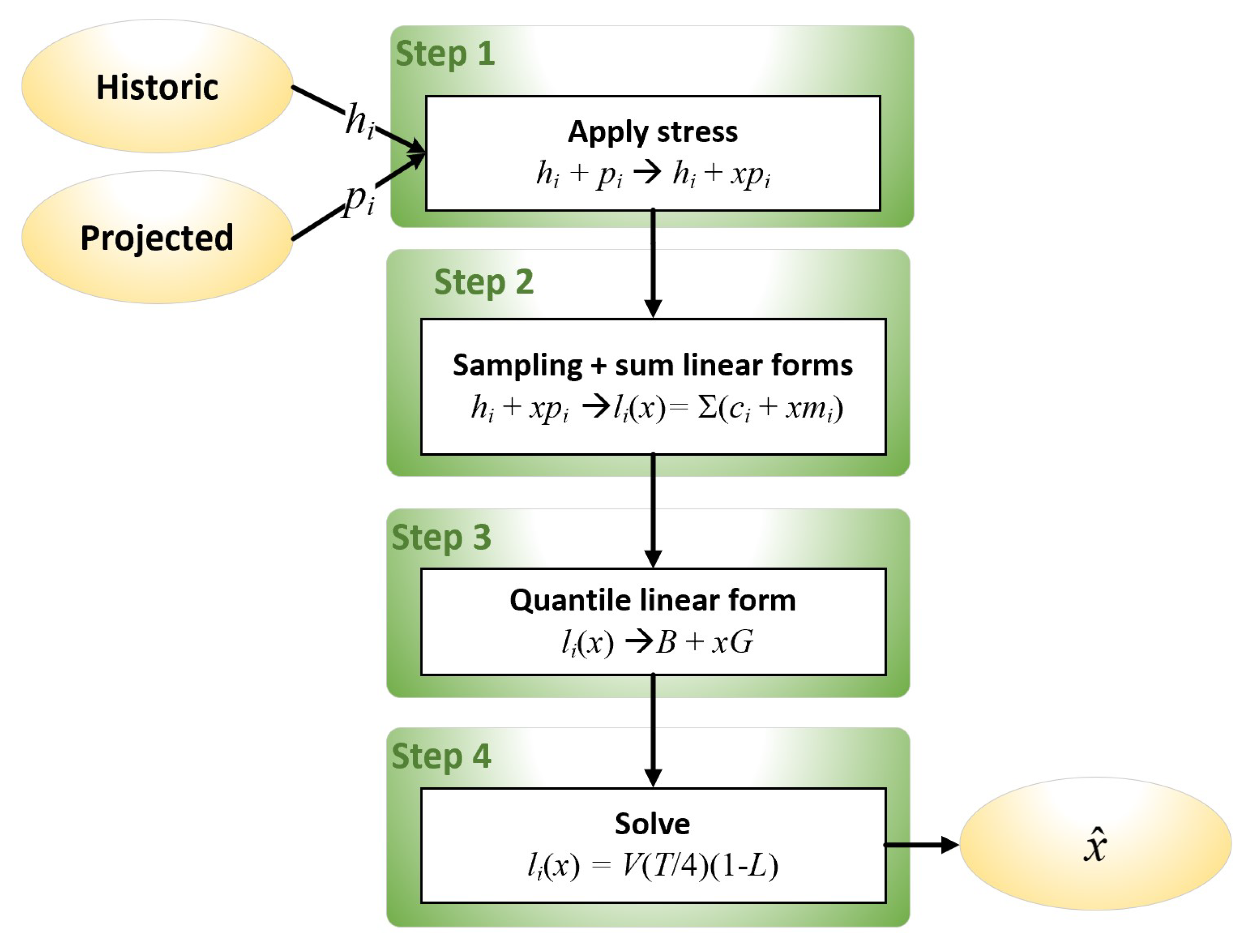
Consider a set of H historic operational risk losses h 1 , h 2 , . . . , h H and a (smaller) set of P projected losses p 1 , p 2 , . . . , p P (for example, for the next quarter). When stressed with the stress factor x, random samples can be drawn from the set { l 1 , l 2 , . . . , l H , x p 1 , x p 2 , . . . , x p P } (Step 2b in Appendix A). Each set of random samples is summed (Step 2c in Appendix A). In each case, the sum is expressed as a linear function of x. Step 3 in Appendix A is to extract the 99.9 percentile of those sums. In numerical work, that task is easy: the elements in a vector of sums are ordered, and the correct element is extracted. Ordering linear expressions of the form c i + x m i ( c i , m i I R ) is non-trivial, and we adopt an approximation, using the values of the c i and m i and based on the marginal effect of stressing projected data.
The major steps are shown in Figure 2. They are elaborated upon in the symbolic linear algorithm. The stage marked (**) corresponds to the stages marked in the same way in the LDA algorithm in Appendix A.
Symbolic Linear Algorithm
  • Apply stress
    (a)
    Stress projected losses p i x p i
    (b)
    Calculate distributions and parameters for historic and projected losses
  • Derive linear forms
    (a)
    Sample linear forms { c i + x m i } from the set { h i + x p i }
    (b)
    Sum linear forms: Σ ( c i + x m i )
  • Derive a quantile linear form
    (a)
    Calculate the 99.9 quantiles, Q 0 and Q 1 , of the linear forms c i + x m i when x = 0 and x = 1 . The difference Q 1 Q 0 measures the effect of including unstressed data. This stage establishes a base value for calculating stress.
    (b)
    Calculate the gradients, g i , of each linear form c i + x m i , and extract the 99.9 quantile, G, from the set of g i (**)
    (c)
    Assert that the line Q 1 Q 0 + x G should be the required quantile linear form. This line measures the linear deviation from the base value as x increases.
  • Solve for x
    (a)
    Solve the (linear) equation Q 1 Q 0 + x G = V ( T 4 ) ( 1 L ) for a 1 quarter prediction. V and L are the same as in Equation (2), and T is an annual inflation factor for VaR, such as 0.5 for 50% annual inflation. For projection 1 year ahead, V T ( 1 L ) would be used instead. The solution, x , represents a marginal stress factor, representing the amount of the inflated VaR.
    (b)
    The overall stress factor, referred to the original capital, V, is returned as x ^ = 1 + x .
The Mathematica code in Appendix B shows the procedure that implements the above algorithm. The algorithm should be seen both as a heuristic and a practical proposition. It has the advantage that only one long LDA evaluation is needed. Other methods considered in this paper need at least three in most cases. The results produced tend to be over-estimates (by about 8%; see Section 6.7). Memory requirements are more stringent than for numeric calculations, as a large number of symbolic expressions must be held in RAM prior to extracting one of them to represent a quantile expression. A symbolic approach does, however, allow the possibility of applying non-linear stress to the projected losses.

6. Results

6.1. Data and Implementation

The OpRisk loss data set used was extracted from a dedicated OpRisk database and spanned the period from January 2010 to December 2019. Basel risk class Clients, Products and Business Practice was excluded because of distortions introduced by extreme losses and in accordance with BoE directives. We refer to this data set as nonCPBP.
Referring to the five-year data window described in Section 4.1, the data in each five year window were a good fit to a log normal distribution at a 95% confidence level. The log normal μ parameters ranged from 9.723 to 10.538, with a mean of 9.971. The log normal σ parameters ranged from 1.999 to 2.291 with a mean of 2.147. These values are typical for OpRisk data. The mean VaR of the last five windows, which represents the most recent data, was 213.2. The mean of the entire data set was approximately 364,000, whereas the maximum three values were 61.35 million, 49.02 million and 32.82 million. The small mean, coupled with very large maximum values, are typical of fat-tailed data (Fat-tailed data are characterised by a distribution whose tail decays according to a power law).
All calculations were done using the R statistical programming language (https://www.r-project.org/, accessed on 28 April 2021), with particular emphasis on the lubridate and dplyr packages for date manipulation and data selection, respectively. Mathematica Version 12 was used for graphics, dynamic illustrations and the approximate optimization method that makes use of symbolic computation (Section 5).

6.2. Previous Results

The OpRisk-VaR context has not been considered before by other authors. We have published extensive results for zero acquisition, including comparisons with “established” acquisition functions. They may be found in [35,36]. Those results are too extensive to reproduce in full in this paper, but we do report a summary of them below. In this paper, we supplemented zero acquisition with a range of alternative optimizations. Thus, we can contrast the main results for “established” acquisition functions with the alternatives. One further comparison is possible. We noted that some other authors have used very few Monte Carlo trials in their analyses ([25,29], for example). Although their contexts were very different from ours, we can find what happens if we use a low number of Monte Carlo trials. The results are in Section 6.5.
For later reference, we refer to the “established” acquisition functions (EI, POI and CB) as Block 1 methods and the “zero” acquisition functions (ZLCB and ZUCB) as Block 2. Other acquisition functions (SE and KG-GP) are referred to as Block 3 methods. Methods that do not use acquisition functions (KG, BS, LI and RS) are referred to as Block 4 methods.
The main findings from [35,36] were (the list below shows the means of run numbers with standard deviations in square brackets):
  • For one million Monte Carlo trials using Block 1 (“traditional”) methods: 15.64 [11.90]
  • For three million Monte Carlo trials using Block 1 (“traditional”) methods: 12.49 [9.24]
  • For five million Monte Carlo trials using Block 1 (“traditional”) methods: 13.35 [10.25]
  • For one million Monte Carlo trials using Block 4 (“random”) methods: 12.42 [12.56]
  • For three million Monte Carlo trials using Block 4 (“random”) methods: 16.12 [12.01]
  • For five million Monte Carlo trials using Block 4 (“random”) methods: 10.84 [10.88]
  • For one million Monte Carlo trials using Block 2 (zero) methods: 7.25 [5.42]
  • For three million Monte Carlo trials using Block 2 (zero) methods: 5.43 [3.52]
  • For five million Monte Carlo trials using Block 2 (zero) methods: 5.44 [3.41]
A qualitative summary of previous results is that Block 1 (“traditional”) methods have the same performance characteristics as random selection, and that zero acquisitions approximately halves both the “traditional” means and standard deviations run number. In the sections that follow, our current results are compared to our previous results.

6.3. Run Number Expected Value Results

The run number expected values presented in Table 2 follow the order (Blocks 1 to 4) in which they were introduced in Section 2.1.
The most notable observation from Table 2 is the poor performance of all methods in Block 1 compared to their corresponding Block 2 methods (the zero acquisitions). The Block 1 method expected values were similar to the random selection (RS) method in Block 4. The degree of improvement introduced by the zero methods was considerable. The Block 3 methods provided some improvement on LCB and UCB, but not as much as the zero methods. In contrast, the Block 4 methods excluding RS were comparable to the zero methods.
Table 2 reveals two broad trends. First, accuracy (i.e., a minimal run number) generally improved with an increasing number of Monte Carlo iterations. Second, for CB methods, accuracy was usually better for a lower value of κ . This indicated that exploration (i.e., searching away from the GP-suggested mean) was an inferior policy.

6.4. Standard Deviation Results

The run number standard deviations are shown in Table 3.
The standard deviation results were similar. Zero acquisition (Block 2) outperformed the Block 1 methods by a considerable margin. The zero methods were notable because their standard deviations were less than their corresponding expected values. For Block 1 methods, the standard deviations were approximately the same size as their corresponding expected values. The real gain, when the standard deviation was less than two, was that long runs in which the sequence of “expensive” fits failed to attain the required target were almost eliminated. The BS method was particularly good in this respect.

6.5. Results from a Few Monte Carlo Trials

Studies in other contexts have used very few Monte Carlo trials in their analyses ([25]: 10,000 trials; [29]: 1000, for example). There are no direct comparisons of our work with the work of other authors. As a crude comparison, Table 4 shows the results of running the binary and zero (with κ = ± 0.75 ) methods with only 10,000 Monte Carlo trials. In practice, we would only do that to ensure that the software works correctly. The random selection method is included as a comparison.
Table 4 shows that the benefits of zero and binary acquisition were lost with only 10,000 Monte Carlo trials. Both run number means and standard deviations were unacceptably high. We concluded that other contexts are more stable with respect to the optimization processes used, although precise characteristics were not apparent in the papers concerned. The OpRisk-VaR is essentially different because of the stochastic nature of calculating VaR with fat-tailed data. We observed that extreme VaR values can be obtained if outliers are generated in random sampling.

6.6. Run Number 95% Confidence Interval

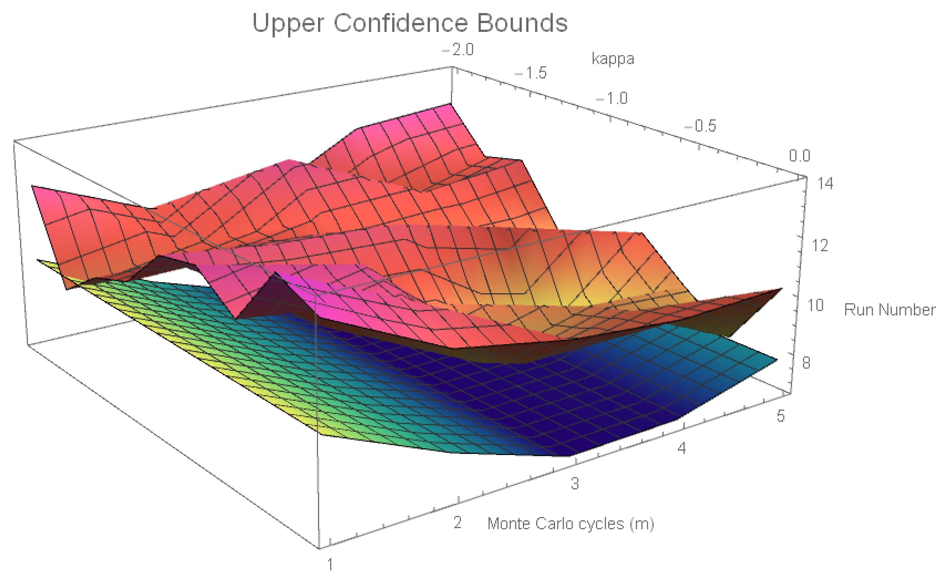
Figure 3 shows a comparison of two of the optimal optimization methods that proved to be viable methods for solving the optimisation problem in Equations (2) and (3). ZLCB and ULCB were approximately equivalent in terms of expected run number. However, BS beat them on the standard deviation. The figure shows ZLCB and BS. The 3D plots illustrate surfaces for the upper limit of 95% (two-tailed) confidence intervals for the variation of run number with the number of Monte Carlo iterations and κ . With the notation in Equation (17) and assuming normally distributed R , the upper limit of this interval is given by R ¯ + 1.96 ( v a r ( R ) .

6.7. Optimal Value Consistency Results

The consistency of the calculated optimal values returned by the optimisation (i.e., x ^ in Equations (2) and (3)) was examined by running the same set of trials repeatedly. The means of 1–5 m Monte Carlo cycles for viable (in terms of expected run number) optimisation methods only were considered. Table 5 shows that BS was the preferable method, since the BS SD was approximately half the size of the others, although all were of acceptable consistency.
Five hundred independent trials of the approximate analytical method (Section 5) gave a mean value for x ^ of 1.1779, with a standard deviation of 0.0285. That represents an overestimate relative to those in Table 5 of approximately 7.3%.

6.8. Timings

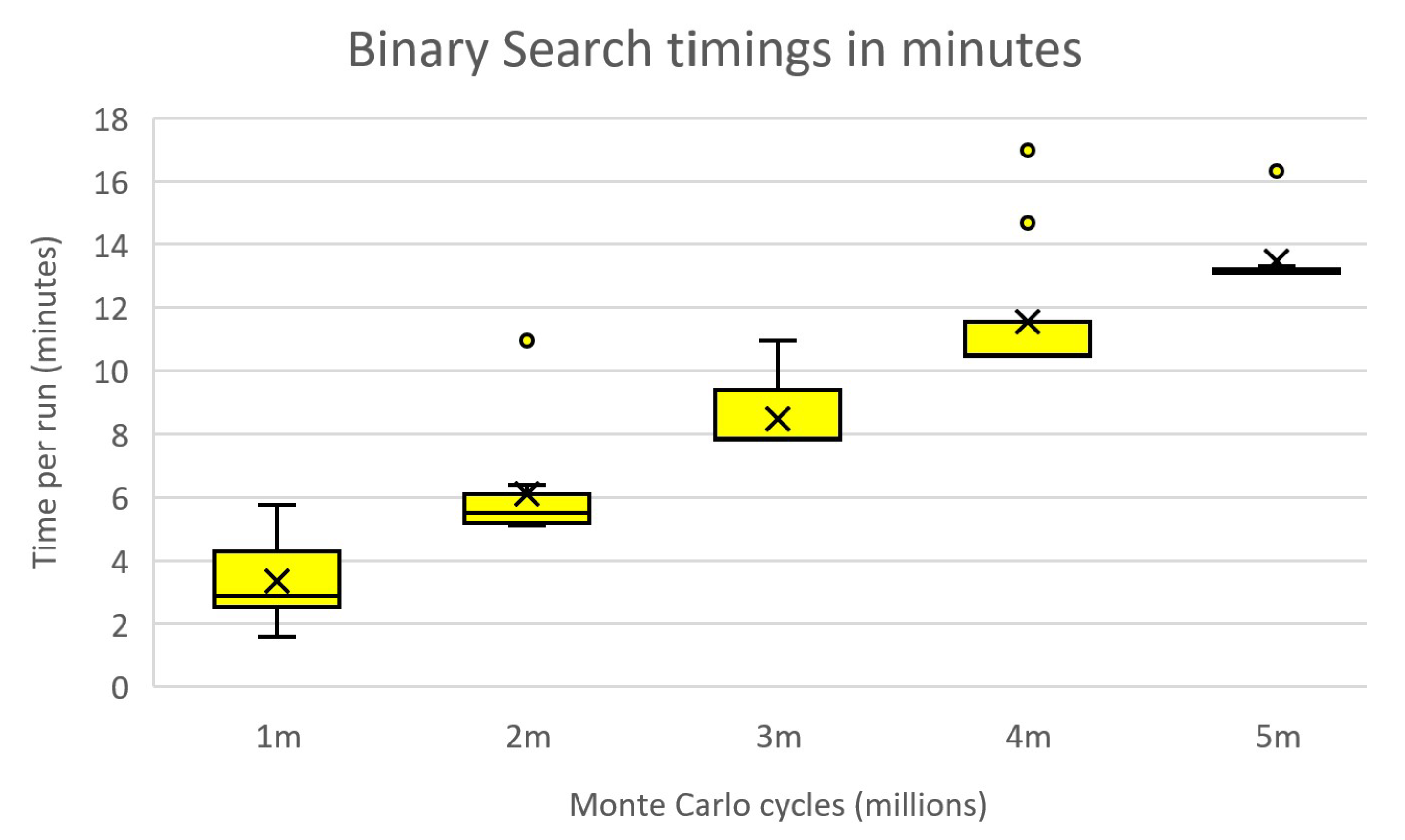
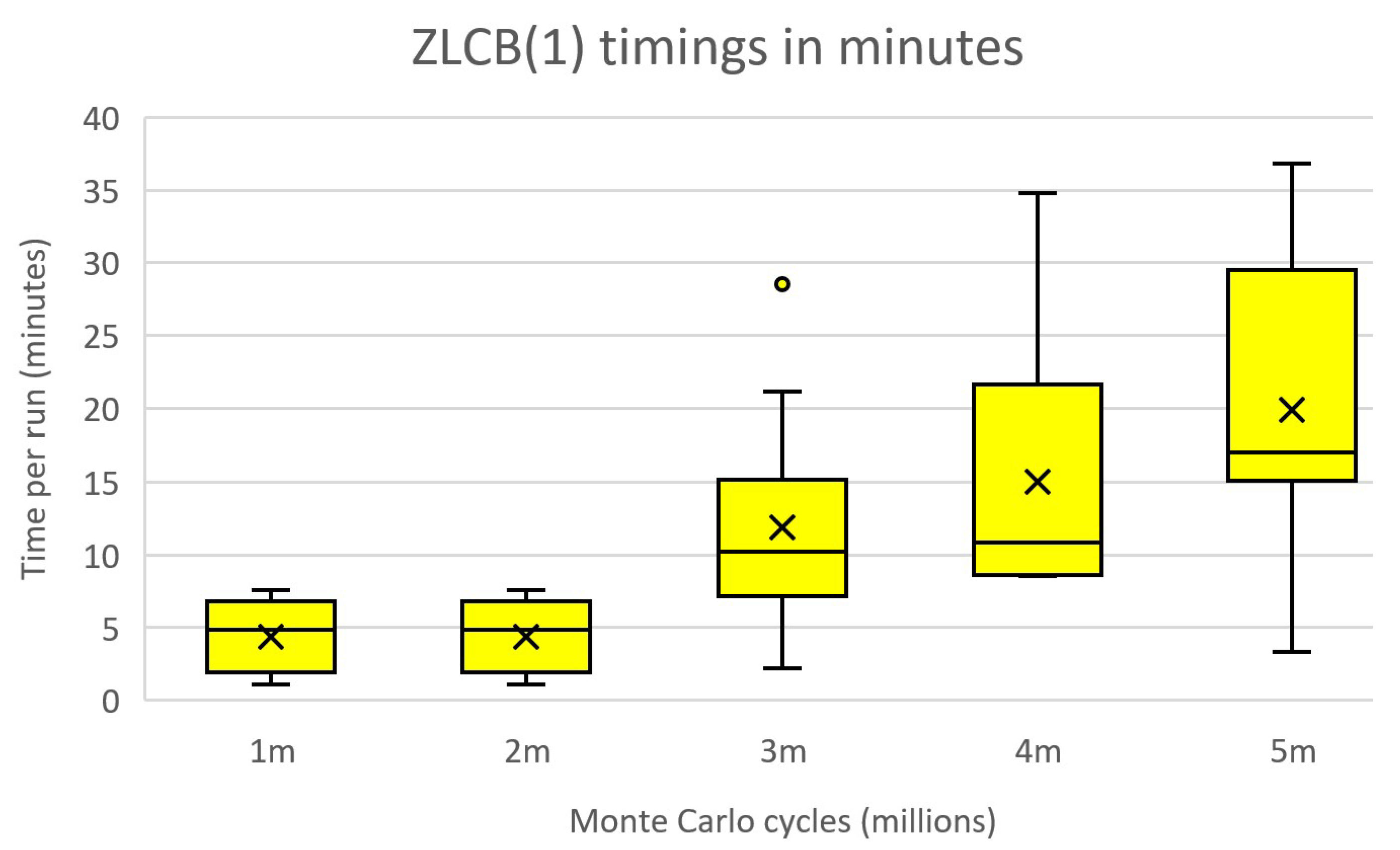
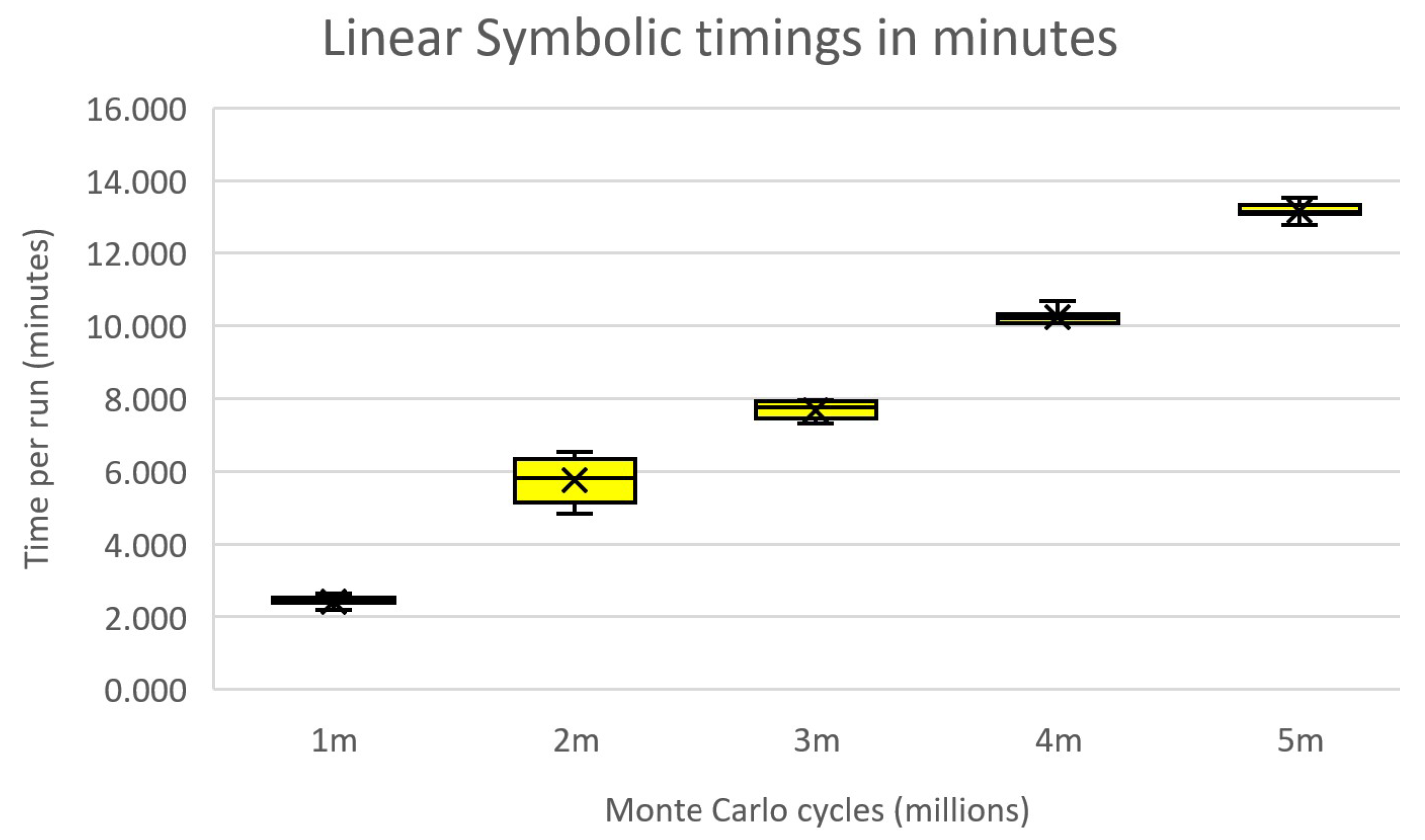
Figure 4 and Figure 5 summarise the times taken to complete each run using binary search and ZLCB acquisition, respectively, using the number of Monte Carlo cycles indicated. There was a near linear progression of the mean run time with increasing number of Monte Carlo cycles, as might be expected, in both cases. For the binary case, the SDs showed no discernible trend, although the spread was remarkably small in the 5 m case. The major improvement was as far as three million Monte Carlo iterations. Beyond that point, outliers persisted, and the time taken to complete a large number of independent runs became excessive. The spreads were much more apparent in the ZLCB case, but appeared to increase as the number of Monte Carlo iterations increased. Therefore, using more than three million was not necessary.
Figure 6 shows box plots for the timings of symbolic optimization using the approximate analytical method described in Section 5. The most apparent difference between it and Figure 4 and Figure 5 is the extremely small box heights with a lack of outliers. Per single Monte Carlo run (note that the approximate analytical method needs only one, whereas others need at least three), the approximate analytical route was slower: Mathematica was usually slower than R.

6.9. The Effect of COVID-19

The COVID-19 pandemic has resulted in extreme economic stress, some of which is reflected in operational risk losses, even though they are non-financial. Consequently, it is useful to see what economic stress should be applied to operational risk losses in case there is a need to increase capital (i.e., VaR) significantly. The symbolic computation method of Section 5 provides a quick and easy way to estimate the required stress factors. There are indications from Risk.net (see https://www.risk.net/comment/7652866/op-risk-data-losses-plummet-during-lockdown, accessed on 28 April 2021) that some banks’ operational risk losses have fallen significantly due to much reduced activity. Therefore, we calculated what stress factor would be needed if activity, as measured by the number of predicted transactions, falls by up to 50%. Figure 7 shows the results of trials of random reductions of predicted transactions centred on 25% and 50% (with a sample size of 500 for each). Note that they are likely to all be slight overestimates. As a direct comparison, the “zero” predicted transaction reduction mean was 1.176, and the SD was 0.112. Each set took about 40 min to complete. The mean results were as expected: as activity reduced, the required stress to maintain the same capital increased.

7. Discussion

Table 2 gives an indication of what value of κ to use to give optimal results. We suggested κ ( 0.5 , 0.75 ) . The stochastic nature of the LDA-based evaluation of g makes it unsafe to pick an actual minimum based on any particular value of κ . It is more straightforward to select an appropriate number of Monte Carlo cycles to use. The more there are, the better, but using more takes longer.
We also noted informally that for BS, LI, KG and zero optimisations, there was a steady reduction in the error function g ( x ) as the run number increased, until the condition g ( x ) < L was met. That did not occur with the other methods considered. In those cases, the sequence of error function values looked more like the results of a random parameter value selection.

7.1. Implications for Practitioners

For users (developers and risk analysts), the implications of this study are clear. First, the proposed methods for RST are appropriate and work successfully in the context of OpRisk, as shown by the results in Section 6.3 and Section 6.4. For risk analysts, the issue is to balance the accuracy of testing with the time taken to achieve that accuracy. Although in the following section, we recommend the binary search method, others might accept the zero method because the expected run number is lower. For the zero method, we suggest using 10 distinct runs, each of three million Monte Carlo trials. For the binary search method, we recommend 10 distinct runs, each of one million Monte Carlo trials. Generally, there is little to be gained by using more than three million. If time is an issue, in both cases, we would agree to 10 runs, each with Monte Carlo trials of 500,000, and would take care to add note wider error bounds. We encourage developers to calculate 95% error bounds as a matter of course.
Hitherto, regulators have not paid attention to RST. The COVID-19 pandemic has prompted the U.K. regulator to use RST for its dedicated COVID economic scenario, and they may do so to model severe economic conditions in the future. We speculate that regulators have not understood how to implement RST processes, and we hope to inform them in this paper. RST models in other contexts (see Section 3.2) show that since 2018, there has been increased interest in research on RST, with an emphasis on modelling systemic risk. This is of vital importance to society, since the banking system underpins other commercial activity. The implication of informative stress testing (reverse or not) has a profound implication for banks. If too much capital is retained, the banking business model is not sustainable because banks cannot lend.
As a general direction for research, we consider that seeking simple solutions for simple problems will be fruitful. We demonstrated that “established” BO acquisition functions (EI, POI and CI) do not work well in the “simple” context of OpRisk-VaR. The “simple” solution is to square the acquisition function (Equation (5): μ n 1 ( x i ) κ σ n 1 ( x i ) ( μ n 1 ( x i ) κ σ n 1 ( x i ) ) 2 ). We speculate that the same solution may work in other contexts.

7.2. Contribution to the Literature

We summarise the contribution to the corpus of knowledge, with particular reference to the OpRisk community, as follows.
  • This work is the first application of RST in the context of OpRisk. It is both simple conceptually and easy to apply in practice.
  • The U.K. regulatory authority has hitherto avoided discussion of how stress testing (reverse or not) should be done. We provided a first solution.
  • The use of “traditional” acquisition functions in Bayesian optimization has been shown to be ineffective in the context of OpRisk. A simple solution, the ZERO acquisition function, was defined and found to be performant.
  • Two performant optimization methods, zero and binary, were identified as optimally performant in the context of OpRisk.

8. Conclusions

The justification for using zero acquisition in place of any of the Block 1 methods is ultimately empirical. The improvement in the mean and standard deviation run number is compelling, even in the absence of any theoretical justification.
The results in Section 6.8 show that the number of Monte Carlo cycles used depends mostly on the time available. A large number, as well as a small number, can generate outliers. It is therefore more important to carry out as many independent runs as possible: ideally between two and three million.
Overall, in practice, binary search is the “least risk” optimisation procedure. It gives a combination of low values for the run number mean and standard deviation, with a low standard deviation for the optimal parameter value. The linear interpolation and knowledge gradient methods produce marginally worse results on all of those metrics. Although optimisation using zero acquisition has a lower run number expected value than binary search, the corresponding standard deviation is higher, and optimal parameter accuracy is also impaired slightly. The final decision therefore depends on what property is valued most. If it is speed, then zero acquisition is preferable. If it is consistency, then binary search is preferable. We favour the second of these options.

Further Work

The results of the symbolic approach in Section 5 are encouraging and open the possibility of a more general approach. Using a generic function, G, in place of the specific linear transformation of projected losses would allow the application of non-linear transformations by supplying G as a function argument. For example, G ( x ) = x { P } , where x is a stress factor to be determined and { P } is a set of predicted losses, would model preferential inflation of large losses.

Funding

This research received no external funding.

Conflicts of Interest

The author declares no conflict of interest.

Appendix A. The LDA Algorithm

This Appendix shows the essential stages in the LDA algorithm of Frachot et al. [3]. The stages marked (**) were referred to in Section 5. Given N losses over y years, with m Monte Carlo iterations and a fitted severity distribution F:
  • Calculate the annual loss frequency, f = N y
  • Repeat m times
    (a)
    Obtain a frequency sample size λ by drawing a random sample of size 1 from a Poisson (f) distribution (*) (**)
    (b)
    Draw a sample of size λ , S λ , from the severity distribution, F (**)
    (c)
    Sum the losses in S λ to obtain Σ S λ , the annual loss estimate, and add to a vector of annual loss estimates (**)
  • Calculate VaR: the 99.9 th percentile of the vector of annual loss estimates.
(*) A Poisson distribution is not the only way to do this. A negative binomial distribution is often used.
For the R and Mathematica implementations, the inputs are:
  • data: a vector of numbers n1, n2, ....
  • params: the log normal parameters fitted to data
  • years: the number of years covered by the data
  • m: the number of Monte Carlo iterations
  • threshold: the minimum datum for modelling purposes.
In both cases, the output is the 99.9% value-at-risk.
LDA Implementation in R
# Call:
# data <- c(n1, n2, ....); LDA(data, c(10,2), 5, 1000000, 10)
LDA <- function(data, params, years, m, threshold)
{
 data <- data[data>threshold]
 freq <- length(data)/years
 xSum <- numeric(m)
 for (t in 1:m)
 {
     # Apply a frequency correction: freq1 = freq/Prob(loss>threshold)
     cdf <- plnorm(threshold, params[1], params[2])
     freq1 <- freq/(1 - cdf)
     n <- rpois(1, freq1)
     x <- rlnorm(n, params[1], params[2])
     xSum[t] <- sum(x)
 }
 xSum <- sort(xSum)
 var <- xSum[ceiling(0.999*length(xSum))]
 return(var)
}
LDA Implementation in Mathematica
(* Call:
 data = {n1, n2, ....}
 LDA1[data, {10, 2}, 5, 1000000, 10] *)
LDA[data_, params_, years_, m_, threshold_] :=
 Module[{data1, freq, mu, sigma, var, xSum, p, n},
     data1 = Select[data, (# > threshold)&];
     freq = Ceiling[Length[data1]/years];
     p = Length[data1]/Length[data];
     freq = Ceiling[freq/p]; (* Frequency correction for threshold *)
     mu = First[params]; sigma = Last[params];
     xSum = Map[(n = RandomVariate[PoissonDistribution[freq], 1];
     RandomVariate[LogNormalDistribution[mu, sigma, n] /.
         List -> Plus) &, Array[# &, m]];
     xSum = Sort[xSum];
     var = xSum[[Ceiling[0.999*Length[xSum]]]]
 ]

Appendix B. Mathematica Code Implementing Algorithm Symbolic Linear

The Mathematica code in this Appendix is an implementation of the symbolic linear algorithm in Section 5.
(* Inputs:
lin: the set of linear forms from sampling
q: 0.999, the 99.9 quantile
x: the output variable *)
(* Call:*)
eq = LinearQuantile[lin, q, x]
xprime = Solve[eq == V (T/400) (1 - L), x]; xhat = 1 + First[x /. xprime]
LinearQuantile[lin_, q_, x_] :=
 Module[{lin1, lin0, q1, q0, EQ, m, c, mc, mc2, G, B},
     (* Calculate the ``base’’ quantile *)
     lin1 = lin /. x -> 1; lin0 = lin /. x -> 0;
     q1 = FindQuantile[lin1, q][[1, 1]]; q0 = FindQuantile[lin0, q][[1, 1]];
     B = lin1[[q1]] - lin0[[q0]];
     (* Calculate the ``gradient’’ quantile *)
     mc = Map[ (lin[[#]] /. {c__ + x m__} -> {c, m}) &,
     Array[# &, Length[lin]] ];
     mc2 = Map[Last, mc];
     G = FindQuantile[mc2, q][[1, 1]];
     EQ = B + x mc2[[G]]
]
FindQuantile[arr_, q_] :=
 Module[{arrS, tgt, pos},
     arrS = Sort[arr];
     tgt = arrS[[Ceiling[q Length[arr]]]];
     pos = Position[arr, tgt]
]

References

  1. Mitic, P. A Framework for Analysis and Prediction of Operational Risk Stress. Math. Comput. Appl. 2021, 26, 19. [Google Scholar]
  2. Basel Committee on Banking Supervision. International Convergence of Capital Measurement and Capital Standards, Clause 644. 2006. Available online: https://www.bis.org/publ/bcbs128.pdf (accessed on 8 February 2021).
  3. Frachot, A.; Georges, P.; Roncalli, T. Loss Distribution Approach for Operational Risk; Working paper; Groupe de Recherche Operationnelle, Credit Lyonnais: Paris, France, 2001; Available online: http://ssrn.com/abstract=1032523 (accessed on 16 December 2020).
  4. Basel Committee on Banking Supervision. BCBS196: Supervisory Guidelines for the Advanced Measurement Approaches. 2011. Available online: https://www.bis.org/publ/bcbs196.pdf (accessed on 17 March 2021).
  5. Grundke, P. Reverse stress tests with bottom-up approaches. J. Risk Model Valid. 2011, 5, 71–90. [Google Scholar] [CrossRef] [Green Version]
  6. Bank of England. Stress Testing the UK Banking System: Key Elements of the 2021 Stress Test. 2021. Available online: https://www.bankofengland.co.uk/stress-testing/2021/key-elements-of-the-2021-stress-test (accessed on 12 March 2021).
  7. Mockus, J. On Bayesian methods for seeking the extremum, In Optimization Techniques IFIP Technical Conference; Springer: Berlin/Heidelberg, Germany, 1974; pp. 400–404. Available online: http://dl.acm.org/citation.cfm?id=646296.687872 (accessed on 9 March 2021).
  8. Cox, D.D.; John, S. A statistical method for global optimization. In Proceedings of the 1992 IEEE International Conference on Systems, Man, and Cybernetics, Chicago, IL, USA, 18–21 October 1992. [Google Scholar]
  9. Kushner, H.J. Stochastic model of an unknown function. J. Math. Anal. Appl. 1962, 5, 150–167. [Google Scholar] [CrossRef] [Green Version]
  10. Mockus, J.; Tiesis, V.; Zilinskas, A. The application of Bayesian methods for seeking the extremum. Towards Glob. Optim. 1978, 2, 2. [Google Scholar]
  11. Picheny, V.; Wagner, T.; Ginsbourger, D. A Benchmark of Kriging-Based Infill Criteria for Noisy Optimization. Struct. Multidiscip. Optim. 2013, 48, 607–626. [Google Scholar] [CrossRef] [Green Version]
  12. Rasmussen, C.E.; Williams, C.K.I. Gaussian Processes for Machine Learning; MIT Press: Boston, MA, USA, 2006. [Google Scholar]
  13. Murphy, K.P. Machine Learning: A Probabilistic Perspective, Chapter 15; MIT Press: Boston, MA, USA, 2012. [Google Scholar]
  14. Gardner, J.R.; Kusner, M.J.; Xu, Z.; Weinberger, K.Q.; Cunningham, J.P. Bayesian Optimization with Inequality Constraints. In Proceedings of the 31st International Conference on International Conference on Machine Learning (ICML’14), Beijing, China, 22–24 June 2014; Volume 32, pp. II-937–II-945. Available online: https://dl.acm.org/doi/10.5555/3044805.3044997 (accessed on 18 March 2021).
  15. Gramacy, R.B.; Gray, G.A.; Le Digabel, S.; Lee, H.K.H.; Ranjan, P.; Wells, G. Modeling an Augmented Lagrangian for Blackbox Constrained Optimization. Technometrics 2016, 58, 1–11. [Google Scholar] [CrossRef]
  16. Wang, H.; Stein, B.; Emmerich, M.; Back, T. A new acquisition function for Bayesian optimization based on the moment-generating function. In Proceedings of the 2017 IEEE International Conference on Systems, Man, and Cybernetics (SMC), Banff, AB, Canada, 5–8 October 2017; pp. 507–512. [Google Scholar]
  17. de Freitas, N.; Smola, A.; Zoghi, M. Exponential regret bounds for Gaussian Process bandits with deterministic observations. In Proceedings of the 29th International Conference on International Conference on Machine Learning (ICML’12), Edinburgh, Scotland, UK, 26 June–1 July 2012; pp. 955–962. Available online: https://dl.acm.org/doi/10.5555/3042573.3042697 (accessed on 18 March 2021).
  18. Merrill, E.; Fern, A.; Fern, X.; Dolatnia, N. An Empirical Study of Bayesian Optimization: Acquisition Versus Partition. J. Mach. Learn. Res. 2021, 22, 1–25. Available online: https://www.jmlr.org/papers/volume22/18-220/18-220.pdf (accessed on 18 March 2021).
  19. Hennig, P.; Schuler, C.J. Entropy search for information-efficient global optimization. J. Mach. Learn. Res. 2012, 13, 1809–1837. [Google Scholar]
  20. Frazier, P.I.; Powell, W.B.; Dayanik, S. The Knowledge-Gradient Policy for Correlated Normal Beliefs. Informs J. Comput. 2009, 21, 599–613. [Google Scholar] [CrossRef] [Green Version]
  21. Williams, L.F. A modification to the half-interval search (binary search) method. In Proceedings of the 14th Annual Southeast Regional Conference (ACM-SE 14), Birmingham, AL, USA, 22–24 April 1976; pp. 95–101. Available online: https://doi.org/10.1145/503561.503582 (accessed on 8 February 2021).
  22. Powell, W.B.; Ryzhov, I.O. Optimal Learning Chapter 5; Wiley: Hoboken, NJ, USA, 2012. [Google Scholar]
  23. Letham, B.; Karrer, B.; Ottoni, G.; Bakshy, E. Constrained Bayesian Optimization with Noisy Experiments. Bayesian Anal. 2019, 14, 495–519. Available online: https://projecteuclid.org/journals/bayesian-analysis/volume-14/issue-2/Constrained-Bayesian-Optimization-with-Noisy-Experiments/10.1214/18-BA1110.full (accessed on 14 March 2021). [CrossRef]
  24. Baes, M.; Schaanning, E. Reverse Stress Testing: Scenario Design for Macroprudential Stress Tests. Available online: http://dx.doi.org/10.2139/ssrn.3670916 (accessed on 12 April 2021).
  25. Montesi, G.; Papiro, G.; Fazzini, M.; Ronga, A. Stochastic Optimization System for Bank Reverse Stress Testing. J. Risk Financ. Manag. 2020, 13, 174. [Google Scholar] [CrossRef]
  26. Grigat, D.; Caccioli, F. Reverse stress testing interbank networks. Sci. Rep. 2017, 7, 15616. [Google Scholar] [CrossRef] [Green Version]
  27. Eichhorn, M.; Mangold, P. Reverse Stress Testing for Banks: A Process-Orientated Generic Framework. J. Int. Bank. Law Regul. 2016, 4. Available online: https://www.cefpro.com/wp-content/uploads/2019/07/Eichhorn_Mangold_2016_JIBLR_Issue_4_Proof_3.pdf (accessed on 13 April 2021).
  28. Albanese, C.; Crepey, S.; Stefano, I. Reverse Stress Testing. 2020. Available online: http://dx.doi.org/10.2139/ssrn.3544866 (accessed on 12 April 2021).
  29. Grundke, P.; Pliszka, K. A macroeconomic reverse stress test. Rev. Quant. Financ. Account. 2018, 50, 1093–1130. [Google Scholar] [CrossRef] [Green Version]
  30. Bank of England. Stress Testing. Available online: https://www.bankofengland.co.uk/stress-testing (accessed on 16 December 2020).
  31. Financial Conduct Authority. FCA Handbook April SYSC 2021; Chapter 20. Available online: https://www.handbook.fca.org.uk/handbook/SYSC/20/ (accessed on 13 April 2021).
  32. European Central Bank. 2020 EU-Wide Stress Test—Methodological Note. Available online: https://www.eba.europa.eu/sites/default/documents/files/document_library/2020%20EU-wide%20stress%20test%20-%20Methodological%20Note_0.pdf (accessed on 16 December 2020).
  33. European Systemic Risk Board. Macro-Financial Scenario for the 2021 EU-Wide Banking Sector Stress Test. 2021. Available online: https://www.esrb.europa.eu/mppa/stress/shared/pdf/esrb.stress_test210120 0879635930.en.pdf ?a0c454e009cf7fe306d52d4f35714b9f (accessed on 13 April 2021).
  34. US Federal Reserve Bank. Stress Tests and Capital Planning: Comprehensive Capital Analysis and Review. 2020. Available online: https://www.federalreserve.gov/supervisionreg/ccar.htm (accessed on 18 December 2020).
  35. Mitic, P. Bayesian Optimization for Reverse Stress Testing. In Advances in Intelligent Systems and Computing; Vasant, P., Zelinka, I., Gerhard-Weber, G.M., Eds.; Springer: Cham, Switzerland, 2021; Chapter 17. [Google Scholar] [CrossRef]
  36. Mitic, P. Improved Gaussian Process Acquisition for Targeted Bayesian Optimization. Int. J. Model. Optim. 2021, 11, 12–18. [Google Scholar] [CrossRef]
  37. Wilson, J.T.; Hutter, F.; Deisenroth, M.P. Maximizing acquisition functions for Bayesian optimization. In Proceedings of the 32nd International Conference on Neural Information Processing Systems (NIPS’18), Montréal, QC, Canada, 3–8 December 2018; Available online: https://dl.acm.org/doi/10.5555/3327546.3327655 (accessed on 13 April 2021).
  38. Srinivas, N.; Krause, A.; Kakade, S.; Seeger, M. Gaussian Process Optimization in the Bandit Setting: No Regret and Experimental Design. In Proceedings of the 27th International Conference on International Conference on Machine Learning (ICML’10), Haifa, Israel, 21–24 June 2010; pp. 1015–1022. Available online: http://dl.acm.org/citation.cfm?id=3104322.3104451 (accessed on 8 February 2021).
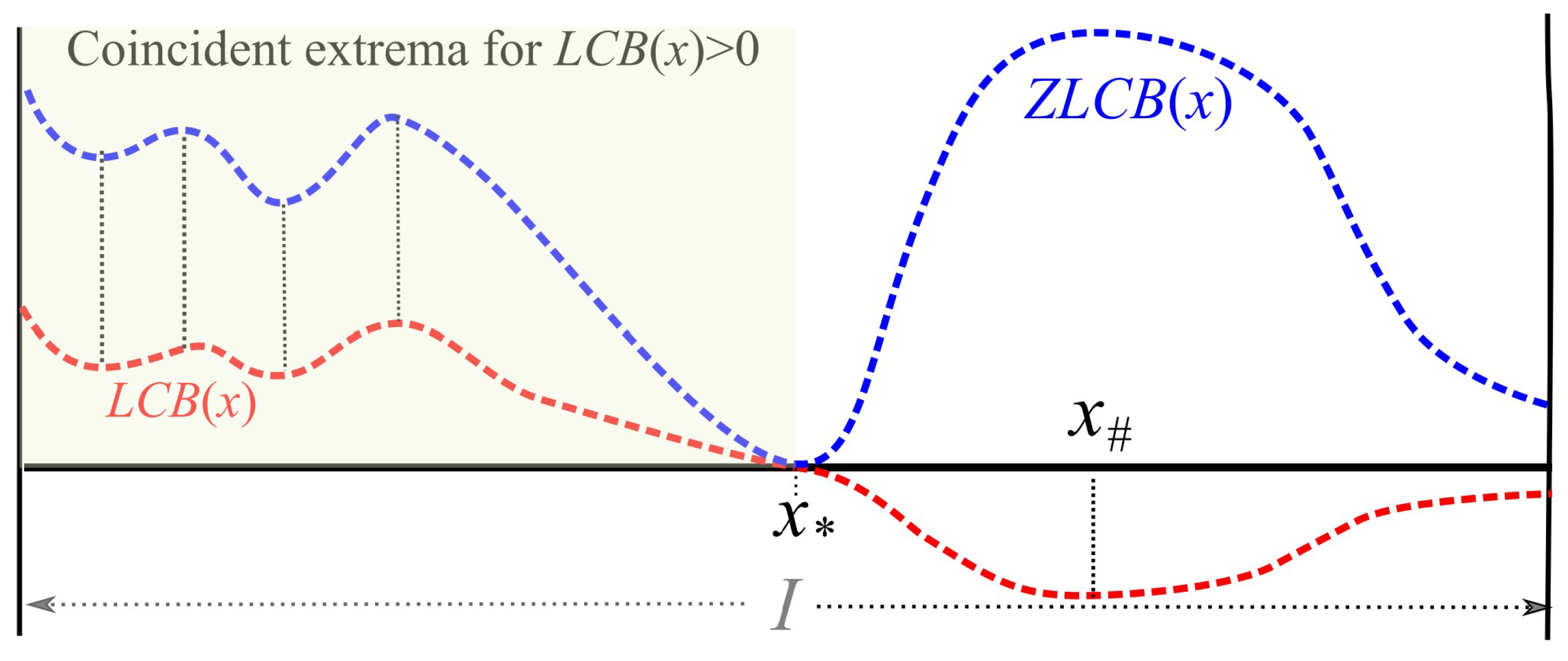
Figure 1. E ( n 1 , x ) in the interval I for ZLCB and LCB, showing minimum value next proposals x * and x , respectively.
Mca 26 00038 g001
Figure 2. Major steps in the symbolic linear algorithm.
Mca 26 00038 g002
Figure 3. Upper confidence bounds: ZLCB (red-purple) and BS (blue-green)
Mca 26 00038 g003
Figure 4. Box plot timings for binary search optimisation: 10 runs in each case.
Mca 26 00038 g004
Figure 5. Box plot timings for ZLCB κ = 1 optimisation: 10 runs in each case.
Mca 26 00038 g005
Figure 6. Box plot timings for linear symbolic optimisation: 10 runs in each case.
Mca 26 00038 g006
Figure 7. COVID-19 reduced activity scenarios, each with 25,000 Monte Carlo iterations. The vertical dashed lines show the position of the means.
Mca 26 00038 g007
Table 1. Optimization framework: principal steps.
StepOperationComment
1 V = f ( D , x = 1 ) Historic VaR, no inflation
2 V ^ = V ( 1 + p 100 ) Inflated VaR by p%
3 V ^ = f ( D ( 1 + x ) ) Formulate expression for the VaR of scaled data
4 | V ^ V V |   < L Formulate expression for the relative change in VaR
5 x ^ = a r g m i n x I ( | V ^ V V | < L ) Solve for x (Equation (2))
Table 2. Run number expected values, based on 25 runs in each case. * When κ = 0 the upper and lower CB methods are identical.
MC Iterations (m)
BlockMethod12345
1UCB ( κ = 2 )8.6414.1212.1614.2414.92
1UCB ( κ = 1 )13.4411.8814.1213.0812.16
1LCB ( κ = 0 ) *13.6011.8411.0010.8814.24
1LCB ( κ = 1 )17.5613.7213.9211.849.85
1LCB ( κ = 2 )15.2413.769.3211.5616.20
1EI18.0816.4414.4815.1611.45
1POI22.9216.5212.4415.0014.60
2ZUCB ( κ = 2 )5.565.446.205.204.72
2ZUCB ( κ = 1 )6.644.365.324.844.28
2ZLCB ( κ = 0 ) *5.585.605.284.685.20
2ZLCB ( κ = 1 )5.966.025.885.004.72
2ZLCB ( κ = 2 )6.195.524.964.885.08
3SE11.5213.0810.367.327.40
3KG-GP9.9011.0010.4512.4513.70
4KG6.505.506.255.455.40
4BS6.085.445.405.365.36
4LI6.845.606.446.606.04
4RS12.4217.3216.1213.0010.84
Table 3. Run number standard deviations, based on 25 runs in each case. * When κ = 0 the upper and lower CB methods are identical.
MC Iterations (m)
BlockMethod12345
1UCB ( κ = 2 )7.058.859.279.579.20
1UCB ( κ = 1 )10.148.489.959.059.88
1LCB ( κ = 0 ) *9.699.947.989.358.62
1LCB ( κ = 1 )15.710.9810.919.727.72
1LCB ( κ = 2 )12.679.457.7110.7711.51
1EI12.1511.539.2411.4710.43
1POI15.8711.049.649.5814.41
2ZUCB ( κ = 2 )2.752.582.752.632.53
2ZUCB ( κ = 1 )3.462.643.392.11.79
2ZLCB ( κ = 0 ) *3.892.902.692.812.60
2ZLCB ( κ = 1 )3.323.033.002.971.79
2ZLCB ( κ = 2 )3.202.712.723.813.87
3SE10.3110.777.345.535.86
3KG-GP6.175.215.534.244.14
4KG1.932.012.551.431.35
4BS1.911.360.710.761.25
4LI2.811.382.352.331.72
4RS12.5618.1212.0113.7910.88
Table 4. Run number means and SDs, 100 runs in each case. Timings are in minutes for 100 runs.
MethodMeanSDTime (Minutes)
ZUCB ( κ = 0.75 )18.017.121.0
ZLCB ( κ = 0.75 )17.614.518.5
BS22.522.114.7
RS21.022.214.4
Table 5. Means and SDs for optimal values ( x ^ ): viable optimisation methods: 25 runs each, interval I = [ 0 , 1.5 ] .
MethodMeanSD
BS1.09280.0054
LI1.08820.0117
KG1.09460.0091
ZUCB ( κ = 1 )1.09290.0097
ZLCB ( κ = 1 )1.09180.0101
Publisher’s Note: MDPI stays neutral with regard to jurisdictional claims in published maps and institutional affiliations.