Article

Nonlinear and Stability Analysis of a Ship with General Roll-Damping Using an Asymptotic Perturbation Method

1
Department of Mathematics, University of Dayton, Dayton, OH 45469, USA
2
Aerospace Engineering & Engineering Mechanics, University of Cincinnati, Cincinnati, OH 45221, USA
3
NAMAL Institute, Mianwali 42250, Pakistan
*
Author to whom correspondence should be addressed.
Math. Comput. Appl. 2021, 26(2), 33; https://doi.org/10.3390/mca26020033
Submission received: 12 March 2021 / Revised: 17 April 2021 / Accepted: 17 April 2021 / Published: 20 April 2021

Abstract

:
In this work, the response of a ship rolling in regular beam waves is studied. The model is one degree of freedom model for nonlinear ship dynamics. The model consists of the terms containing inertia, damping, restoring forces, and external forces. The asymptotic perturbation method is used to study the primary resonance phenomena. The effects of various parameters are studied on the stability of steady states. It is shown that the variation of bifurcation parameters affects the bending of the bifurcation curve. The slope stability theorems are also presented.

1. Introduction

In ship architecture, ship-roll motion is the oscillatory motion of a ship along its longitudinal axis. The study of roll-motion plays an important role in analyzing the structural integrity, stability of any floating vessel, optimal crew size, and the overall safety of the ship. Roll-motions are also widely studied in order to estimate the capsizing load and help design vessel surfaces for all transportation purposes. The study of roll motion is also to put the controller in place to stabilize the ship [1,2].
The nonlinear ship-roll models are topics of active investigation for naval architects. Ship-rolling models in a single degree of freedom and nonlinear damping can be traced back to the work of Froude [3]. The nonlinearity in the relation between the excitation and response in the dynamical system may give a possibility where multiples solutions are possible for certain values of parameters in the system. Furthermore, the roll-stability of a ship is reduced when it encounters waves near the resonance due to nonlinearity. In 1973, a considerable work was published by Nayfeh et. al., on the nonlinear coupling of pitch and roll modes using multiple time scale methods in 2:1 resonance [4]. In 1977, Zeeman [5] reformulated a modern theory on roll-stability based on some classical theories. Later, Odabashi, Wellicome, Wright, and Marshfield developed harmonic balance and perturbation methods for ship dynamics models [6,7,8,9,10,11]. Most recent work in nonlinear ship roll modeling includes Jiang et al. [12,13], in which they considered a single-roll capsize problem in a random sea, including the so-called memory effect, which is the whole history of motion, plays a role in the analysis because of wave radiation due to ship oscillations and other viscous effects. The work of Kreuzer and Wendt [14] considered nonlinear ship dynamics with six degrees of freedom and presented simulations of a realistic ship behavior in waves during capsize and showed the importance of the nonlinearities of the mathematical model. Most of the work on capsizing dynamics showed that the steering diagram is S-shaped, which is evidence of bifurcation and jump from stable to unstable state due to change in bifurcation parameter/s.
Most of the ship roll modeling has been described by a 1-DOF nonlinear differential equation neglecting the other degrees of freedom (for example, [15]). The reason for neglecting the coupling with other degrees of freedom most of the time is a balance between simplicity of the model and accuracy [16].
Using Newton’s Law of Motion, the set of equations for the ship motion, depending on external forces in six degrees of freedom (three translational and three rotational as shown in Table 1 and Figure 1), is generally written as
A x ¨ + B x ˙ + C x = f ,
where x and x ˙ denote the position and velocity, respectively. The first term on the left side of the above equation denotes the inertia forces, second term damping forces, and the third term is the restoring force, depending on the position vector x = [ x , y , z , Φ , θ , Ψ ] . The right hand side denotes the external force.
The single degree of freedom rolling equation is generally an ordinary differential equation of the form [17]
I Φ ¨ + N ( Φ ˙ ) + B ( Φ ) = F ( t ) ,
where Φ = the roll angle, I = roll inertia, N ( Φ ˙ ) = nonlinear damping function, B ( Φ ) = B 1 Φ + B 3 Φ 3 + = restoring function, F ( t ) = external excitation, and t denotes the time.
The computation of the rolling amplitudes of ships in regular and irregular beam seas under nonlinearity is very important for studying the stability of the vessels. For small motions, there is not aå significant difference if we only study only linear models. However as the amplitude of ship oscillation gets larger, the nonlinearity cannot be avoided. The sources of nonlinearity may come from the damping or restoring forces, as in Equation (1). The nonlinearity gives rise to very important behaviors, such as the multiple solutions, bifurcations, or possibly chaos.
Mathisen and Price [18] used a perturbation method and considered a nonlinear damping ship roll model with weak damping and compared the analytical and experimental data. Wright and Marshfield [11] considered a nonlinear roll-ship model. Nayfeh and Khdeir [19] considered different types of nonlinear terms in their model and performed an analysis using a perturbation method. Later, Nayfeh and Sanchez [20] used computers to study the bifurcation analysis and basins of safe and capsize regions. El-Bassiouny’s work on nonlinear models is very extensive [21,22,23,24]. In [22], the authors considered a nonlinear ship dynamics and showed the coexistence of stable solutions. In [25], the researcher considered the 3:1 resonance in nonlinear oscillation of a shallow arch. In [24], the authors used methods of multiple time scales and considered linear, quadratic, cubic, and quintic terms of roll angle. They used Lyanopnov’s first method in their investigation to show the effects of different parameters of the system. In the next section, we will discuss a ship roll model from [24] using the Asymptotic Perturbation method.

2. Mathematical Model and Asymptotic Perturbation Method

There are several mathematical tools for studying dynamical systems in science and engineering. Some of the important tools include perturbation methods, methods of averaging [26], and numerical computation of Lyapunov exponents [27,28]. Perturbations methods [29,30,31,32] have been around for decades and been successfully applied to study the complex dynamics. Another related work to mention would be functional asymptotic analysis by Sidorov and Trufanov in [33]. In [34,35,36,37], another perturbation method, known as Fourier perturbation or Asymptotic Perturbation method, have been successfully applied to nonlinear models, such as a nonlinear oscillator. Maccari applied the asymptotic perturbation method to study the nonlinear dynamics of a third order ordinary differential equation obtained by traveling the wave solution of a Burgers–KdV type equation [38]. It is shown that a primary resonance system exhibits a saddle-node bifurcation that leads to a jump or hysteresis phenomena. Later, in [39], the authors generalized this method to also study the model containing the damping term. In this work, we consider a ship model with the general nonlinear damping term N ( Φ , Φ ˙ ) in one degree of freedom from [24].
Φ ¨ + ω 0 2 Φ + ϵ N ( Φ , Φ ˙ ) + δ 1 Φ + δ 3 Φ 3 + δ 5 Φ 5 = ϵ f cos ( Ω t ) ,
where Φ denotes the roll angle and ϵ is a small bookkeeping parameter that was introduced to ensure small perturbations. We take the rolling and damping terms, as follows, with rescaled and perturbed coefficients
Φ ¨ + ω 0 2 Φ + ϵ ( μ 1 Φ ˙ + m 21 Φ 2 Φ ˙ + μ 3 Φ ˙ 3 ) + ϵ ( α 1 Φ + α 3 Φ 3 + α 5 Φ 5 ) = ϵ f cos ( Ω t ) ,
where μ 1 > 0 , μ 3 > 0 , and the dot denotes the derivative with respect to t. In [24], the author used a multiple time scale method, but, in this work, we are using the Asymptotic Perturbation (AP) method, which is easy to use and one may use CAS (Computer Algebra System) for tedious symbolic calculations. Authors have used MAPLE for this work.
To study the primary resonance ( ω 0 Ω ), first define an external detuning parameter σ through the relation
ω 0 = Ω + ϵ σ ,
where Ω represents the forcing frequency and ω 0 represents the linear undamped and unforced frequency. In order to observe the non-negligible effect of nonlinear terms, we need a larger time scale and, for that, we define a slow time scale as:
τ = ϵ t ,
then express Φ analytically as a function of the parameter ϵ , in particular:
Φ ( t ) = ϵ ψ 0 ( τ ; ϵ ) + m = 1 ϵ ( m 1 ) ( ψ m ( τ ; ϵ ) e i m Ω t + ψ m * ( τ ; ϵ ) e i m Ω t ) ,
Φ ( t ) = ϵ ψ 0 ( τ ; ϵ ) + ψ 1 ( τ ; ϵ ) e i Ω t + ψ 1 * ( τ ; ϵ ) e i Ω t + ϵ ψ 2 ( τ ; ϵ ) e 2 i Ω t + ψ 2 * ( τ ; ϵ ) e 2 i Ω t + ,
where ψ m ( τ ; ϵ ) is assumed to be analytic in ϵ . We shall employ the notation ψ m ( 0 ) = ψ m for m 1 and ψ 1 = ψ . Only consider the lowest order( i = 0 ) to obtain
Φ ( t ) = ϵ ψ 0 ( τ ; ϵ ) + ψ ( τ ; ϵ ) e i Ω t + ψ * ( τ ; ϵ ) e i Ω t + ϵ ψ 2 ( τ ; ϵ ) e 2 i Ω t + ψ 2 * ( τ ; ϵ ) e 2 i Ω t + ϵ 2 ψ 3 ( τ ; ϵ ) e 3 i Ω t + ψ 3 * ( τ ; ϵ ) e 3 i Ω t + h . o . t .
Now, differentiate (7) with respect to t to obtain first and second order derivatives Φ ˙ and Φ ¨ . Only considering terms up to the order of ϵ 2 , we have
Φ ˙ ( t ) = i Ω ψ e i Ω t + i Ω ψ * e i Ω t + ϵ ψ τ e i Ω t + ψ τ * e i Ω t 2 i Ω ψ 2 e 2 i Ω t + 2 i Ω ψ 2 * e 2 i Ω t ϵ 2 ψ 0 τ + ψ 2 τ e 2 i Ω t + ψ 2 τ * e 2 i Ω t 3 i Ω ψ 3 e 3 i Ω t + 3 i Ω ψ 3 * e 3 i Ω t + h . o . t .
Φ ¨ ( t ) = Ω 2 ψ e i Ω t Ω 2 ψ * e i Ω t + ϵ 2 i Ω ψ τ e i Ω t + 2 i Ω ψ τ * e i Ω t 4 Ω 2 ψ 2 e 2 i Ω t 4 Ω 2 ψ 2 * e 2 i Ω t + h . o . t .
Using (7)–(9), into (3); replacing Ω = ω 0 ϵ σ and Ω 2 = ω 0 2 2 Ω σ ϵ , and equating coefficients of ϵ e i Ω t , we obtain the following:
2 ω 0 σ ψ 2 i Ω ψ τ i μ 1 Ω ψ m 21 i Ω | ψ | 2 ψ 3 i μ 3 Ω ω 0 2 | ψ | 2 ψ + α 1 ψ + 3 α 3 | ψ | 2 ψ + 10 α 5 | ψ | 4 ψ = f 2 Ω
Because we are looking at the primary resonance ω 0 = 1 = Ω , the above equation takes the form (also known as the normal form)
ψ τ + i A | ψ | 4 ψ + ( B 1 + i B 2 ) | ψ | 2 ψ + ( C 1 + i C 2 ) ψ + i F = 0 ,
where the coefficients in terms of parameters are defined as:
A = 5 α 5 , B 1 = m 21 2 + 3 μ 3 2 , B 2 = 3 α 3 2 , C 1 = μ 1 2 , C 2 = α 1 2 + σ , F = f 4 .
Next, for the complex-valued function ψ , we introduce polar form ψ ( τ ) = ρ ( τ ) e i θ ( τ ) in (11) to obtain the following system of ordinary differential equations:
d ρ d τ = C 1 ρ B 1 ρ 3 F sin θ , ρ d θ d τ = C 2 ρ B 2 ρ 3 A ρ 5 F cos θ .

3. Stability of Steady State Solutions

For the steady state solutions ( ρ 0 , θ 0 ) , setting d ρ d τ = 0 and d θ d τ = 0 in (13) and eliminating θ from the fixed points, we obtain the following equation, which is known as the external excitation response curve
F 2 = ( C 1 ρ + B 1 ρ 3 ) 2 + ( C 2 ρ + B 2 ρ 3 + A ρ 5 ) 2 .
We first consider a special case of the absence of external forcing ( F = 0 ). For nontrivial solution ( ρ * , θ * ) , we have C 1 B 1 < 0 and B 2 2 4 A C 2 0 .
In this case, the linear stability analysis of the steady state ρ * > 0 implies that the state will be stable if ( ρ * ) 2 > C 1 3 B 1 .
Next, we consider the nontrivial state ( ρ 0 , θ 0 ) in the presence of forcing ( F 0 and ρ 0 > 0 ). Consider small perturbations δ ρ and δ θ in ρ 0 and θ 0 , respectively. Namely, let
ρ = ρ 0 + δ ρ , θ = θ 0 + δ θ .
The linearization of (13) about ( ρ 0 , θ 0 ) yields the Jacobian Matrix
J = C 1 3 B 1 ρ 0 2 F cos θ 0 2 B 2 ρ 0 4 A ρ 0 3 + F ρ 0 2 cos θ 0 F ρ 0 sin θ 0 .
We get the characteristic polynomial λ 2 + p λ + q = 0 , where
p = 2 ( C 1 + 2 B 1 ρ 0 2 ) = Trace ( J ) ,
and
q = ( C 1 + 3 B 1 ρ 0 2 ) ( C 1 + B 1 ρ 0 2 ) + ( C 2 + B 2 ρ 0 2 + A ρ 0 4 ) ( C 2 + 3 B 2 ρ 2 + 5 A ρ 0 4 ) = Determinant ( J ) .
If both p and q are real numbers, then R e ( λ ± ) 0 if and only if p > 0 and q > 0 . Thus, for two roots to have negative real parts, the necessary and sufficient condition is
( C 1 + 2 B 1 ρ 0 2 ) > 0 or ρ 0 2 > C 1 2 B 1 ,
and
( C 1 + 3 B 1 ρ 0 2 ) ( C 1 + B 1 ρ 0 2 ) + ( C 2 + B 2 ρ 0 2 + A ρ 0 4 ) ( C 2 + 3 B 2 ρ 2 + 5 A ρ 0 4 ) > 0 .
Next we determine the stability of the steady-state solutions and prove the slope-stability theorems [40,41] while using implicit differentiation. We know that we must have two real negative roots to make the Routh stability, which means that both p and q must larger than 0. Here, we recall Equation (14) for steady-state solutions:
F 2 = ( C 1 ρ + B 1 ρ 3 ) 2 + ( C 2 ρ + B 2 ρ 3 + A ρ 5 ) 2 .
We then apply the Implicit Function Theorem to obtain the following derivative in order to analyze the stability of the equation with respect to ρ and f,
d ρ d f = f 16 2 ρ 0 ( C 1 + 3 B 1 ρ 0 2 ) ( C 1 + B 1 ρ 0 2 ) + ( C 2 + B 2 ρ 0 2 + A ρ 0 4 ) ( C 2 + 3 B 2 ρ 2 + 5 A ρ 0 4 ) .
Using q = ( C 1 + 3 B 1 ρ 0 2 ) ( C 1 + B 1 ρ 0 2 ) + ( C 2 + B 2 ρ 0 2 + A ρ 0 4 ) ( C 2 + 3 B 2 ρ 2 + 5 A ρ 0 4 ) , we rewrite (15) as:
q d ρ d f = f 32 ρ
Theorem 1.
If d ρ / d f > 0 , then the steady state solution ( ρ 0 , θ 0 ) is stable. Otherwise, the steady state solution is unstable.
Proof .
For the fixed points ( ρ 0 , θ 0 ) of (13), the Jacobian matrix that is associated with the linear system has characteristics equation of the form
λ 2 + p λ + q = 0
Eigenvalues have negative real parts if p > 0 and q > 0 .
Thus, d ρ / d f and q have the same sign; a solution is stable if and only if d ρ / d f > 0 , otherwise iti is unstable. □
From Figure 2, Figure 3 and Figure 4, we can see that the points A and B of vertical tangents corresponds to q = 0 . These figures also show the softening (bending) of the curve with the increase in parameters μ 3 , m 21 , and μ 1 . With the increase in the factor of nonlinear damping m 21 , the region of multiple values of f has become smaller. These curves exhibit the jump phenomenon that is the transition between the stable and unstable solution. Newton’s method is used for the numerical solutions of the external excitation response curve in Figure 2, Figure 3 and Figure 4.
Similarly, using the same approach, we can derive a relation between the parameters ρ and σ as:
q d ρ d σ = ( C 2 ρ + B 2 ρ 3 + A ρ 5 ) .
Theorem 2.
If d ρ d σ < 0 then the steady state solution ( ρ 0 , θ 0 ) is stable. Otherwise, the steady state solution is unstable.
Proof. 
For the fixed points ( ρ 0 , θ 0 ) of (13), the Jacobian matrix that is associated with the linear system has characteristics equation of the form
λ 2 + p λ + q = 0
Eigenvalues have negative real parts if p > 0 and q > 0 , which is a condition for stability.
Thus, d ρ / d σ and q have the opposite signs, which implies that a solution is stable if and only if d ρ / d σ < 0 , otherwise it is unstable. □
Next, using the Implicit Function Theorem, we obtain a relation between the parameters ρ and μ 1 :
d ρ d μ 1 = ( C 1 + B 1 ρ 2 ) 2 q .
Theorem 3.
If d ρ d μ 1 < 0 , then the steady state solution ( ρ 0 , θ 0 ) is stable. Otherwise, the steady state solution is unstable.
Proof. 
For the fixed points ( ρ 0 , θ 0 ) of (13), the Jacobian matrix that is associated with the linear system has the characteristics equation of the form
λ 2 + p λ + q = 0
Eigenvalues have negative real parts if p > 0 and q > 0 . Recall that p > 0 implies ρ 0 > C 1 2 B 1 and, hence, also C 1 + B 1 ρ 2 > 0 .
Thus, d ρ / d μ 1 and q have the opposite signs, so a solution is stable if and only if d ρ / d μ 1 < 0 , otherwise it is unstable. □
Similarly, we now look at the relation between the parameters ρ and m 21
q d ρ d m 21 = ρ 3 ( C 1 + B 1 ρ 2 ) 2 .
Theorem 4.
If d ρ d m 21 < 0 then the steady state solution ( ρ 0 , θ 0 ) is stable. Otherwise, the steady state solution is unstable.
Proof. 
For the fixed points ( ρ 0 , θ 0 ) of (13), the Jacobian matrix that is associated with the linear system has characteristics equation of the form
λ 2 + p λ + q = 0 .
Eigenvalues have negative real parts if p > 0 and q > 0 .
Thus, d ρ / d m 21 and q have opposite signs, which implies that a solution is stable if and only if d ρ / d m 21 < 0 , otherwise it is unstable. □
Finally, we obtain a relation between the parameters ρ and μ 3 , using the Implicit Function Theorem
q d ρ d μ 3 = 3 ρ 3 ( C 1 + B 1 ρ 2 ) .
Theorem 5.
If d ρ d μ 3 < 0 , then the steady state solution ( ρ 0 , θ 0 ) is stable. Otherwise, the steady state solution is unstable.
Proof. 
For the fixed points ( ρ 0 , θ 0 ) of (13), the Jacobian matrix that is associated with the linear system has a characteristics equation of the form
λ 2 + p λ + q = 0
Eigenvalues have negative real parts if p > 0 and q > 0 .
Thus, d ρ / d μ 3 and q have the opposite signs; a solution is stable if and only if d ρ / d μ 3 < 0 , otherwise it is unstable. □
Theorem 6.
(Bendixson-Dulac criterion)
Suppose that there exists a continuously differentiable function β ( x , y ) that is defined on a simply connected domain G. Suppose that the function: x ( β f ) + y ( β g ) doesn’t change sign in G. Subsequently, there are no periodic solutions of x = f ( x , y ) , y = g ( x , y ) in the region G.
d ρ d τ = C 1 ρ B 1 ρ 3 F sin ( θ ) = f ( ρ , θ ) , d θ d τ = C 2 B 2 ρ 2 A ρ 4 F ρ cos ( θ ) = g ( ρ , θ ) ,
we set β = 1
d d ρ β f + d d θ β g = C 1 3 B 1 ρ 2 + F ρ sin ( θ ) , = 2 ( C 1 + 2 B 1 ρ 2 ) = p
By the above theorem, there is no periodic solutions for our system.
The use of Lyapunov exponents is another way to quantify chaos [27]. For a system of differential equations
d x d t = f ( x ) , where f : R n R n and x ( t ) = ( ρ , θ )
Let x * ( t ) be a reference trajectory, and y ( t ) , a neighboring trajectory with y ( 0 ) = x * ( 0 ) + Δ x ( 0 ) . As t , we expect Δ x ( t ) = y ( t ) x * ( t ) Δ x ( 0 ) e λ t . If λ < 0 trajectories will converge, otherwise they will diverge. The measure of the rate of convergence is defined as the maximum Lyapunov exponent with respect to reference trajectory of a flow:
λ max = lim Δ x ( 0 ) 0 t 1 t log Δ x ( t ) Δ x ( 0 ) .
The authors have computed the Lyapunov exponent for one of the case to verify the stability, as seen in Figure 5 by a negative Lyapunov exponent.

4. Conclusions

In this work, the authors have applied the Asymptotic Perturbation method to study one degree of freedom nonlinear ship roll model. Under primary resonance 1:1, the authors study the response of system varying different system parameters. For the resulting system of differential equations, it is observed that the external excitation response curve (S-shaped) curve changes with the change in parameters. Qualitative behavior of the response of ship rolling under primary resonance is presented. The external excitation-response curves show the softening and hardening of the bifurcation curve between ρ and f. From the external excitation response curves, it is evident that all of the solutions are stable for the variation of the parameters μ 1 , m 21 , μ 3 , σ , α 1 , α 3 , and α 5 . The Bendixson–Dulac criterion is used to rule out the periodic solutions. The authors have also computed the Lyapunov exponents as another way of quantifying stability. This research provides another method for analyzing the ship roll model for various parameters. In this manuscript, the authors have considered the 1:1 resonance. For future work, similar techniques can be generalized to more cases of p:q, where p and q are relatively prime integers, just like the cases discussed in [26] for modified Duffing’s equation and forced van der Pol equation by Henrard and Meyer. In such cases, one needs to include higher order terms in (7).

Author Contributions

M.U. formulated the model and asymptotic perturbation method and carried out the calculations. M.I. worked on the dynamical system and wrote the Bendixson–Dulac criterion. S.A. carried out the numerical computation of Lyapunov exponent. All authors checked all of the work. All authors have read and agreed to the published version of the manuscript.

Funding

This research received no external funding.

Acknowledgments

Authors are grateful to the editor and three anonymous reviewers for the careful reading of the manuscript and for their valuable remarks and suggestions to improve the manuscript.

Conflicts of Interest

The authors declare no conflict of interest.

References

  1. Jimoh, I.A.; Kucukdemiral, I.B.; Bevan, G. Fin control for ship roll motion stabilisation based on observer enhanced MPC with disturbance rate compensation. Ocean Eng. 2021, 224, 108706. [Google Scholar] [CrossRef]
  2. Acanfora, M.; Balsamo, F. The smart detection of ship severe roll motion and decision making for evasive actions. J. Mar. Sci. Technol. 2020, 8, 415. [Google Scholar] [CrossRef]
  3. The Papers of William Froude; The Institution of Naval Architects: London, UK, 1955.
  4. Nayfeh, A.H.; Mook, D.T.; Marshall, L.R. Nonlinear Coupling of Pitch and Roll Modes in Ship Motions. J. Hydronaut. 1973, 7, 145–152. [Google Scholar] [CrossRef]
  5. Zeeman, E.C. Catastrophe Theory; Addison-Wesley: Reading, MA, USA, 1977. [Google Scholar]
  6. Odabashi, A.Y. Methods of Analyzing Nonlinear Ship Oscillations and Stability; University of Strathclyde, Department of Shipbuilding and Naval Architecture: Strathclyde, UK, 1973. [Google Scholar]
  7. Odabashi, A.Y. Ultimate stability of ships. Trans. RINA 1977, 119, 237–263. [Google Scholar]
  8. Odabashi, A.Y. Conceptual understanding of the stability theory of ships. Schiffstechnik 1978, 25, 1–18. [Google Scholar]
  9. Odabashi, A.Y. A morphology of mathematical stability theory and its application to intact ship stability assessment. In Proceedings of the 2nd International Conference on Stability of Ships and Ocean Vehicles; Society of Naval Architects of Japan: Tokyo, Japan, 1982; pp. 47–64. [Google Scholar]
  10. Wellicome, J.F. An Analytical Study of the Mechanism of Capsizing. In Proceedings of the 1st International Conference on Stability of Ships and Ocean Vehicles; University of Strathclyde: Glasgow, Scotland, 1975. [Google Scholar]
  11. Wright, J.H.G.; Marshfield, W.B. Ship roll response and capsize behaviour in beam seas. Trans. RINA 1980, 122, 129–148. [Google Scholar]
  12. Jiang, T. Autonomous oscillations and bifurcations of a tug-tanker tow. Ship Technol. Res. Schiffstechnik 1997, 44, 4–12. [Google Scholar]
  13. Jiang, T.; Schellin, T.E.; Sharma, S.D. Manoeuvring simulation of a tanker moored in steady current including hydrodynamics memory effects and stability analysis. In Proceedings of the International Conference on Ship Manoeuvrability—Prediction and Achievement, London, UK, 29 April–1 May 1987. [Google Scholar]
  14. Kreuzer, E.; Wendt, M. Nonlinear dynamics of ship oscillations. In Proceedings of the 2000 2nd International Conference on Control of Oscillations and Chaos (Cat. No.00TH8521), St. Petersburg, Russia, 5–7 July 2000; Volume 2, pp. 315–320. [Google Scholar]
  15. Spyrou, K.J.; Thompson, J.M.T. The nonlinear dynamics of ship motions: A field overview and some recent developments. Philos. Trans. R. Soc. Lond. A 2000, 358, 1735–1760. [Google Scholar] [CrossRef]
  16. Bulian, G.; Francescutto, A. Experimental results and numerical simulations on strongly non-linear rolling of multihulls in moderate beam seas. Proc. Inst. Mech. Eng. Part M. J. Eng. Maritime Environ. 2009, 223, 189–210. [Google Scholar] [CrossRef]
  17. Dalzell, J.F. A note on the form of a ship roll damping. J. Ship Res. 1978, 22, 178–185. [Google Scholar] [CrossRef]
  18. Mathisen, J.B.; Price, W.G. Naval Architects. Trans. R. Inst. 1984, 127, 295. [Google Scholar]
  19. Nayfeh, A.H.; Khdeir, A.A. Nonlinear rolling of ships in regular beam seas. Int. Shipbuild. Prog. 1986, 33, 40–49. [Google Scholar] [CrossRef]
  20. Nayfeh, A.H.; Sanchez, N.E. Chaos and Dynamic Instability in the Rolling Motion of Ships. In Proceedings of the Symposium on Naval Hydrodynamics, Hague, The Netherlands, 29 August–2 September 1988. [Google Scholar]
  21. El-Bassiouny, A.F. Internal resonance of a nonlinear vibration absorber. Phys. Scr. 2005, 72, 203–211. [Google Scholar] [CrossRef]
  22. El-Bassiouny, A.F. Coexistance of stable solutions in the nonlinear ship motion. Phys. Scr. 2005, 71, 561–571. [Google Scholar] [CrossRef]
  23. El-Bassiouny, A.F. Vibration and chaos control of nonlinear torsional vibrating systems. Phys. A 2006, 366, 167–186. [Google Scholar] [CrossRef]
  24. El-Bassiouny, A.F. Nonlinear analysis for a ship with a general roll-damping model. Phys. Scr. 2007, 75, 691–701. [Google Scholar] [CrossRef]
  25. El-Bassiouny, A.F. Three-to-one Internal Resonance in The Non Linear Oscillation of Shallow Arch. Phys. Scr. 2005, 72, 439. [Google Scholar] [CrossRef]
  26. Henrard, J.; Meyer, K.R. Averaging and bifurcations in symmetric systems. SIAM J. Appl. Math. 1977, 32, 133–145. [Google Scholar] [CrossRef]
  27. King, A.C.; Billingham, J.; Otto, S.R. Differential Equations, Linear, Nonlinear, Ordinary, Partial; Cambridge University Press: Cambridge, UK, 2003. [Google Scholar]
  28. Ott, E. Chaos in Dynamical Systems; Cambridge University Press: Cambridge, UK, 2002. [Google Scholar]
  29. Nayfeh, A.H. Introduction to Perturbation Techniques; John Wiley & Sons, Inc.: Hoboken, NJ, USA, 1993. [Google Scholar]
  30. Nayfeh, A.H.; Mook, D.T. Nonlinear Oscillations; Wiley-Interscience: New York, NY, USA, 1979. [Google Scholar]
  31. Nayfeh, A.H. Introduction to Perturbation Techniques; Wiley-Interscience: New York, NY, USA, 1981. [Google Scholar]
  32. Nayfeh, A.H. Problems in Perturbation; Wiley-Interscience: New York, NY, USA, 1985. [Google Scholar]
  33. Sidorov, N.A.; Trufanov, A.V. Nonlinear operator equations with a functional perturbation of the argument of neutral type. Diff. Equat. 2009, 45, 1840–1844. [Google Scholar] [CrossRef]
  34. Maccari, A. The nonlocal oscillator. Il Nuovo Cimento B 1996, 111, 917–930. [Google Scholar] [CrossRef]
  35. Maccari, A. The dissipative nonlocal oscillator in resonance with a periodic excitation. Il Nuovo Cimento B 1996, 111, 1173–1186. [Google Scholar] [CrossRef]
  36. Maccari, A. Dissipative bi-dimensional systems and resonant excitations. Int. J. Nonlinear Mech. 1998, 33, 713–726. [Google Scholar] [CrossRef]
  37. Maccari, A. Approximate solution of a class of nonlinear oscillators in resonance with a periodic excitation. Nonlinear Dyn. 1998, 15, 329–343. [Google Scholar] [CrossRef]
  38. Maccari, A. Bifurcation control in the Burgers–KdV equation. Phys. Scr. 2008, 77, 035003. [Google Scholar] [CrossRef]
  39. Eloe, P.W.; Usman, M. Bifurcations in Steady State Solutions of a Class of Nonlinear Dispersive Wave Equation. Int. J. Nonlinear Stud. 2012, 19, 215–224. [Google Scholar]
  40. Cahalan, R.F.; North, G.R. A stability theorem for energy-balance climate models. J. Atm. Sci. Vol. 1979, 36, 1178–1188. [Google Scholar] [CrossRef] [Green Version]
  41. Shen, S.; North, G. A Simple proof of the slope stability theorem for energy balance climate models. Can. Appl. Math. Q. 1999, 7, 2. [Google Scholar]
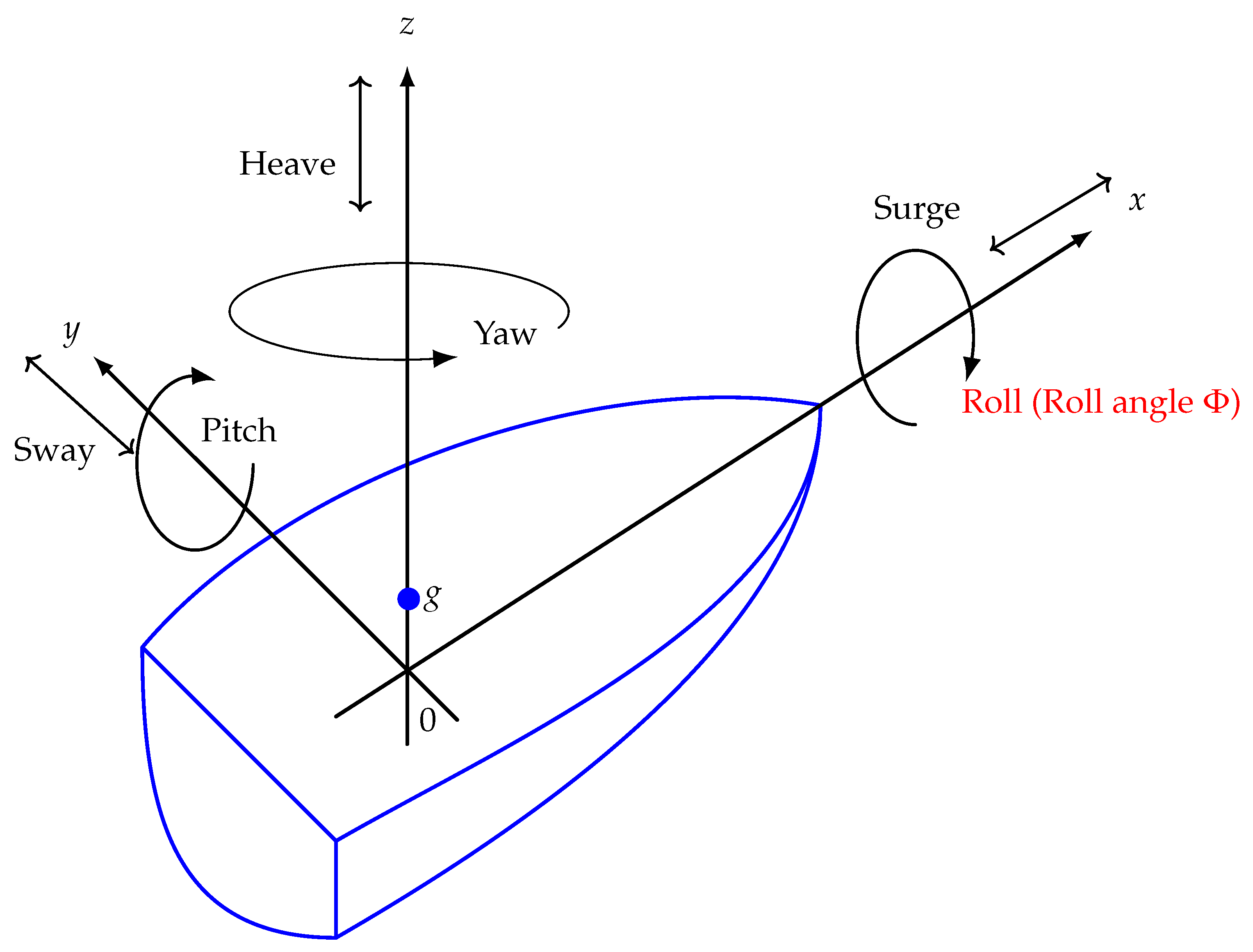
Figure 1. Schematic diagram of a ship with six degrees of freedom.
Mca 26 00033 g001
Figure 2. External Excitation Response Curve ( μ 3 = 2 , 5 , 15 and μ 1 = 0.4 , α 1 = 0.2 , α 3 = 1.5 , α 5 = 2 , σ = 30 , k = 1 and m 21 = 0.7 ).
Mca 26 00033 g002
Figure 3. External Excitation Response Curve ( μ 1 = 4 , 15 , 25 and α 1 = 0.2 , α 3 = 1.5 , α 5 = 2 , σ = 30 , k = 1 and m 21 = 0.7 ).
Mca 26 00033 g003
Figure 4. External Excitation Response Curve ( m 21 = 4 , 15 , 25 and μ 1 = 0.4 , α 1 = 0.2 , α 3 = 1.5 , α 5 = 2 , σ = 30 , k = 1 ).
Mca 26 00033 g004
Figure 5. ω 0 = 1 ; μ 1 = 3 ; m 21 = 0.7 ; μ 3 = 5 ; α 1 = 0.2 ; α 3 = 1.5 ; α 5 = 2 ; k = 1 ; f = 1 ; σ = 0.1 .
Mca 26 00033 g005
Table 1. Degrees of freedom for ship dynamics.
nAxisDirection of MotionSymbol
1translation along xsurgex
2translation along yswayy
3translation along zheavez
4rotation along xroll Φ
5rotation along ypitch ψ
6rotation along zyaw χ
Publisher’s Note: MDPI stays neutral with regard to jurisdictional claims in published maps and institutional affiliations.

