Abstract
Biological mapping of the visual field from the eye retina to the primary visual cortex, also known as occipital area , is central to vision and eye movement phenomena and research. That mapping is critically dependent on the existence of cortical magnification factors. Once unfolded, has a convex three-dimensional shape, which can be mathematically modeled as a surface of revolution embedded in three-dimensional Euclidean space. Thus, we solve the problem of differential geometry and geodesy for the mapping of the visual field to , involving both isotropic and non-isotropic cortical magnification factors of a most general form. We provide illustrations of our technique and results that apply to surfaces with curve profiles relevant to vision research in general and to visual phenomena such as ‘crowding’ effects and eye movement guidance in particular. From a mathematical perspective, we also find intriguing and unexpected differential geometry properties of surfaces, discovering that geodesic orbits have alternative prograde and retrograde characteristics, depending on the interplay between local curvature and global topology.
1. Introduction
Since ground-breaking work of Hubel and Wiesel [1], and Daniel and Whitteridge [2], consideration of mapping of the visual field from the eye retina to visual cortex has become increasingly relevant in psychophysics studies of vision in general and eye movements in particular. Daniel and Whitteridge showed that retinotopic mapping is critically dependent on the existence of cortical magnification factors [2]. Human or primate primary visual cortex, or occipital area , is of foremost concern. Daniel and Whitteridge also showed that has a convex three-dimensional shape once it is unfolded [2], a discovery confirmed by, and consistent with, other major investigations [3,4,5]. Our paper is premised on this pioneering work. We shall posit that unfolded can be modeled as a surface of revolution embedded in three-dimensional Euclidean space, at least with a certain degree of mathematical precision.
In many fields, the study of geodesy has always been and still is vital to the development of science, technology, and engineering. Geodesic curves are mathematically defined as parallel-transporting their own tangent vectors on any smooth manifold. Extremal paths connecting points on smooth manifolds are typically provided by geodesic arcs.
Pursuing general relativity studies [6,7,8,9], we developed geodetic procedures that result in first-order differential equations obeyed by geodesic curves over regular two-dimensional (2D) surfaces of revolution, S, embedded in ordinary three-dimensional (3D) Euclidean space, .
With the prospect of applications to vision and eye movement research, we provide in this paper an essential mathematical tool for any such application. That is a complete formulation and solution of the differential geometry and geodesy problem pertaining to conformal diffeomorphisms between the unit sphere, , representing the visual field, and surfaces of revolutions, such as . We consider both isotropic and non-isotropic CMF’s. Isotropic CMF’s are presumed to properly account for most experimental characterizations of . Non-isotropic CMF’s are required to account for stereographic projections to planar geometry or displays. Spheroidal geometry may also be formulated in terms of non-isotropic CMF’s and thus compared with the CMF-isotropic geometry of .
In this paper, we consider in particular the model framework provided in Ref. [2]. However, our geodetic technique applies generally to any regular surface of revolution, derived from a plane profile curve rigidly rotated around a z-axis, thus providing azimuthal symmetry. It produces first-order geodesic-orbit differential equations that can be readily solved by quadrature or numerical integration. Remarkably, we rely exclusively on ordinary calculus, rigorously bypassing any more substantive use of Ricci calculus. Most notably, our geodetic technique does not require any determination of Christoffel symbols for any surface of revolution.
No geodetic characterization of has been rigorously obtained heretofore. Our technique thus provides an essential tool for mathematical modelling and description of correlations between eccentricity and acuity among items in their representation. That is bound to be critical for studies involving visual ‘crowding’ effects [10,11,12]. Geodetic patterns and their analysis on may also critically inform studies of eye movement guidance in visual search [13,14,15,16,17,18,19,20,21,22,23,24,25,26].
2. Visual Cortical Surfaces
Physically, light rays from external sources pass through the eye’s lens system into the retina, a sheet of photoreceptor cells lining the curved inner surface of each eye. The visual axis (or line of sight) corresponds to the light ray that passes through the center of the pupil and hits the center of an area within the retina called the fovea. The fovea has the highest concentration of retinal receptors. The spatial density of ganglion cells, which receive visual information from photoreceptors and transmit it along the optic nerve, decreases in all directions from the center of the fovea. Consequently, the highest visual resolution occurs in the fovea and decreases peripherally with increasing visual angle.
The primary visual cortex, or area in the back of the brain, consists of a thin sheet of cells that, for our purposes, can be described as a 2D surface with a homogeneous and isotropic density of neurons. With good approximation, the projection of retinal units into , via the lateral geniculate nucleus, accomplishes a biological remapping that provides each retinal processing unit with an equal area of for further processing [27,28]. Consequently, the projection of dense foveal concentration of retinal receptors occupies a much larger proportion of than do more peripheral retinal regions.
Daniel and Whitteridge [2], described a cortical magnification factor (CMF) in terms of the number of millimeters () along meridians of concerned with one angular degree of ‘eccentricity’, w, in the visual field. Mathematically, one can model the visual field as the hemisphere of the 2D unit sphere, , having as colatitude, relative to the visual axis. Daniel and Whitteridge [2], found that the CMF decreases with increasing eccentricity w on , but the CMF hardly varies with the azimuthal angle of revolution around the visual axis. Subsequent research has confirmed those findings [3,5,10,29,30].
The CMF is an experimentally determined function. Since the total area of varies from individual to individual and from species to species, the CMF is individually peculiar, although it is commonly expressed as an average across adults of a given species.
In typical vision experiments, the minimum size that a symbol or a chart letter drawn on a screen must have in order to be recognized by an observer increases with eccentricity w in the visual field, away from the visual axis. The farther out, the bigger that chart letter must be drawn on the screen. The size threshold for perceptual identification is commensurate with the CMF. It means that, if we visualize threshold-sized letters on a screen as mapped on , each has about the same size on : see Figure 8. For the reverse situation, i.e., equally sized chart letters on a screen, their size as mapped into shrinks with increasing eccentricity, as shown in Figure 1 of Ref. [10].
With regard to measurements of distance between points on , previous numerical estimates could at best approximate geodetic separations at relatively short range, but hardly so for more distant points, lying on distant meridians of , for example. This problem provided our initial motivation to develop a mathematically rigorous method to perform geodetic calculations on at all distances, which is required to account for magnification of visual interactions throughout the entire mapping of items on from the visual field.
It has been previously demonstrated that physiological measures in other visual cortical areas and behavioral performance measures are invariant under relatively simple transformations of the configuration of stimuli as they are mapped in space [10,11,12,18]. This does not imply that those perceptual phenomena necessarily result from processing within . It does mean, however that eccentricity-dependent scaling is basically established by the CMF, as laid out in and then inherited by further connections with other cortical areas. It is thus plausible that spatially based perceptual phenomena may be further understood or revealed when studied directly within the representation of the visual field, which in turn requires a precise geodetic account of that mapping.
All such considerations essentially apply to a single fixation during which visual space is mapped from the eye retina to the primary visual cortex. Let us now consider the even more complex problem of the evolution of that mapping from one fixation to the next. Visual search generally proceeds through a series of eye movements consisting of saccades and fixations that bring sequentially different areas of the scene under scrutiny by the eye’s fovea. Affecting that pattern is a complex interplay between the scene’s display and boundaries and the observer’s perceptual, attentional, and mnemonic resources, whether deployed automatically or intentionally, overtly or covertly. Perceptual constructs such as the area of conspicuity (AC) or attentional focus, inhibition of return (IOR) or attentional momentum, scanpaths or other search strategies have been quantitatively investigated and further simulated with computational models [13,14,15,16,17,18,19,20,21,22,23,24,25,26].
Such research, however, is typically based on the externally fixed visual scene. The presence of cortical magnification implies that, after each saccade or eye movement, that visual scene is entirely transformed as remapped in the primary visual cortex, with its major accompanying changes in cortical object sizes and distances relative to other items originally present at each fixation. All such complex reconstructions derive from the biological remapping of the visual field to the primary visual cortex. Geodetic remapping of neighboring and distant items directly on a model surface may thus provide further insight into complex perceptual constructs such as AC, IOR or scanpath features, complementing investigations of visual search patterns and guidance based exclusively or primarily on the appearance of the external scenery.
The mapping of visual space on the primary visual cortex is suitable for an enlightening application of our general mathematical formulation of geodesy to diffeomorphic surfaces of revolution. This requires, however, a considerable degree of mathematical idealization and the following simplifying assumptions. We model the neural mapping as a conformal diffeomorphism between the unit sphere, , and its representation on . We must assume such diffeomorphism to be axially, i.e., azimuthally symmetric, since only that pertains to surfaces of revolution about that z-axis. We thus set aside for the moment some experimental evidence that further suggests somewhat different CMF’s along different meridians of , e.g., in the upper versus the lower visual hemifields [31]. We also assume that the left and right visual hemifields are seamlessly joined, ignoring their physical separation in the brain.
Beyond that, we consider an independent hypothesis of local isotropic magnification, positing locally equal magnification factors, latitudinally and longitudinally. That hypothesis is very restrictive, whereas it is not at all mathematically required in our geodetic theory. Thus, we will also provide more general equations and illustrations of diffeomorphisms that involve local anisotropic magnification, latitudinally and longitudinally. Nevertheless, for specific illustrations of geodesy on , we will focus on classical literature that makes the assumption of local isotropic magnification, using a basic expression of isotropic CMF with parameter values determined experimentally [2,5,10,29].
There have been, of course, many studies of neuroanatomy and modelling of visual cortex and retinotopy. Besides studies to which we specifically refer, other important works include those of Boscain, Bosking, Bressloff and Cowan, Citti and Sarti, Duits and Mashtakov, Hoffman, Petitot, Schwartz, Zucker, as quoted in Refs. [32,33,34,35,36,37,38,39,40], for example. Some of those studies apply analytic and differential geometry techniques comparable or superior to ours.
Let us consider, for example, the spherical extension of Mashtakov and Duits [40], of the Petitot–Citti–Sarti model [37,38,39]. Unlike the earlier planar approximation, the eye retina is approximated as a hemisphere, envisioned as a base manifold. A retinotopic map of to , involving a CMF, may then be modeled as a fiber bundle. More specifically, the lift of an image by the cortex can be interpreted as a map from , i.e., the retina, to , representing the cortex as a double cover of the group. Then, the Hopf fibration naturally appears as a fiber bundle, where the base manifold is and a fiber is : see Figure 4 in Ref. [40]. This construction allows for modeling the summation of the output of neural cells along vertical connections on , i.e., inside orientational hypercolumns, as a real-valued function. Introducing in this fiber bundle an appropriate sub-Riemannian manifold and metric, corresponding geodesics that obey certain variational principles of ‘cost optimization’ can be devised to approximate ‘perceptual completion’ of contours stored as neural information on [38].
Although there must ultimately be important connections, both the approach and the technique that we develop in this paper are quite different from those that we just mentioned. Here, we do not question nor investigate either the neurological structure or the perceptual reconstruction of the retinotopy. We just take at face value the model derived from Refs. [2,3,4,5]. Then, we solve mathematically the geodesy problem for that model, or any other surface of revolution, for that matter, generated from diffeomorphisms with any isotropic or non-isotropic CMF’s. It turns out that our exact solution of that problem technically circumvents any need of Ricci calculus, let alone any use of sub-Riemannian fiber bundle models designed to account for architecture and connections between cells [37,38,39,40], which we cannot investigate at this time.
3. From Ricci Calculus to Geodesic Orbits on Surfaces of Revolution
A two-dimensional (2D) regular surface of revolution, S, is generally obtained by rigidly rotating a one-dimensional (1D) smooth plane curve, , called the profile curve, around a coplanar z-axis [41]. The azimuthal angle of axial rotation and symmetry, , varies continuously between 0 and radians. For the sake of simplicity, we may further assume that the profile curve does not intersect itself.
It is natural to transform from Cartesian to cylindrical coordinates, , to identify points, , of the three-dimensional (3D) Euclidean space, , in which S is embedded. Namely,
We may set for all points lying on the profile curve, which is thus parametrized with values through coordinates . Then, upon revolution of , points on S can be identified in terms of values.
Now, the path of the profile curve may be obtained from elimination of the -parameter, which generates a functional relation between r and z. For our applications, it is convenient to express as that functional relation. Alternatively, we may derive . Under conditions for which the inverse function theorem applies [41], those relations are equivalent and we may assume that both the function and its inverse are locally single-valued. Globally, however, is more typically single-valued. As Figure 2 later exemplifies, there are typically two different z-values, one above and one below the equatorial plane that correspond to the same positive r-value.
In cylindrical coordinates, the infinitesimal arc element of Euclidean distance in is differentially derived from Equation (1) as
When points of are further constrained to lie on the 2D surface, S, the functional relation, , defining the profile curve path, requires that . That reduces the arc element along S to
where , summation is implied over repeated dummy indices and the metric tensor components are obtained as
In general, a smooth curve lying on S can be parametrized with values upon which its two coordinates depend, i.e., . Tangent vectors, , to on S thus have two corresponding components, .
A geodesic curve on S has this defining characteristics: it transports its own tangent vector, , with components, parallel to itself, as a curve parameter, , called affine, increases continuously. Intuitively, this means that a geodesic curve advances as ‘straight’ as it possibly can along the curved S surface. Typically, either an extremal or possibly the shortest arc length between two neighboring points on S is measured by a geodetic path connecting those two neighboring points.
Masters of the 19th and 20th centuries developed powerful mathematical theories of differential geometry on manifolds. Currently, we refer to some of that as Ricci calculus, providing rules to perform ‘absolute’ differentiation of tensor fields. In particular, geodesic curves are defined as having zero covariant derivative, meaning ‘no change’ of their tangent vectors along their advancing direction on the manifold. In other words, the tangent vector remains ‘covariantly constant’ along a geodesic curve on the manifold, implying ‘no intrinsic acceleration’ along it.
The basic differential equations obeyed by the contravariant components, , of the vector, , tangent to a geodesic curve, or, equivalently, by the coordinates, , of the geodesic curve, have the form
Given a vector basis, , for the expansion of vectors tangent to the manifold, Christoffel symbols, , represent the i-component of the covariant derivative of the basis vector along the basis vector [42]. Most notably, Equation (6) are second-order differential equations obeyed by the coordinates, which determine the geodesic curve, .
Introducing covariant vector components,
equivalent geodesic equations
can be generally derived [43]. Both forms of geodesic equations inherently define classes of affine parameters, , linearly related to each other.
When there are metric symmetries, Equation (8) is most suitable to provide corresponding conserved quantities. For surfaces of revolution S with axial, i.e., azimuthal symmetry, components are independent of : see Equations (4) and (5). Therefore, a first integration of a -component in Equation (8) yields immediately a conserved quantity
In a mechanical analog, Equation (9) represents conservation of angular momentum along the symmetry axis. In elementary differential geometry, the same result can be obtained more laboriously and it is known as Clairaut’s relation (1733, 1735) or theorem [41], which should not be confused with other important theorems due to Clairaut. Notice in particular that a geodetic curve profile or any other -meridian have zero ‘angular velocity’, hence .
Parallel transport by geodesic curves of their tangent vectors further requires conservation or constancy of the vector’s norm or length. For geodesics on S, we thus obtain
where Equation (9) has been introduced in Equation (3), divided by . In a mechanical analog, the positive constant plays a role similar to that of energy conservation. In particular, setting amounts to setting the curve affine parameter equal to the arc length itself, namely, .
Thus, without any need to further integrate either geodesic Equation (6) or Equation (8), we are able to express Equation (10) as a first-order decoupled differential equation
which can be directly integrated by separation of variables.
Surprisingly, elementary books in differential geometry remain ultimately stuck with Equation (6). As a result, Pressley [41], states on p. 227 that “geodesic equations for a surface of revolution cannot usually be solved explicitly.” Likewise, the opening paragraph of Sec. 7.6, p. 174, of Ref. [44] states that for “surfaces of revolution... it is usually still not possible to solve the geodesic equations explicitly...” In fact that is precisely what we can do, using Equation (11). Do Carmo arrives at a geodesic Equation (6) on p. 261 of Ref. [45] that is equivalent to our Equation (11). He does that by laboriously reworking through Christoffel symbols and Equation (6). That is redundant, in our opinion. Nevertheless, do Carmo’s derivation is certainly correct, formally, and further instructive, mathematically.
Further progress can be made by relating initial conditions to the study of turning points, having
Thus,
may provide a turning point of Equation (11). In a mechanical analog, such may play a role similar to that of a periapsis.
On the other hand, if vanishes for a greater -value that may provide either the actual turning point, as in Equation (28) of Ref. [7], or another turning point further away, which may then play a role similar to that of an apoapsis in a mechanical analog. The purple line, representing a geodetic equatorial parallel in Figure 1, provides an example of the latter, i.e., a ‘maximal apoapsis’.
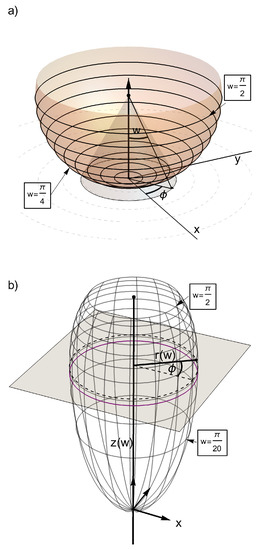
Figure 1.
(a) representation of the visual field hemisphere, , expressed in spherical-polar coordinates (w, ). The visual axis, having , is aligned with the z-axis, but it extends downward from the eye fovea position at , represented by the ‘visible’ dot at the center of . The eccentricity, w, is the colatitude referred to the visual axis, rather than the positive z-axis. The azimuthal angle, , spans the range counter-clockwise around the positive z-axis. Ten parallel latitudinal circles are shown, separated by equal increments of w from 0 to . Parallels are ‘geodetic circles’ but not geodetic curves, except for the equatorial great circle at ; (b) representation of the primary visual cortex, , in cylindrical coordinates (, , ). Surface parametrization is still made in terms of the eccentricity w and azimuthal angle in the visual field. However, the cortical location corresponding to the eye fovea is now set at the origin of cortical space, and the visual axis, still having , now coincides precisely with the positive z-axis of axial symmetry in . Ten parallel latitudinal circles are shown, separated by equal increments of w from 0 to . Parallels are ‘geodetic circles’ centered at the foveal origin in . Those parallels are not geodetic curves, however, except for the maximal equatorial parallel, colored in purple. The CMF has the form given in Equation (30) with parameter values of in units of millimeters and in units of inverse radians [5,29].
In terms of defined by Equation (13), by taking the ratio between first integrals in Equations (9) and (11) for , we can eliminate the presence of any affine parameter and obtain a geodesic orbit equation
This differential Equation (14) represents a central result of ours. It can be directly solved for any regular surface S of revolution by quadrature or numerical integration, virtually by-passing any more substantive Ricci calculus. Just like Equation (11), indeed, Equation (14) requires no determination of any Christoffel symbol for any regular surface of revolution!
Corresponding to Clairaut’s relation [41], we can also show that
is conserved along a geodesic. Here, represents the angle that a parallel-transported vector , tangent to the geodesic curve, forms with the local meridian, passing through a point at on S. Thus, parallel transport from an initial vector tangent to S at an initial point yields a geodesic orbit equation
Although differently parametrized, Equations (14) and (16) are equivalent via Equation (15). One may use one geodesic orbit equation or the other, depending on one’s choice of initial or search conditions.
Furthermore, Equation (12) means that is an extremal point. Correspondingly, Equation (15) implies that, at , we must have , meaning that a geodesic orbit must become extremally tangent to a local parallel at a minimal turning point. Parallels themselves are not geodetic, however, with the following exception. When becomes also extremal, we have and in Equation (4). That generates a geodetic equatorial parallel, reducing Equation (11) to a maximal turning point: . The purple line in Figure 1 provides an example of that ‘apoapsis’.
If one wishes to use a typically single-valued function to globally define the profile curve, the geodesic orbit equation, corresponding to Equation (14), becomes
where
and
Typically, is unique, while may or may not be. For example, on an ellipsoid of revolution with a geodesic equatorial circle in the plane of reflection symmetry, typical geodesics wind around an equatorial band, cycling between its two symmetrically opposite bounds, or ‘vertex latitudes’, derived from the same minimal value [46]. On each cycle, these typical geodesic curves also cross twice the maximal equatorial value, at ‘nodes’ where is correspondingly minimal on account of Equation (15).
Let us also recall that fundamental second-order differential ‘equations of motion’ such as Equation (6) or Equation (8) do not explicitly contain any initial conditions or parameters. Our first-order differential equations explicitly contain conserved quantities that reflect initial conditions or parameters, such as L, C, or because they already involve first integrations of more fundamental ‘equations of motion’.
4. Geodesy on the Primary Visual Cortex and Diffeomorphic Surfaces of Revolution
In our mathematical formulation, we use cylindrical coordinates to describe as a surface of revolution embedded in 3D Euclidean space, . We consider the 2D unit sphere , parametrized in spherical-polar coordinates. When we refer to the visual field more specifically, we limit to the range of the visual angle or ‘eccentricity’, but let us still denote as the corresponding 2D unit hemisphere. Now, we wish to construct a magnified conformal diffeomorphism from to , which we denote as .
Most generally, latitudinal and longitudinal dilations of from involve arbitrarily different and magnification functions. However, azimuthal or axial symmetry requires that both latitudinal and longitudinal magnification functions become independent of . Since in this paper we are dealing exclusively with surfaces of revolution, we shall assume that -independence.
Vice versa, loss of axial symmetry requires consideration of metric symmetries that may still exist. Triaxial ellipsoids provide a prototypical example [46]. Jacobi famously discovered (1839) that geodesic equations, expressed in ellipsoidal coordinates, are still separable, although it was later proved by Cohn-Vossen that there are no Killing vector fields for smooth convex surfaces embedded in . That would also be the case if there are different CMF’s along different meridians of , e.g., in the upper versus the lower visual hemifields [31].
Setting that aside, we assume a latitudinal CMF such that
Thus, parallel circles on have circumferences of length , corresponding to parallel circles on with circumferences of length .
Since azimuthal symmetry also requires that all meridians must be equally magnified longitudinally, an arc length along any meridian on is mapped to an arc length along the corresponding meridian on , involving such a longitudinal CMF at any given w.
Now, local isotropic magnification generally means that . Thus, assumptions of azimuthal symmetry and local isotropic magnification are completely independent conditions, neither necessary nor sufficient to each other. Since in this paper we always require azimuthal symmetry, making the further assumption of local isotropic magnification implies the existence of a single isotropic cortical magnification factor such that
Such restrictive assumption is inessential to our mathematical formulation, as Equation (27) will demonstrate. Nevertheless, we will make the assumption of Equation (21) when referring to classical experimental studies on the primary visual cortex [2,3,5,10,29,30]. Other studies, however, have considered possibilities of non-isotropic cortical magnification and proposed alternative models and expressions for corresponding CMF’s [32,33,34].
While the arc element on is expressed as
the arc element on can be derived from that of Equation (22) by using Equations (2) and (3). Assuming local isotropic magnification, Equation (21), we thus express the arc element on in terms of coordinates on as
where
Originally, Rovamo and Virsu illustrated such a mapping in Figure 1 of Ref. [29]. We reproduce their results and the essential features of the diffeomorphism in our Figure 1.
Given Equation (24), Equation (23) corresponds to Equation (3), to which our general geodesic results apply. Using Equations (13) and (14), we may then express the geodesic orbit equation on as
This first-order differential equation represents our main result for application to , assuming an isotropic CMF of general form. Here, the conserved quantity is the minimal value at a turning point. According to Equation (15), we may equivalently replace with at the initial point.
It is straightforward to derive a generalization of the geodesic orbit Equation (26) that does not require the assumption of isotropic magnification, as expressed in Equation (21). All we need to do is to replace for in Equation (24) and for in Equation (25), according to the more general latitudinal CMF representation of in Equation (20). Thus, following the same procedure that led us to Equation (26) for isotropic magnification, we obtain for non-isotropic magnification that
These first-order differential equations can be directly integrated by separation of variables. Assuming that the coordinates of the initial and final points have and , a geodesic orbit with develops. If we take the positive square root of Equation (26), the unknown angle of the final point is given by
Being expressed as an integral area, Equation (28) provides a complete solution by ‘quadrature’ of the differential Equation (26). However, Equation (28) applies only when no turning point is traversed by the geodesic arc that connects the two points. An alternative expression will be given later in Equation (34) when a turning point must be traversed along the way.
Depending on the functional form assumed for , it may or may not be possible to further express Equation (28) in terms of special integrals of mathematical physics that are currently provided as standard functions in computer algebra packages. That was the case for similar work of ours [7], involving Jacobi elliptic integrals and functions [47,48]. That is not so for the form of most basically considered in vision research [2,3,5,10,29,30]. Nevertheless, accurate solutions of Equation (28) can always be obtained numerically, as we will demonstrate in Section 5. Particular care must be taken, however, if a minimal turning point at is attained because the integrand in Equation (28) diverges therein, although numerical integration must still converge.
It is instructive at this point to check the structure and verify the correctness of Equation (28) by reproducing geodesic orbits on , which must be arcs of great circles. Of course, we can do that by simply setting in Equation (28). That integral can now be performed analytically, yielding
The integrand and its result are indeed real in the region of integration, where . Any great circle on correspondingly cycles between two parallel circles symmetrically placed above and below the equator, becoming tangent to such ‘vertex latitudes’ with minimal distance of closest approach to the z-axis.
We have also reproduced classical results for geodesics on ellipsoids of revolutions [46], by integrating Equation (27) with spheroidal non-isotropic CMF’s, expressing such quadratures analytically in terms of Jacobi elliptic integrals and functions [47,48].
Experimentally, it has been found that the cortical magnification factor is basically isotropic and monotonically decreasing with w. A basic expression for
has been provided and variously parametrized [2,3,5,10,29,30].
The CMF, hence A in Equation (30), is a length measured in , while in Equation (30) must be a pure number, to maintain unit coherency. Trigonometric functions and corresponding calculus operations are most readily performed by measuring angles in radians. As we do that, B in Equation (30) must be expressed in units of the inverse of a radian. After calculus operations are completed, angular w-values may also be converted to degrees by multiplication. In that case, numerical B-values must be correspondingly converted by a 57.2958 division. We typically consider all w-values between 0 and radians in the visual field, though a zone of particular interest experimentally lies below w-values of about radians or 9 degrees from the center of the fovea: see Figure 1.
The curve profile for the surface of revolution can be obtained by combining Equation (4) with Equation (24) to yield
The right-hand side of Equation (31) must be expressed exclusively as a function of eccentricity, taking the w-derivative of from Equation (25). After integration of the positive square root of Equation (31), the curve profile can be expressed parametrically in terms of w as .
Any arc length along the curve profile or any meridian is immediately obtained by analytic integration of Equation (30), yielding
where log denotes the natural logarithm.
In Figure 2, we plot the curve profile for as given in Equation (30), using parameter values of and for rhesus monkeys [5,29]. Alternative values can be found in the literature, e.g., and for humans [10,30].

Figure 2.
Curve profile corresponding to any meridian () shown in Figure 1b. Here, the z-axis is drawn horizontally and measured in . The r-axis is drawn vertically and also measured in . Here, eccentricity w-values are converted to degrees, whereas they are expressed in radians in Figure 1b. The geodetic equator therein is marked here by two purple-dot intersections that lie at . Consequently, the positive function is single valued, whereas its inverse, , is double-valued. Thus, the former relation accounts more globally for this curve profile. Only non-negative r-values are attributed to the curve profile, which is then cylindrically rotated around the z-axis. and .
Upon revolution, the shape of the surface, as shown in Figure 1b, is qualitatively similar to that of a spheroid, for which analytic solutions of geodesic orbit equations can be obtained using either our technique or traditional methods. Thus, geodesics on share some global or qualitative similarities with geodesics on spheroids [46]. However, lacks the reflection symmetry about the equatorial plane that spheroids have. More critically, the negative slope of that persists at for the particular form of Equation (30) is responsible for an infinite Gaussian curvature at that umbilical point singularly. To smooth that out, should at least be rounded as to attain a zero-derivative at . Based on available experimental evidence, we have no particular reason nor means to meaningfully remove the cusp of at the foveal point that is responsible for the umbilical singularity of , assuming Equation (30). This means that geodesics on that reach to very low w eccentricities, rather than the foveal origin exactly, may display some peculiar behavior therein. This must be examined with even greater numerical accuracy in the integration of Equation (28) when small or vanishing values are attained.
Parallel latitudinal circles are not geodetic on , except for the equatorial parallel. That can be determined by setting to zero ) derivatives of the left- and right-hand sides of Equation (26), respectively. Equivalently, one may set to zero the derivative of the square-root of Equation (25), thus determining the largest turning point, . For the form assumed in Equation (30) with our chosen parameters [5,29], we obtain . In Figure 1 that geodetic equator, colored in purple, lies a bit below the third parallel circle up from the bottom, which has .
5. Illustrations
In principle, we have thus solved completely the problem of geodesy on surfaces of revolutions in general and on a basic model of the primary visual cortex, or area , in particular. In this section, we perform some numerical integrations of our central differential equations and we generate corresponding illustrative figures. These integrations and figures are meant to demonstrate as simply as possible our mathematical techniques and further depict main features of geodesics on models of the primary visual cortex, visual field and their stereographic projections, all connected by various types of axially symmetric conformal diffeomorphisms. Such illustrations are not meant to be either exhaustive nor predictive of any specific visual phenomenon or experiment. At this stage, our geodetic techniques have been developed with the purpose of providing a basic tool to further investigate any such phenomenon and develop a deeper understanding or more advanced theories of vision.
In Figure 3a, we show an example of a geodesic orbit on a model of , based on the isotropic CMF given in Equation (30). That geodesic orbit connects a red point at coordinates (, ) with a blue point at coordinates (, ). In order to find the geodesic arc that connects those two points, we must solve a so called ‘inverse geodesic problem’. Namely, we must find the ‘right’ tangent-vector direction at the red point, in terms of conserved or quantities in Equation (15), which sets the geodesic on a course that arrives ‘ballistically’ at the intended destination. To that end, we use a root solver program that finds through converging iterations. Namely, we vary time and again after numerical integrations of Equation (28) until a geodesic orbit starting at (, ) arrives precisely at (, ) ultimately. In this example, the sought parameter value is . Given Equations (15) and (25), we have equivalently and radians degrees at the red point.

Figure 3.
(a) example of a geodesic orbit on connecting a red point at coordinates (, ) with a blue point at coordinates (, ). A root solver program finds that or degrees for this geodesic orbit; (b) diffeomorphic image of the same geodesic orbit on stereographically projected from the visual field to its tangent polar plane at . and .
This geodesic orbit wraps around along the shortest path between the red and blue points, as a string pulled tight against a physical realization or 3D printing of the surface would. We should mention, however, that there are infinitely many more geodesic orbits that also connect the same two points. All those geodesic orbits still parallel-transport their own tangent vectors, but wind around any number of times. Similar results for spheroids, paraboloids, hyperboloids, and other quadric surfaces of revolutions further depend on characteristics of their global topology [7].
Notice that in this example. This means that the ‘vertex latitude’ of this geodesic lies beneath or ‘south’ of the ‘launching’ red point. After its northbound ‘launch’ with , the geodesic crosses the equatorial parallel at a ‘node’ with its smallest radians at . The final blue point also lies beneath or ‘south’ of the other northern ‘vertex latitude’, where this geodesic would become again tangent to a parallel having the same minimal radial turning-point value. However, the geodesic arc that connects the red and the blue points never reaches any minimal turning point at either of those ‘vertex latitudes’ in Figure 3a.
In Figure 3b, we show the diffeomorphic image through of the same geodesic orbit on stereographically projected from the visual field to its tangent polar plane at . On , the geodesic arc that connects the red with the blue point is of course a Euclidean straight segment. That illustrates most vividly how profoundly different are geodesic arcs that connect distant item representations either on or their projecting images on a flat screen. Mathematical details on how to perform the precise stereographic projection, , which is required for visual representation of a plane screen are provided in Appendix A, which may be read at this point.
In Figure 4, we show the explicit construction in 3D of the stereographic projection from onto its tangent polar plane , resulting in the mapping of the original geodesic curve on to its ultimate image on the plane . Neither of the -geodesic-curve images on and are geodetic in those latter two manifolds: starkly far from geodetic in fact.

Figure 4.
3D construction of the stereographic projection from onto its tangent polar plane including the image on of the geodesic orbit on shown in Figure 3a. The eye position is at the projection center of . Gray lines (virtually corresponding to light rays) show the projection through the curve image on to the curve on the polar plane shown in Figure 3b. Notice that neither of the -geodesic-curve images on and are geodetic in those latter two manifolds: starkly far from geodetic indeed.
Now, suppose that, in Figure 3a, we steadily lower the eccentricity of the blue point. The value must correspondingly increase, until it matches precisely . Then, the red point has become a turning point. That occurs for and . We may lower even further the eccentricity of the blue point. Then, we expect the value to decrease once again, as the geodesic ‘launched’ from the red point must initially ‘dip’ southward with , then reach its turning point at , before climbing again northward and ultimately reach the blue point. In this situation, the negative square root of Equation (26) for the first branch of the ‘dipping’ geodesic must be taken, whereas the positive square root of Equation (26) must still be taken for the subsequent climbing branch of the geodesic. Thus, Equation (28) must be replaced by
Ultimately, the eccentricity of the blue point may decrease to equate . In that case, the turning point lies along the meridian that bisects the latitudinal arc that now connects the equilatitudinal red and blue points. In that case, we find that or . In fact, symmetrically, at the blue point has the same sine as at the red point, i.e., 0.99183.
In all cases where the geodesic must first ‘dip’ south and traverse a turning point in order to ultimately connect two distant points, it is necessary to break the solution of the ‘inverse geodesic problem’ into two parts, smoothly connecting the two arcs that separately join the initial and final points to the same turning point. The root solver technique that we have outlined with regard to the drawing of Figure 3a can still be applied to both terms in Equation (34) with no fundamental change. Indeed, only a single parameter requires a ‘root solution’, since and in Equation (34) are related via Equation (25). For any two points initially given, it is relatively simple to determine first of all whether Equation (28) or Equation (34) should apply. Complete and efficient numerical solutions of this ‘technical’ problem are of great ‘practical’ concern, since data from psychophysics experiments may contain hundreds or thousands of items having similar eccentricities near the fovea. We have further generated routines that automatically find the geodesic arc connecting any two points, lying either below or above the geodesic equator, involving whichever ‘southern’ or ‘northern’ vertex latitude that may be traversed at turning points.
There are various alternatives to approach this type of problems most generally. Consider, for example, a ‘cluster’ of items on and suppose that you wish to determine with a given accuracy their geodetic distances from an initial point, , outside that ‘cluster’, say. You may then ‘launch’ from the corresponding a geodesic Equation (16) with any that generally ‘aims’ at the cluster. Then, by increasing and decreasing by multiples of a small increment, , you may generate a family of radial geodesics, all emanating from the same initial point that covers the cluster, ‘from side to side’. You can then generate another family of ‘geodesic circles’, orthogonal to the radial geodesic family, according to a Gauss Lemma [41,45]. You may thus cover the whole cluster with this coordinate-grid patch. Depending on the size that items may have on , you may refine your grid until each item tightly fits within a single or just a few quadrangles of your grid. The radial length from that quadrangle on to the initial point thus provides with good approximation the geodetic distance of its item from the original point. This procedure can be very effective and easy to program, since it does not require solution of any ‘inverse geodesic problem’. Notice, however, that geodesic ‘angular’ distances between items within the clusters are not provided by geodesic-circle arcs, since those are not geodesic curves. Of course, there are other ways to generate ‘normal coordinate’ patches that are fully geodesic [41,42,45], but those are more elaborate and may or may not be needed for ‘practical concerns’ on .
In Figure 5, we show the explicit construction in 3D of the stereographic projection on of the geodesic arc of great circle on , connecting the red point with the blue point. This projection is a Euclidean straight segment, i.e., a geodesic path on , mapping a geodesic path of great circle on through a geodesic diffeomorphism .
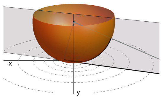
Figure 5.
Geodesic arc of great circle on and explicit construction in 3D of its stereographic projection to the tangent polar plane , resulting in the straight segment connecting the red and blue points in Figure 6a.
In Figure 7a, we draw two geodesic circles on , both centered at the point (, ). Their geodetic radii have lengths of 5 and 10 units (mm). In addition, geodetic ‘spokes’ of equal length are drawn for each circle. In the stereographic projection of the visual field on , shown in Figure 7b, images of three geodesic circles, having originally geodetic radii of 5, 10, and 20 units on , show their increasing distortion caused by the lack of isometry in their composite mapping.

Figure 7.
(a) two geodesic circles of radii 5 and 10 units (mm) centered at the point (, ) on . Radial geodesic ‘spokes’ of equal length are shown for each circle; (b) three geodesic circles of radii 5, 10, and 20 units on stereographically projected on . Their center point is shown in red. and .
In Figure 8a, we begin by drawing on four geodesic circles with equal radii of five units, arrayed tangentially to one another along the meridian. Thus, the areas of these four circles are approximately equal on . In Figure 8b, we first show the stereographic projections of these four circles on mapped with through the visual field to the plane. Images of the circle centers on are marked as red points on . Thus, geodesic circles with equal radii and approximately equal areas on map as increasingly magnified areas of stretched circles on as their visual eccentricities increase, as prescribed by cortical magnification. Further explanations of the lettering and corresponding surface orientations through stereographic projections are provided in Appendix B.

Figure 8.
(a) geodesic circles of radius 5 tangent to each other and centered along the meridian on ; (b) stereographic projections of the four circles to the plane. Scripts of the first four letters of the alphabet are inscribed inside the circle images on . Their inverse diffeomorphic images are mapped back to the surface to illustrate surface magnification and orientability. and .
Last but not least, we solve some cases of a ‘direct geodesic problem’ with remarkable consequences. Consider a geodesic starting at a turning point with a pre-assigned value, for example. According to Equation (25), an initial point at coordinates (, ) has that value. This initial turning point is marked by a ‘fat’ red dot in Figure 9. By parallel-transporting its own tangent vector from there on, we develop the unique geodesic orbit that solves Equation (28) through a continuum of final points (, ), all covariantly evolved from that initial red point with those initial conditions. The first semi-cycle of the geodesic, drawn in red in Figure 9, thus begins tangentially at the ‘southern vertex latitude’ and arrives tangentially at the ‘northern vertex latitude’. The second semi-cycle of the geodesics, drawn in green in Figure 9, does the converse, arriving again tangentially at the ‘southern vertex latitude’. However, the geodesic orbit has advanced longitudinally through this full cycle by an angular increment of radians, relative to the initial red-point angle . The third semi-cycle of the geodesic, drawn in purple in Figure 9, climbs northward just as the first semi-cycle did, while maintaining the same angular shift of all along, relative to the first semi-cycle. That shift is maintained at the ‘northern vertex latitude’, where the ascending purple line becomes blue, turning southward in its fourth semi-cycle. That blue line then arrives tangentially at the ‘southern vertex latitude’ with a longitudinal shift of , marked by a ‘fat’ blue dot in Figure 9, relative to of the initial red dot. After that, the geodesic orbit will advance indefinitely through rigidly shifted cycles, unless is exactly commensurate to , in which case the geodesic will become a closed periodic orbit. Typically, however, our open geodesic orbit will fill the entire band between its two ‘vertex latitudes’. This prograde geodetic shift, i.e., further advancing in the geodesic direction, is similar to that occurring on prolate ellipsoids [46]. This is of course a direct consequence of azimuthal symmetry. It is also worth noting in Figure 9 that crossings between geodetic branches accumulate around the ‘vertex latitudes’, where those branches become more and more latitudinally tilted.

Figure 9.
Two cycles of a prograde geodesic orbit bound between two ‘vertex latitudes’ that have the same distance of closest approach to the axis of symmetry, with a turning-point value of and a positive shift . Consecutive semi-cycle arcs of the geodesic are colored in red, green, purple, and blue, sequentially. and .
However, a more complex pattern of longitudinal shifts emerges on . Namely, there is a critical turning-point value, , for which and the geodesic orbit closes precisely after one cycle between ‘vertex latitudes’. No such kind of closed orbits exists on spheroids. A critical closed geodesic orbit is shown in Figure 10.

Figure 10.
Critical closed geodesic orbit with two turning points at ‘vertex latitudes’. and .
For , the longitudinal shift is positive, or prograde, as shown in Figure 9 for and in Figure 11 for , more extensively. However, for , the longitudinal shift becomes negative, or retrograde, i.e., lagging behind along the geodesic direction, as shown in Figure 12 for . That behavior is similar to longitudinal deficits of geodetic cycles occurring on oblate ellipsoids [46].
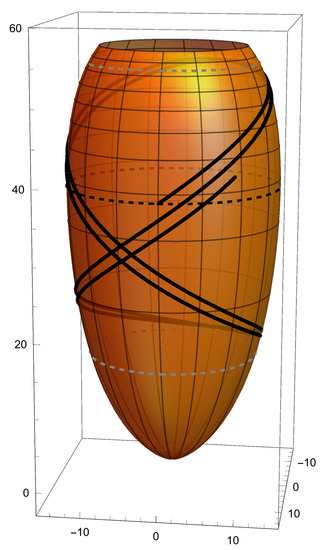
Figure 11.
Prograde geodesic with turning points at . This geodesic starts as northbound at the equator, marked by a black-dashed latitude. Two more crossings of the equator are shown, each advancing by a positive shift of . and .

Figure 12.
Retrograde geodesic with turning points at . This goedesic starts as northbound at the equator, marked by a black-dashed latitude. Two more crossings of the equator are shown, each lagging behind by a negative shift of . and .
This complex behavior originates from the interplay between local curvature and global topology, which is more complex on isotropically magnified surfaces than it is on equatorially symmetric spheroids. We shall not pursue any more advanced inquiry on this matter. Current computer packages allow extremely fast and accurate numerical integration of ‘simple’ equations such as Equation (28) for all cases of ‘practical’ concern, such as ours in this paper. However, further analytic characterization of primitives of Equation (28) for isotropically magnified surfaces may lead to discoveries of deeper connections with, or generalizations of, beautiful theories such as those developed for elliptic integrals and functions [47,48].
6. Conclusions
During foveation and an eye fixation, the probability of detecting a peripheral target is a function not only of target eccentricity, but also of the proximity of distracting objects from that target, which contributes to a ‘crowding’ limiting condition [11,12]. Visual crowding derives from the breakdown of one’s ability to identify peripheral objects in the presence of other nearby objects. In turn, this critically depends on cortical magnification of the visual field in the primary visual cortex, or area [2,3,5,10,27,28,29,30].
Following eye movements, mapping of items just recorded on the eye retina must be sequentially updated in a coordinate frame intrinsic to . Studies of vision or visual search did not possess heretofore precise mathematical tools, hence the ability, to take into account cortical magnification directly based on the representation of the visual field. Geodesy on was surmised, but hardly computable within a rigorous and complete mathematical framework.
In this paper, we have provided that framework and all the basic tools of differential geometry and geodesy that are needed to analyze and compute whatever pertains to any model of as a surface of revolution and its corresponding projections.
In Section 2, we summarized basic elements of retinotopy of the visual field on the primary visual cortex, emphasizing the cortical magnification involved in that biological mapping. We referred (a) to ‘crowding’ effects and (b) to constructs involving perceptual, attentional and mnemonic resources that guide or inform vision or visual search performed with eye movements and fixations.
Based on general relativity studies, we further developed our geodetic technique that applies to any regular surface of revolution embedded in Euclidean space. That leads to first-order differential geodesic equations that can be solved by quadrature or numerical integration. We rely exclusively on ordinary calculus, bypassing any more complex use of Ricci calculus and Christoffel symbols. A geodesic orbit first-order differential Equation (14) represents a central result that we provide in Section 3.
In Section 4, we applied our geodetic technique to a conformal diffeomorphism that represents the mapping of the visual field, represented as the unit hemisphere, , into , as illustrated in Figure 1. A geodesic orbit first-order differential Equation (26) provides our main result for application to surfaces of revolutions, expressed in terms of isotropic cortical magnification factors, or CMF’s, having a most general form. Integral solutions are provided in Equations (28) and (34) and applied to a CMF, Equation (30) that is typically considered in vision research.
The study of turning points is central to our geodetic formulation and the classification of geometries to which it applies. We applied that study particularly to the elliptic-like geometry to which belongs. ‘Direct’ or ‘inverse geodesic problems’ are thus formulated in terms of the prescription or search of a minimal parameter upon which our geodesic orbit solution in Equation (28) most critically depends. That is in turn related to initial conditions and consequent conservation of an angular momentum analog prescribed in Equation (15), corresponding to a theorem of Clairaut.
Most generally, latitudinal and longitudinal dilations of diffeomorphisms from involve different magnification functions. However, axial symmetry requires both latitudinal and longitudinal magnification functions to be independent of the azimuthal angle . We must assume that symmetry, since we are dealing exclusively with surfaces of revolution in this paper.
A further assumption of local isotropic magnification requires equality of latitudinal and longitudinal CMF’s. That is a very restrictive assumption, which is inessential in our mathematical formulation. Thus, we provide a generalized geodesic orbit Equation (27) that may apply more broadly in vision research. Besides that, Equation (27) is definitely needed to account for geodesy of general diffeomorphisms between the unit sphere and all kinds of surfaces of revolution, including spheroids and stereographic projections.
In practice or experiment, items may appear to be, or they are actually located or depicted on a flat surface or screen. We thus studied a corresponding stereographic projection of the visual hemisphere onto its tangent polar plane. That geodesic diffeomorphism maps geodesic paths of to geodesic paths of , but in terms of non-isotropic CMF’s. We provided more technical details of this type of stereographic projection and other diffeomorphisms involving non-isotropic CMF’s in an Appendix A. Further details regarding surface orientations and their preservation through stereographic projections have been provided in an Appendix B.
In Section 5, we presented and discussed various prototypical illustrations of our geodetic results on diffeomorphic surfaces , and their tangent plane. Those include solutions of ‘inverse’ and ‘direct’ geodesic problems with corresponding magnifications (see Figure 3, Figure 4, Figure 5, Figure 6 and Figure 7), projections of right-handed sides of orientable surfaces (see Figure 8), and cycling of either space-filling or periodic geodesic orbits between their ‘vertex latitudes’, with either prograde or retrograde longitudinal shifts on (see Figure 9, Figure 10, Figure 11 and Figure 12). Deeper connections between primitives of Equation (28) and theories of elliptic integrals and functions may emerge from these findings.

Figure 6.
(a) geodesic stereographic projection on of the geodesic arc of great circle on connecting the same red point at coordinates (, ) with the same blue point at coordinates (, ); (b) diffeomorphic image on of the geodesic arc of great circle connecting the red and blue points on the visual field. and .
We did not report in this paper further results regarding, for example, geodesic curvature, normal curvature, or relative torsion of general curves on . Nor did we present calculations of principal curvatures or other differential geometry characteristics of . In fact, our technique allows either analytical expression or accurate numerical evaluation of any such quantity, as well as precise calculation of any length or area of whatever figure on .
Both in principle and in practice the problem of differential geometry and geodesy on or any other surface of revolution with either isotropic or non-isotropic cortical magnifications from is thus fundamentally solved or soluble with our techniques.
This provides mathematical and computational tools to investigate to which extent geodesy may biologically affect or perceptually inform reconstruction of visual scenery in certain brain areas or connections. Of course, this is only an entry point to a wide range of inquiries that lie beyond the scope of this paper. However, there are at least some indications that a geodetic account of cortical magnification of the visual field from the eye retina to the area is a prerequisite for a more quantitative account and understanding of visual ‘crowding’ effects. Further questions of guidance of eye movements and fixations may also be better understood when grounded on a geodetic account of the sequential mapping of the visual field, beyond mere consideration of the external scenery.
Author Contributions
L.G.R. developed the basic theoretical formulation and mathematical solution of the problem. N.A.M. developed the computational implementations. N.A.M. generated all figures for the paper. L.G.R. wrote the original draft and final version of the paper. Both authors have read and agreed to the published version of the manuscript. All authors have read and agreed to the published version of the manuscript.
Funding
We acknowledge technical and financial support from the Vitreous State Laboratory at the Catholic University of America.
Acknowledgments
Brad C. Motter (BCM) of the Veterans Affairs Medical Research Program at SUNY suggested this problem. BCM summarized literature in vision research most relevant to this paper. We used some of BCM’s reviews especially in Section 2. We are deeply indebted to BCM for countless most productive discussions and his determining contribution to our work.
Conflicts of Interest
The authors declare no conflict of interest. The funders had no role in the design of the study; in the collection, analyses, or interpretation of data; in the writing of the manuscript, or in the decision to publish the results.
Abbreviations
The following abbreviations are used in this manuscript:
| CMF | cortical magnification factor |
| AC | area of conspicuity |
| IOR | inhibition of return |
Appendix A. A Stereographic Projection
In practice or experiment, items may appear to be, or they are actually located or depicted on a flat surface or screen. We may represent that, as a stereographic projection of the visual hemisphere onto its tangent polar plane, , at . Such mapping is depicted in Figure 5. With our coordinates, a straight line from the center of , where the eye is located, to a point on , where an item is located, intersects at a point .
The profile curve of has , and the arc element of is represented as
Now, a diffeomorphism is said to be geodesic if it maps geodesic paths, or ‘pre-geodesics’, of one manifold to geodesic paths of the other manifold. Our stereographic projection is a geodesic conformal diffeomorphism. Indeed, any plane through its center, , intersects the hemisphere along an arc of great circle and it then intersects the polar plane along a corresponding straight segment. Those intersections evidently provide diffeomorphic geodesic path images between the two manifolds: see again Figure 5. Only surfaces of constant Gaussian curvature can be mapped through geodesic diffeomorphisms, as shown in a consequential theorem of Beltrami that applies to our case: see Section 10.4 of Ref. [41].
By comparison of Equation (A1) with Equation (22), it is clear that is not related to by a single isotropic magnification factor. With the stereographic projection, meridians of are dilated to straight lines in by a longitudinal CMF, , whereas parallel circles of are dilated to concentric circles in by a smaller latitudinal CMF, . On the contrary, our basic diffeomorphism is isotropically magnified, but it is not geodesic. Neither nor is an isometry, since neither diffeomorphism preserves lengths. Our main concern is the composite diffeomorphism , which is neither isotropically magnified nor geodesic nor isometric. See Figure 3 and Figure 4, for example.
Our generalized geodesic orbit Equation (27) can be applied to the stereographic projection, setting and . That can be solved analytically, yielding geodesics on that are Euclidean straight lines, having minimal distance from the origin of , tangent to at .
Geodesic orbits on ellipsoids of revolution can be obtained by solving directly our Equation (14), based on coordinates. They can also be obtained more simply than classically by setting up conformal diffeomorphisms with , mapped with the same coordinates. To those diffeomorphisms our Equation (27) applies. For example, by inscribing in a prolate ellipsoid of revolution with axes , appropriate CMF’s are and . In this context, we may not report on such interesting mathematical developments. Recall, however, that differs from spheroids in one fundamental respect, namely that is isotropically magnified locally relative to , whereas spheroids are not so, thus profoundly differing in local curvature.
Let us also mention that the stereographic projection that we consider, , differs substantially from other stereographic projections, including the more common that joins a north pole of with all points on its equatorial plane, . That maps great circles on the entire onto circles of . Thus, is a conformal diffeomorphism that is not geodesic [41,49].
Appendix B. Surface Orientations through Stereographic Projections
In order to illustrate how surface orientations are maintained through stereographic projections, we inscribe scripts of the first four letters of the alphabet inside the four circle images on in Figure 8b. We know that geodesic segments on are Euclidean. Thus, we draw each letter script with polygonal lines joining 500 equally spaced points on . As a result, each letter script on may be regarded as a ‘fine-grained piecewise-geodesic composite’. Now, using the inverse diffeomorphism , we map these letters back to the surface in Figure 8a. Since curvature is a second-order effect locally, the letter scripts appearing on remain approximately ‘fine-grained piecewise-geodesic composites’ therein. The principle of this inverse diffeomorphic mapping is the same as that applied in Figure 6. The major difference is that, rather than joining two distant points, we connect multitudes of nearby points in each letter script drawn in Figure 8, thus roughly maintaining ‘letter-geodesy’ on both and .
Our readers will immediately notice that letter scripts mapped back from to appear as mirror-reflected in Figure 8a. This draws immediate attention to issues of orientability of our surfaces and stereographic projections that connect them. Indeed, all three , , and surfaces are orientable and internally oriented, [41,42]. We must then decide how to choose ‘right-handed’ or ‘positive’ sides that map consistently between those three surfaces. Our letters are first written on the plane while looking down from the z-axis. Correspondingly, we define the ‘positive’ sides for all three surfaces as those that face increasing z-values along that symmetry axis. Then, the ‘positive’ sides of and are those that face the interior of those two surfaces, corresponding to the ‘upside’ of the plane. Indeed, that becomes the ‘inside’ of the surface if it is homeomorphically deformed as to surround the positively increasing z-axis. Consequently, letters that read correctly along the x-axis on the upside of , as shown in Figure 8b, read as mirror-reflected along the meridian of , since that is viewed from its exterior in Figure 8a. Our letters would read correctly on too if they were read instead from the interior of . Our readers can be readily convinced of that if they just print our Figure 8 on a flimsy piece of paper and look either to its front-side or to its back-side in transparency.
It is possible, of course, to reflect either actively or passively both and surfaces through the plane of their tangent . That would result in a reflected stereographic projection which would show the same letters reading correctly on both and , when the latter is now also looked at from its exterior. However, through this reflecting transformation, the ranges of values for axial and azimuthal coordinates of points lying on become negative and inverted, relative to their original positive ranges. Thus, the most convenient choice of coordinates and its corresponding stereographic projection remains the one that we made initially and consistently throughout this whole paper, rather than the alternative of introducing ‘ad hoc’ a discontinuous parity transformation in Figure 8 exclusively.
References
- Hubel, D.H.; Wiesel, T.N. Receptive fields, binocular interaction and functional architecture in the cat’s visual cortex. J. Physiol. 1962, 160, 106–154. [Google Scholar] [CrossRef] [PubMed]
- Daniel, M.; Whitteridge, D. The representation of the visual field on the cerebral cortex in monkeys. J. Physiol. 1961, 159, 203–221. [Google Scholar] [CrossRef] [PubMed]
- Hubel, D.H.; Wiesel, T.N. Uniformity of monkey striate cortex: A parallel relationship between field size, scatter, and magnification factor. J. Comput. Neurol. 1974, 158, 295–302. [Google Scholar] [CrossRef]
- LeVay, S.; Hubel, D.H.; Wiesel, T.N. The pattern of ocular dominance columns in macaque visual cortex revealed by a reduced silver stain. J. Comput. Neurol. 1975, 159, 559–576. [Google Scholar] [CrossRef]
- Hubel, D.H.; Freeman, D.C. Projection into the visual field of ocular dominance columns in macaque monkey. Brain Res. 1977, 122, 336–343. [Google Scholar] [CrossRef]
- Resca, L. Space-time and spatial geodesic orbits in Schwarzschild geometry. Eur. J. Phys. 2018, 39, 035602. [Google Scholar] [CrossRef]
- Eufrasio, R.T.; Mecholsky, N.A.; Resca, L. Curved space, curved time, and curved space-time in Schwarzschild geodetic geometry. Gen. Relativ. Gravit. 2018, 50, 159. [Google Scholar] [CrossRef]
- Resca, L.G.; Mecholsky, N.A. Geodesy on surfaces of revolution: A wormhole application. Am. J. Phys. 2020, 88, 308–312. [Google Scholar] [CrossRef]
- Resca, L.G. Mass of the Photon and Dark Energy-Pressure Relation for its Bose-Einstein Condensate at Rest in de Sitter Universe. arXiv 2020, arXiv:2006.08398. [Google Scholar]
- Motter, B.C.; Simoni, D.A. The roles of cortical image separation and size in active visual search performance. J. Vis. 2007, 7, 6. [Google Scholar] [CrossRef]
- Motter, B.C. Central V4 receptive fields are scaled by the V1 cortical magnification and correspond to a constant-sized sampling of the V1 surface. J. Neurosci. 2009, 29, 5749–5757. [Google Scholar] [CrossRef] [PubMed]
- Motter, B.C. Stimulus conflation and tuning selectivity in V4 neurons: A model of visual crowding. J. Vis. 2018, 18, 15. [Google Scholar] [CrossRef] [PubMed]
- Gazzaniga, M.S.; Ivry, R.B.; Mangun, G.R. Cognitive Neuroscience: The Biology of the Mind, 4th ed.; Norton: New York, NY, USA, 2014. [Google Scholar]
- Klein, C.; Ettinger, U. (Eds.) Eye Movement Research: An Introduction to Its Scientific Foundations and Applications; Springer Nature: Cham, Switzerland, 2019. [Google Scholar] [CrossRef]
- Braun, J.; Koch, C.; Davis, J.L. (Eds.) Visual Attention and Cortical Circuits, A Bradford Book; MIT Press: Cambridge, MA, USA, 2001. [Google Scholar]
- Motter, B.C.; Belky, E.J. The zone of focal attention during active visual search. Vis. Res. 1998, 38, 1007–1022. [Google Scholar] [CrossRef][Green Version]
- Motter, B.C.; Belky, E.J. The guidance of eye movements during active visual search. Vis. Res. 1998, 38, 1805–1815. [Google Scholar] [CrossRef]
- Motter, B.C.; Holsapple, J.W. Cortical image density determines the probability of target discovery during active search. Vis. Res. 2000, 40, 1311–1322. [Google Scholar] [CrossRef][Green Version]
- Motter, B.C. Saccadic momentum and attentive control in V4 neurons during visual search. J. Vis. 2018, 18, 16. [Google Scholar] [CrossRef]
- Resca, L.; Greenwood, P.M.; Keech, T.D. How do the eyes and brain search a randomly structured uninformative scene? Exploiting a basic interplay of attention and memory. In Eye Movement: Developmental Perspectives, Dysfunctions and Disorders in Humans; Stewart, L.C., Ed.; NOVA Science Publisher, Inc.: Hauppauge, NY, USA, 2013; Chapter 1; pp. 1–48. ISBN 978-1-62808-601-0. Available online: https://novapublishers.com/wp-content/uploads/2019/07/978-1-62808-601-0_ch1.pdf (accessed on 28 September 2020).
- Keech, T.D.; Resca, L. Eye movement trajectories in active visual search: Contributions of attention, memory, and scene boundaries to pattern formation. Atten. Percept. Psychophys. 2010, 72, 114–141. [Google Scholar] [CrossRef]
- Keech, T.D.; Resca, L. Eye movements in active visual search: A computable phenomenological model. Atten. Percept. Psychophys. 2010, 72, 285–387. [Google Scholar] [CrossRef][Green Version]
- Keech, T.D. Dynamics of Spontaneous Saccades in a Conjunctive Visual Search Task. Unpublished Ph.D. Thesis, Catholic University of America. Available online: http://libraries.cua.edu/welcome.htmlundertheDissertationsfromCUAdatabaseselection (accessed on 28 September 2020).
- Boccignone, G.; Ferraro, M. Modelling gaze shift as a constrained random walk. Physica A 2004, 331, 207–218. [Google Scholar] [CrossRef]
- Boccignone, G.; Ferraro, M. Ecological sampling of gaze shifts. IEEE Trans. Cybern. 2014, 44, 266–279. [Google Scholar] [CrossRef] [PubMed]
- Clavelli, A.; Karatzas, D.; Lladós, J.; Ferraro, M.; Boccignone, G. Modelling task-dependent eye guidance to objects in pictures. Cogn. Comput. 2014, 6, 558–584. [Google Scholar] [CrossRef]
- Wässle, H.; Grünert, U.; Röhrenbeck, J.; Boycott, B.B. Cortical magnification factor and the ganglion cell density of the primate retina. Nature 1989, 341, 643–646. [Google Scholar] [CrossRef] [PubMed]
- Kwon, M.Y.; Liu, R. Linkage between retinal ganglion cell density and the nonuniform spatial integration across the visual field. Proc. Natl. Acad. Sci. USA 2019, 116, 3827–3836. [Google Scholar] [CrossRef]
- Rovamo, J.; Virsu, V. Isotropy of cortical magnification and topography of striate cortex. Vis. Res. 1984, 24, 283–286. [Google Scholar] [CrossRef]
- Duncan, R.O.; Boynton, G.M. Cortical magnification within human primary visual cortex correlates with acuity thresholds. Neuron 2003, 38, 659–671. [Google Scholar] [CrossRef]
- Van Essen, D.C.; Newsome, W.T.; Maunsell, J.H.R. The visual field representation in striate cortex of the macaque monkey: Asymmetries, anisotropies, and individual variability. Vis. Res. 1984, 24, 429–448. [Google Scholar] [CrossRef]
- Schwartz, E.L. Computational anatomy and functional architecture of striate cortex: A spatial mapping approach to perceptual coding. Vis. Res. 1980, 20, 645–669. [Google Scholar] [CrossRef]
- Polimeni, J.R.; Balasubramanian, M.; Schwartz, E.L. Multi-area visuotopic map complexes in macaque striate and extra-striate cortex. Vis. Res. 2006, 46, 3336–3359. [Google Scholar] [CrossRef]
- Polimeni, J.R.; Fischl, B.; Greve, D.N.; Wald, L.L. Laminar analysis of 7T BOLD using an imposed spatial activation pattern in human V1. Neuroimage 2010, 52, 1334–1346. [Google Scholar] [CrossRef]
- Peters, A.; Rockl, K.S.; Jones, E.G. (Eds.) Cerebral Cortex: Volume 10, Primary Visual Cortex in Primates; Springer: London, UK; New York, NY, USA, 31 March 1994. [Google Scholar]
- Bressloff, P.C.; Cowan, J.D. The functional geometry of local and long-range connections in a model of V1. J. Physiol. Paris 2003, 97, 221–236. [Google Scholar] [CrossRef]
- Petitot, J. The neurogeometry of pinwheels as a sub-Riemannian contact structure. J. Physiol. Paris 2003, 97, 265–309. [Google Scholar] [CrossRef] [PubMed]
- Citti, G.; Sarti, A. A cortical based model of perceptual completion in the roto-translation space. J. Math. Imaging Vis. 2006, 24, 307–326. [Google Scholar] [CrossRef]
- Sarti, A.; Citti, G. The constitution of visual perceptual units in the functional architecture of V1. J. Comput. Neurosci. 2015, 38, 285–300. [Google Scholar] [CrossRef] [PubMed]
- Mashtakov, A.; Duits, R. A cortical based model for contour completion on the retinal sphere. Program Syst. Theory Appl. 2016, 7, 231–247. [Google Scholar] [CrossRef]
- Pressley, A. Elementary Differential Geometry, 2nd ed.; Springer: London, UK, 2012. [Google Scholar]
- Schutz, B.F. Geometrical Methods of Mathematical Physics; Cambridge University Press: Cambridge, UK, 1980. [Google Scholar]
- Schutz, B.F. A First Course in General Relativity, 2nd ed.; Cambridge University Press: Cambridge, UK, 2009. [Google Scholar]
- Woodward, L.M.; Bolton, J. A First Course in Differential Geometry: Surfaces in Euclidean Space; Cambridge University Press: Cambridge, UK, 2019. [Google Scholar]
- Do Carmo, M.P. Differential Geometry of Curves and Surfaces, 2nd ed.; Revised and Updated; Dover Publications: Mineola, NY, USA, 2016. [Google Scholar]
- Geodesics on an Ellipsoid. Available online: https://en.wikipedia.org/wiki/Geodesics_on_an_ellipsoid (accessed on 29 September 2020).
- Olver, F.W.J.; Olde Daalhuis, A.B.; Lozier, D.W.; Schneider, B.I.; Boisvert, R.F.; Clark, C.W.; Miller, B.R.; Saunders, B.V. NIST Digital Library of Mathematical Functions, Release 1.0.18 of 27 March 2018. Available online: https://dlmf.nist.gov/ (accessed on 29 September 2020).
- Lawden, D.F. Elliptic Functions and Applications; Springer: New York, NY, USA, 1989. [Google Scholar]
- Stereographic Projection of a Great Circle. Available online: https://graemewilkin.github.io/Geometry/Spherical_Geometry/Stereographic.html (accessed on 29 September 2020).


© 2020 by the authors. Licensee MDPI, Basel, Switzerland. This article is an open access article distributed under the terms and conditions of the Creative Commons Attribution (CC BY) license (http://creativecommons.org/licenses/by/4.0/).