Article

Effects of Convection on Sisko Fluid with Peristalsis in an Asymmetric Channel

1
Department of Mathematics, Faculty of Science, University of Ha’il, Ha’il 81481, Saudi Arabia
2
Department of Basic Sciences, Preparatory Year Deanship, King Faisal University, Al-Ahsa 31982, Saudi Arabia
3
Department of Mathematics, Faculty of Science, Mansoura University, Mansoura 35516, Egypt
*
Authors to whom correspondence should be addressed.
Math. Comput. Appl. 2020, 25(3), 52; https://doi.org/10.3390/mca25030052
Submission received: 28 July 2020 / Revised: 8 August 2020 / Accepted: 13 August 2020 / Published: 17 August 2020
(This article belongs to the Special Issue Advances in Computational Fluid Dynamics and Heat & Mass Transfer)

Abstract

:
This article deals with Sisko fluid flow exhibiting peristaltic mechanism in an asymmetric channel with sinusoidal wave propagating down its walls. The channel walls in heat transfer process satisfy the convective conditions. The flow and heat transfer equations are modeled and non-dimensionalized. Analysis has been carried out subject to low Reynolds number and long wavelength considerations. Analytical solution is obtained by using the regular perturbation method by taking Sisko fluid parameter as a perturbed parameter. The shear-thickening and shear-thinning properties of Sisko fluid in the present nonlinear analysis are examined. Comparison is provided between Sisko fluid outcomes and viscous fluids. Velocity and temperature distributions, pressure gradient and streamline pattern are addressed with respect to different parameters of interest. Trapping and pumping processes have also been studied. As a result, the thermal analysis indicates that the implementation of a rise in a non-Newtonian parameter, the Biot numbers and Brinkman number increases the thermal stability of the liquid.

1. Introduction

Peristaltic transportation of fluid via distensible tubes/channels is a crucial problem in modern fluid dynamics because of its strong role in physiological and technological processes, such as, intra-urine fluid motion, blood circulation in blood vessels, food swallowing via the esophagus, chyme motion through the intestines, semen transfer through efferentes, toxic and hygienic liquid transport, finger and roller pumps, etc. Since the initial investigations of Latham [1] and Shapiro et al. [2], several theoretical and experimental attempts regarding peristalsis have been made through abrupt changes in geometry and realistic assumptions including long wavelength, low Reynolds number, small wave number, small amplitude ratio etc. Jaffrin and Shapiro [3] arranged review of much of the early literature on the peristaltic transport. Rath [4] documented important literature on the peristaltic transport up to 1978. Since then abundant literature exists on peristalsis of viscous and non-Newtonian fluids in channels/tubes through different aspects. Mention may be made to some relevant works [5,6,7,8,9,10,11] and many refs. therein.
Analysis of bioheat is related to the heat transfer in the human body, therefore biomedical engineers has investigated the bioheat transfer in tissues recently. No doubt heat transfer in living being’s tissue involves metabolic heat generation, conductive heat transfer in tissues, pumping of arterial blood across tissue pores and external interaction such as radiation emitted from mobile phones. Motivated by such facts, various researchers have analyzed the peristaltic flow of different fluids models in a channel/tube with heat transfer. A conceptual structure is given by Javed [12] for peristaltically driven non-Newtonian liquid in heated channel with the Hall effects. Ahmed et al. [13] investigated flow of Sisko nanomaterial with mixed convection and Joule heating effects. Heat transfer in CNTs based nanomaterial is described by Nadeem et al. [14] with electro-magnetized plate. A comparative study of different types of peristaltically driven nanoparticle fluid flow with temperature dependent effects are scrutinized by Abbasi et al. [15]. Nisar et al. [16] has demonstrated the significance of activation energy in radiative peristaltic transport of Eyring–Powell nanofluid. Khan et al. [17] explored the thermal radiation and heat source/sink on MHD time-dependent thin-film flow of Oldroyed-B, Maxwell, and Jeffrey fluids. MHD peristaltic flow in porous medium with heat and mass transfer is addressed by Reddy [18]. Some other relevant studies in this direction may include the works given in the attempts [19,20,21,22,23,24,25].
In prior studies on peristalsis, heat conversion was primarily addressed via the prescribed wall heat flux. In addition, the flow of convection heat is defined as the mechanism through which the transmission of heat happens by the transfer of mass. The change in heat flow is attributed to the bulk motion of the fluid in different physical systems, such as between the fluid and the solid surface. Heat transfer among the solid boundary and the static fluid takes place on the basis of conduction. These problems lead directly to boundary conditions by Fourier ’s thermal conduction law. Besides that, the flow of heat among the solid boundary and the dynamic fluid is subjected to convection and conduction. The boundary condition in such a dilemma is that of Newton ’s cooling law and Fourier’s heat conduction law. Such type of boundary conditions is referred to as the convective type. Convective conditions play a vital role to maintain the fresh air ventilation and membrane-based heat mass exchangers. These are also essential in the process of heat transfer such as hemodialysis, Cancer treatment and so forth. Heat transfer with convective boundary conditions is implicated in mechanisms like gas turbines, thermal energy storage, nuclear power plants etc.. In this context, some recent studies [26,27,28,29,30,31] are observed in which the study of non-Newtonian fluid flows with peristalsis are conducted in the vicinity of convective conditions.
The present research article is different from published data in the sense of convective boundary conditions. The peristaltically driven Sisko fluid flow with convective heat transfer conditions is not addressed so far. Therefore, the purpose of present study is to address the peristaltic transport of Sisko fluid in an asymmetric channel with convective conditions. Asymmetric nature of channel is important with regard to application in intrauterine fluid flow in a non-pregnant uterus. The governing equations of momentum and energy subject to low Reynolds number and long wavelength are solved for series solutions. Flow and heat transfer characteristics are examined by displaying graphs. A detailed discussion around sundry parameters involved in the flow and temperature equations is presented.

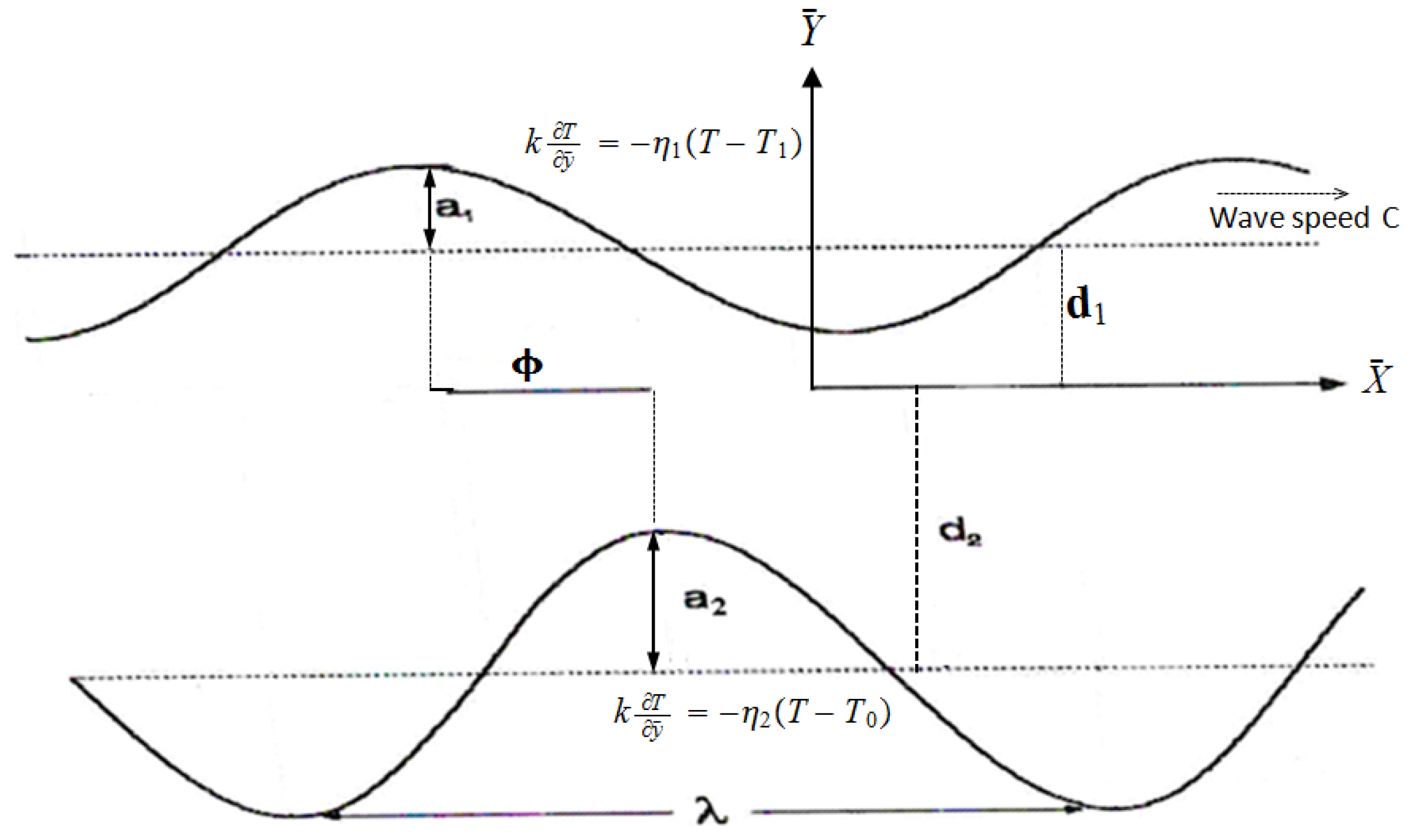
2. Formulation of Problem with Constitutive Equations

We interpret the movement of Sisko fluid through an asymmetric channel with incompressibility (see Figure 1). The fluid flow is taken along X ¯ -axis and Y ¯ axis is taken normal to the channel walls. The flow deformed is due to the following sinusoidal waves:
h ¯ 1 ( X ¯ , t ¯ ) = d 1 + a 1 cos 2 π λ ( X ¯ c t ¯ ) , upperwall , h ¯ 2 ( X ¯ , t ¯ ) = d 2 a 2 cos 2 π λ ( X ¯ c t ¯ ) + ϕ , lowerwall .
In these expressions, c denotes the wave speed, a 1 , a 2 are amplitudes of the upper and lower waves, respectively, λ is the wavelength, the width of the asymmetric channel is d 1 + d 2 , the phase difference ϕ (the range of ϕ is between 0 and π as ϕ = 0 corresponds to waves out of phase whereas ϕ = π refers to the waves that are in phase). Furthermore, a 1 , a 2 , d 1 , d 2 and ϕ fulfill the requirement given as:
a 1 2 + a 2 2 + 2 a 1 a 2 cos ϕ ( d 1 + d 2 ) 2 .
The definition of incompressibility is specified by
div V ¯ = 0 .
The laws of linear momentum and energy for the present model are
ρ d V ¯ d t ¯ = grad p ¯ + div S ¯ ,
ρ c p d T d t ¯ = k 2 T + Ø ¯ . ( grad V ¯ ) ,
where the velocity is denoted by V ¯ , density of the Sisko fluid is ρ , d / d t ¯ is material time derivative, T represents the temperature of fluid, k the thermal conductivity of the material, c p the specific heat of fluid. Body forces are not taken into account for the presented problem. Moreover, the Cauchy stress tensor is denoted by Ø ¯ = p ¯ I ¯ + S ¯ , the pressure with p ¯ , the extra stress tensor with S ¯ and 2 = 2 X ¯ 2 + 2 Y ¯ 2 (Here, the overbar corresponds to the vector quantities).
The transfer of heat with the surrounding of the walls through Newton ’s cooling law is accompanied by
k T y ¯ = η 1 ( T T 1 ) at y ¯ = h ¯ 1 ,
k T y ¯ = η 2 ( T T 0 ) at y ¯ = h ¯ 2 ,
where η 1 and η 2 , T 1 and T 0 are the heat transfer coefficients and the temperatures at the upper and the lower channel walls respectively.
For two-dimensional flow of Sisko fluid, we have the velocity V ¯ and extra stress tensor S ¯ [6,13] in the forms:
V ¯ = ( U ¯ ( X ¯ , Y ¯ , t ¯ ) , V ¯ ( X ¯ , Y ¯ , t ¯ ) , 0 ) ,
S ¯ = α + β Π ¯ n 1 A ¯ 1 ,
A ¯ 1 = L ¯ + L ¯ * , L ¯ = grad V ¯ , Π ¯ = 1 2 t r ( A ¯ 1 2 ) .
Here the fluid parameters n , α and β are defined differently for specific fluids, the second invariant of the symmetrical portion of the velocity gradient is Π ¯ and A ¯ 1 is the deformation tensor rate. It is worth mentioning that for n = 1 , β = μ , α = 0 or β = 0 , α = μ the Newtonian fluid model is obtained, and also for α = 0 the power-law model can be recovered.
If in wave-frame of reference, ( x ¯ , y ¯ ) represents the coordinates and ( u ¯ , v ¯ ) represents velocity components then we can describe
x ¯ = X ¯ c t ¯ , y ¯ = Y ¯ , u ¯ ( x ¯ , y ¯ ) = U ¯ ( X ¯ , Y ¯ , t ¯ ) c , v ¯ ( x ¯ , y ¯ ) = V ¯ ( X ¯ , Y ¯ , t ¯ ) , T ( x ¯ , y ¯ ) = T ( X ¯ , Y ¯ , t ¯ ) ,
where ( X ¯ , Y ¯ ) are the coordinates in the fixed-frame of reference. Using the above Galilean transformations and incorporating the aforementioned dimensionless variables
x = x ¯ λ , y = y ¯ d 1 , u = u ¯ c , v = v ¯ c , p = d 1 2 p ¯ c μ λ , b * = β α ( d 1 / c ) n 1 , h 1 = h ¯ 1 d 1 , h 2 = h ¯ 2 d 1 , t = c t ¯ λ , S = d 1 μ c S ¯ , θ = T T 0 T 1 T 0 ,
and the stream function ψ ( x , y ) by
u = ψ y , v = δ ψ x ,
Equation (3) is satisfied identically and Equations (4) and (5) yield
δ Re ψ y x ψ x y ψ y + p x = δ S x x x + S x y y ,
δ 3 Re ψ y x ψ x y ψ x + p y = δ 2 S x y x + δ S y y y ,
δ Re ψ y x ψ x y θ = 1 Pr δ 2 2 x 2 + 2 y 2 θ + E c δ 2 ψ x y S x x S y y + 2 ψ y 2 δ 2 2 ψ x 2 S x y ,
where the extra stress tensor components come from Equation (9). These are given by
S x x = 2 δ 1 + b * 2 ψ y 2 δ 2 2 ψ x 2 + 4 δ 2 2 ψ y x 2 2 ( n 1 ) / 2 2 ψ y x ,
S x y = 1 + b * 2 ψ y 2 δ 2 2 ψ x 2 + 4 δ 2 2 ψ y x 2 2 ( n 1 ) / 2 2 ψ y 2 δ 2 2 ψ x 2 ,
S y y = 2 δ 1 + b * 2 ψ y 2 δ 2 2 ψ x 2 + 4 δ 2 2 ψ y x 2 2 ( n 1 ) / 2 2 ψ y x .
According to the above equations, the Reynolds number Re, the dimensionless wavenumber δ , the Eckert E c and the Prandtl Pr numbers are specified by
Re = ρ c d 1 μ , δ = d 1 λ , E c = c 2 ( T 1 T 0 ) c p , Pr = μ c p k .
Now Equations (6) and (7) give
θ y + B i 1 ( θ 1 ) = 0 at y = h 1 ,
θ y + B i 2 θ = 0 at y = h 2 ,
where B i 1 = η 1 d 1 / k and B i 2 = η 2 d 1 / k are the symbols used to denote the Biot numbers.
Upon taking into consideration the assumptions of Re 0 (low Reynolds number) and δ 1 (long wavelength) [2], Equations (14) and (15) become
p x = S x y y ,
p y = 0 .
The above calculation reveals that p is independent of y. Eradicating the pressure p in Equations (23) and (24) one can obtain
2 S x y y 2 = 0 .
Furthermore, Equation (16) reduces to
2 θ y 2 + B r 2 ψ y 2 S x y = 0 ,
where the Brinkman number B r is defined by
B r = Pr E c ,
and S x y is given by
S x y = 1 + b * 2 ψ y 2 ( n 1 ) 2 ψ y 2 .
Here apparent viscosity is written as 1 + b * 2 ψ y 2 ( n 1 ) . Whenever increasing shear rate decreases the apparent viscosity, then fluid is supposed to have shear thinning effects. On the other hand, subject to the higher shear rate, if the apparent viscosity increases, then fluid is called shear thickening fluid. Therefore, Equation (28) describes that when n < 1 , fluid exhibits shear thinning effects whereas when n > 1 , it shows shear thickening effects. But when n = 1 one can obtain the case of Newtonian fluid.
In the fixed-frame, the instant volume flow rate is represented as
Q = h ¯ 2 ( X ¯ , t ¯ ) h ¯ 1 ( X ¯ , t ¯ ) U ¯ ( X ¯ , Y ¯ , t ¯ ) d Y ¯ .
The volume flow rate q in moving frame is
q = h ¯ 2 ( x ¯ ) h ¯ 1 ( x ¯ ) u ¯ ( x ¯ , y ¯ ) d y ¯ .
From Equations (11), (29) and (30) we can write
Q = q + c h ¯ 1 ( x ¯ ) c h ¯ 2 ( x ¯ ) .
Over a period τ , the time-mean flow denoted by Q ¯ is calculated as
Q ¯ = 1 τ 0 τ Q d t ¯ .
Merging Equations (31) and (32) and integrating the subsequent expression, one can get
Q ¯ = q + c d 1 + c d 2 .
Classifying the dimensionless time-mean flows as F and Θ in the wave and laboratory frames respectively by
F = q c d 1 , Θ = Q ¯ c d 1 ,
Equation (33) becomes
Θ = F + 1 + d ,
with
F = h 2 ( x ) h 1 ( x ) ψ y d y = ψ ( h 1 ( x ) ) ψ ( h 2 ( x ) ) .
The dimensionless forms of h i ( i = 1 , 2 ) are
h 1 ( x ) = 1 + a cos ( 2 π x ) , h 2 ( x ) = d b cos ( 2 π x + ϕ ) ,
where a = a 1 / d 1 , b = a 2 / d 1 , d = d 2 / d 1 and ϕ obey the following relationship
a 2 + b 2 + 2 a b cos ϕ ( 1 + d ) 2 .
In moving frame, the dimensionless stream function has the following conditions at the walls:
ψ = F 2 , ψ y = 1 , at y = h 1 ( x ) ,
ψ = F 2 , ψ y = 1 , at y = h 2 ( x ) .

3. Systematic Solution Process

The resultant Equation (25) is an exceptionally non-linear. The exact solution in closed form appears unlikely for arbitrary values of parameters included in this equation. To solve the highly nonlinear differential equations, we have used the regular perturbation method based on a small parameter as exact solution is not possible. This method is useful for finding an approximate solution to the problem, by starting from the exact solution of a related and simpler problem. This method is more effective as it gives the solution in form of convergent series. Priority is therefore based on the small parameter b * which will give series solutions. That is why we are going to expand ψ , θ , S x y , p and F as:
ψ = ψ 0 + ( b * ) ψ 1 + . . . , θ = θ 0 + ( b * ) θ 1 + . . . , S x y = S 0 x y + ( b * ) S 1 x y + . . . , p = p 0 + ( b * ) p 1 + . . . , F = F 0 + ( b * ) F 1 + . . . .
Replacement of equations described above into Equations (21)–(26), (28), (31), (39), (40) and then accumulating the like power terms of b * , we get the following systems of equations:

3.1. Zeroth Order System

4 ψ 0 y 4 = 0 ,
2 θ 0 y 2 + B r 2 ψ 0 y 2 S 0 x y = 0 ,
d p 0 d x = 3 ψ 0 y 3 ,
ψ 0 = F 0 2 , ψ 0 y = 1 , θ 0 y + B i 1 ( θ 0 1 ) = 0 , at y = h 1 ( x ) ,
ψ 0 = F 0 2 , ψ 0 y = 1 , θ 0 y + B i 2 θ 0 = 0 , at y = h 2 ( x ) .

3.2. First Order System

2 y 2 2 ψ 0 y 2 n + 2 ψ 1 y 2 = 0 ,
2 θ 1 y 2 + B r 2 2 ψ 0 y 2 2 ψ 1 y 2 + 2 ψ 0 y 2 n + 1 = 0 ,
d p 1 d x = y 2 ψ 0 y 2 n + 2 ψ 1 y 2 ,
ψ 1 = F 1 2 , ψ 1 y = 0 , θ 1 y + B i 1 θ 1 = 0 , at y = h 1 ( x ) ,
ψ 1 = F 1 2 , ψ 1 y = 0 , θ 1 y + B i 2 θ 1 = 0 , at y = h 2 ( x ) .
In the subsequent two subsections, we will evolve the solutions of above systems.

3.3. Solution at Zeroth Order

The solutions to the Equations (42) and (43) according to the constraints mentioned in Equations (45) and (46) are
ψ 0 = R 1 y 3 + R 2 y 2 + R 3 y + R 4 ,
θ 0 = A 1 y 4 + A 2 y 3 + A 3 y 2 + A 4 y + A 5 ,
where the quantities involved in above equations are given in Appendix A.
The longitudinal velocity and pressure gradient are given by
u 0 = 3 R 1 y 2 + 2 R 2 y + R 3 ,
d p 0 d x = 6 R 1 .
The dimensionless form of pressure rise per wavelength is denoted by ( Δ P λ 0 ) and obtained by
Δ P λ 0 = 0 1 d p 0 d x d x .
We noticed that the solutions presented at this order refer to the solutions of Newtonian fluid flow.

3.4. Solution at First Order

Using Equation (52) into Equations (47)–(49), resolving the corresponding equations and implementing the relevant boundary conditions, the first-order solutions for ψ 1 , u 1 , d p 1 / d x and θ 1 are obtained in the forms given below.
ψ 1 = 1 6 B 11 ( h 1 h 2 ) 3 [ 3 F 1 B 11 B 16 6 h 2 y 2 + 4 y 3 + 3 h 1 ( h 2 2 4 h 2 y + 2 y 2 ) + 2 n + 1 { 2 R 2 2 B 17 y 3 3 h 2 2 R 1 y 2 ( B 19 3 n R 1 B 13 y ) 3 h 2 R 2 y 2 ( B 20 B 21 y ) + h 2 3 ( 3 R 1 R 2 y ( B 22 2 ( R 2 + 3 R 1 y ) n ) + R 2 2 ( B 12 ( R 2 + 3 R 1 y ) n ) 9 R 1 2 y 2 ( B 23 + ( R 2 + 3 R 1 y ) n ) ) + h 1 3 ( B 24 3 R 1 R 2 y ( B 25 2 ( R 2 + 3 R 1 y ) n ) + 9 R 1 2 y 2 ( B 26 + ( R 2 + 3 R 1 y ) n ) + R 2 2 ( B 13 + ( R 2 + 3 R 1 y ) n ) 3 h 2 R 1 ( B 27 y + n ( B 28 + B 29 y ) ) ) 3 h 1 2 ( B 30 h 2 2 R 1 B 17 ( B 31 + B 32 y ) + R 1 y 2 ( B 33 + B 34 y ) + h 2 ( 3 R 1 2 y 2 ( B 35 3 ( R 2 + 3 R 1 y ) n ) + R 2 2 ( B 13 + ( R 2 + 3 R 1 y ) n ) + R 1 R 2 y ( B 36 + 6 ( R 2 + 3 R 1 y ) n ) ) ) + 3 h 1 ( R 2 y 2 ( B 20 + B 37 y ) + h 2 B 17 y ( B 38 + B 39 y + B 40 y 2 ) + h 2 3 R 1 ( B 27 y + n ( B 41 + B 42 y ) ) + h 2 2 ( 3 R 1 2 y 2 ( B 43 3 ( R 2 + 3 R 1 y ) n ) + R 2 2 ( B 12 + ( R 2 + 3 R 1 y ) n ) + R 1 R 2 y ( B 44 + 6 ( R 2 + 3 R 1 y ) n ) ) ) } ] ,
u 1 = M 1 + M 2 y + M 3 y 2 + M 4 ( R 2 + 3 R 1 y ) n + 1 ,
d p 1 d x = 2 ( h 1 h 2 ) 3 B 11 [ 6 F 1 B 11 + 2 n { B 14 + 2 R 2 2 ( B 12 B 13 ) + 3 h 2 R 1 R 2 ( ( n + 2 ) B 12 + ( n 2 ) B 13 ) + 3 h 1 R 1 ( B 15 R 2 ( ( n 2 ) B 12 + ( n + 2 ) B 13 ) ) } ] ,
where the quantities described in the above calculations are displayed in Appendix A. Furthermore,
θ 1 = L 1 ( R 2 + 3 R 1 y ) n + 3 + L 2 y 4 + L 3 y 3 + L 4 y 2 + L 5 y + L 6 ,
in which the values ( L 1 L 6 ) are being conveniently obtained by algebraic calculations.
Over a period 2 π , the pressure rise per wavelength is denoted by ( Δ P λ 1 ) and calculated as follows:
Δ P λ 1 = 0 2 π d p 1 d x d x .
The perturbation expressions of ψ , θ , Δ P λ and d p / d x upto O ( b * ) 1 are
ψ = ψ 0 + ( b * ) ψ 1 . θ = θ 0 + ( b * ) θ 1 . d p d x = d p 0 d x + ( b * ) d p 1 d x . Δ P λ = Δ P λ 0 + ( b * ) Δ P λ 1 .

4. Results and Discussion

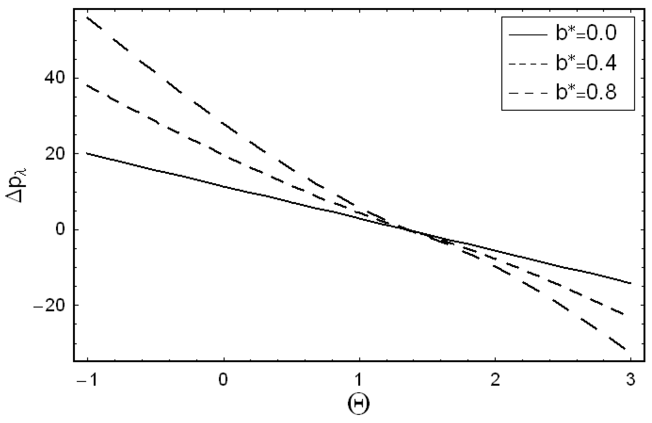
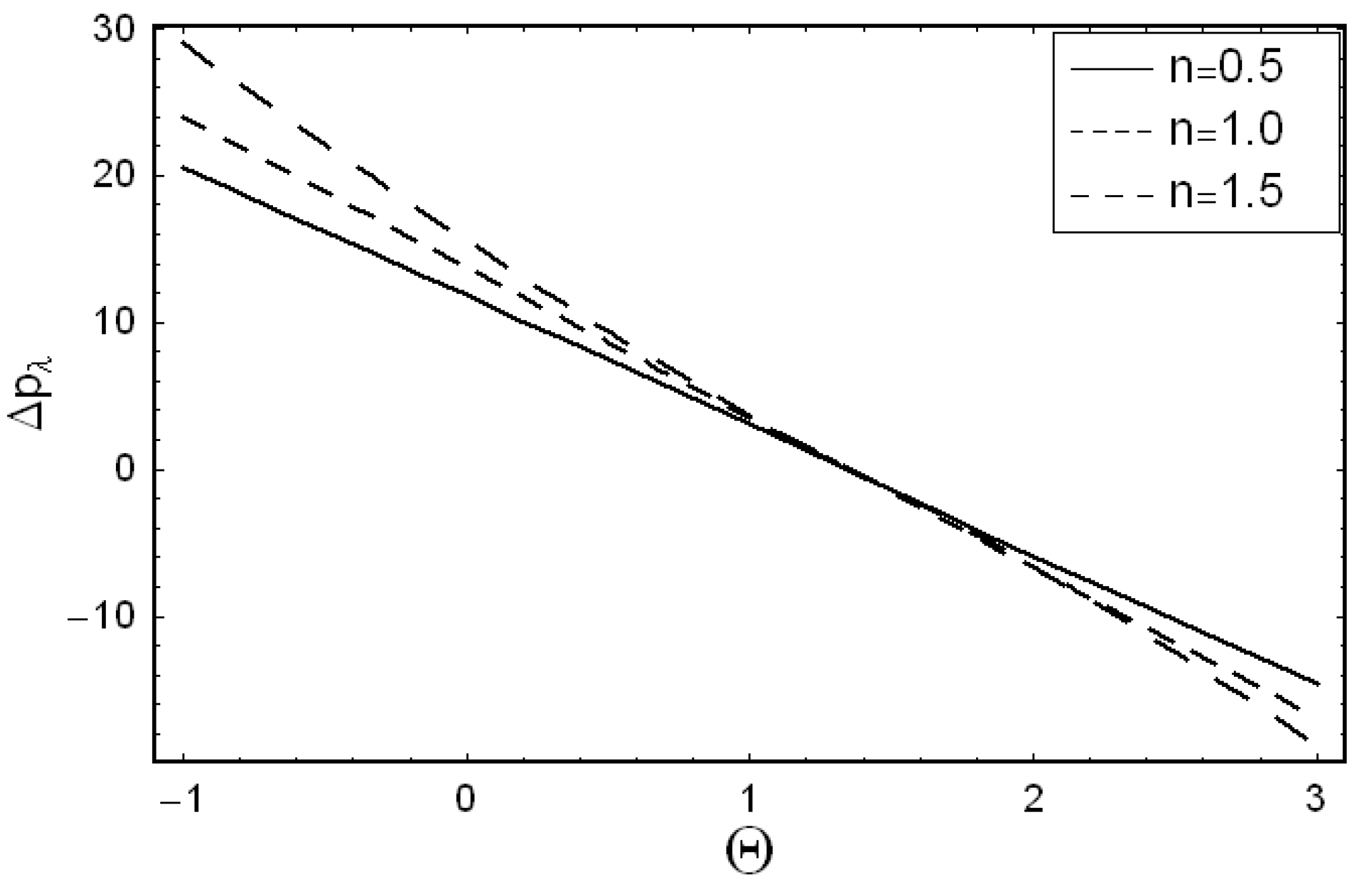
4.1. Pumping Characteristics

In this section the perturbed results of the Sisko fluid model are illustrated in Figure 2, Figure 3, Figure 4, Figure 5, Figure 6 and Figure 7. The variability of pressure gradient ( d p d x ) for particular values of the sundry parameters are seen in the Figure 2, Figure 3 and Figure 4. The alteration of the pressure gradient d p d x for non-identical values of the Sisko fluid parameter b * is sketched in Figure 2. The material parameter b * for Sisko fluid shows the ratio of a power-law component to a viscous part if n 1 . When n 1 , b * = 0 denotes a viscous fluid. Therefore, Figure 2 predicts that d p d x across the narrow part of the channel is constructive and therefore prevents the flow. But in the wider part of the channel, d p d x is negative which facilitates the passage of fluid. For such a case the peristaltic pumping is more dominant and movement is in the peristaltic direction. Figure 3 reflects the influence of various values of the phase difference ϕ on d p d x . The Figure 3 clearly shows that the longitudinal distribution of d p d x dissipates as the phase difference ϕ rises. In Figure 4 the axial distribution of d p d x is depicted for three non-identical values of n. The fascinating phenomena (found in Figure 4) is that, generally, the difference of d p d x for the shear-thickening fluid ( n > 1 ) is much higher than that for the shear-thinning fluid ( n < 1 ) although these phenomena described above are same in a qualitative sense for the Newtonian fluid ( n = 1 ) , a shear-thickening fluid and a shear-thinning fluid. The difference between all these cases is easily identified when total pressure rise over a wavelength is considered. Notice that determining pressure rise requires the integration of d p d x . The integral which emerges is non-analytically solvable. Consequently, the associated integral is determined numerically. Figure 5, Figure 6 and Figure 7 illustrate the relation between pressure rise per wavelength ( Δ p λ ) versus flow rate ( Θ ) for several values of b * , ϕ and n, respectively. It is perceived that Δ p λ increases with an increase in b * and n (Figure 5 and Figure 7) and decreases with increasing ϕ (Figure 6). Effects of various Sisko fluid parameter and phase differences are displayed in the Figure 5 and Figure 6 only for a shear-thickening fluid ( n = 1.5 ) . From Figure 7, for a Newtonian fluid ( n = 1 ), a linear relationship is observed between Δ p λ and Θ . Physically, the positive values of flow rate assists the peristaltic pumping whereas the negative values of flow rate opposes the peristaltic pumping which is called retrograde pumping. For a shear-thickening fluid ( n > 1 ) , quite higher d p d x is required than for a shear-thinning fluid. ( n < 1 ) . That is indeed in-between for the Newtonian fluid ( n = 1 ) .

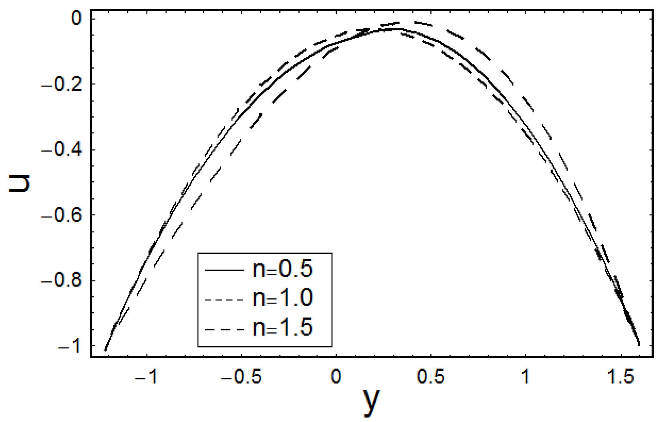
4.2. Velocity Profile

As the peristaltic flows in channel are considered as Poiseuille flow, therefore, the maximum velocity is at the center of the channel. This subsection is dealt to observe this phenomenon. Figure 8a,b display the influence of b * on the fluid velocity u for two different values of the power-law exponent n = 0.5 and n = 1.5 , respectively. It is perceived that increasing b * strengthens the power-law effect of Sisko fluid under investigation. In the case of n = 0.5 , increasing b * originates the thin boundary layers. In contrast, when n = 1.5 , increasing b * is a source of thicker boundary layers. Figure 9 shows the velocity profile with three different power values n. Here, for better understanding of fluid’s rheology, we explore the shear-thickening ( n = 1.5 ) and shear-thinning ( n = 0.5 ) fluids and then make a comparison with Newtonian fluid ( n = 1 ). Obviously, for a shear-thickening fluid ( n = 1.5 ) , no sharp boundary layers are emerged along the surface of the wall. Conversely, for a shear-thinning fluid ( n = 0.5 ) , two thin boundary layers can be observed just next to both walls. Behavior in Newtonian fluid ( n = 1 ) resides between the two cases.

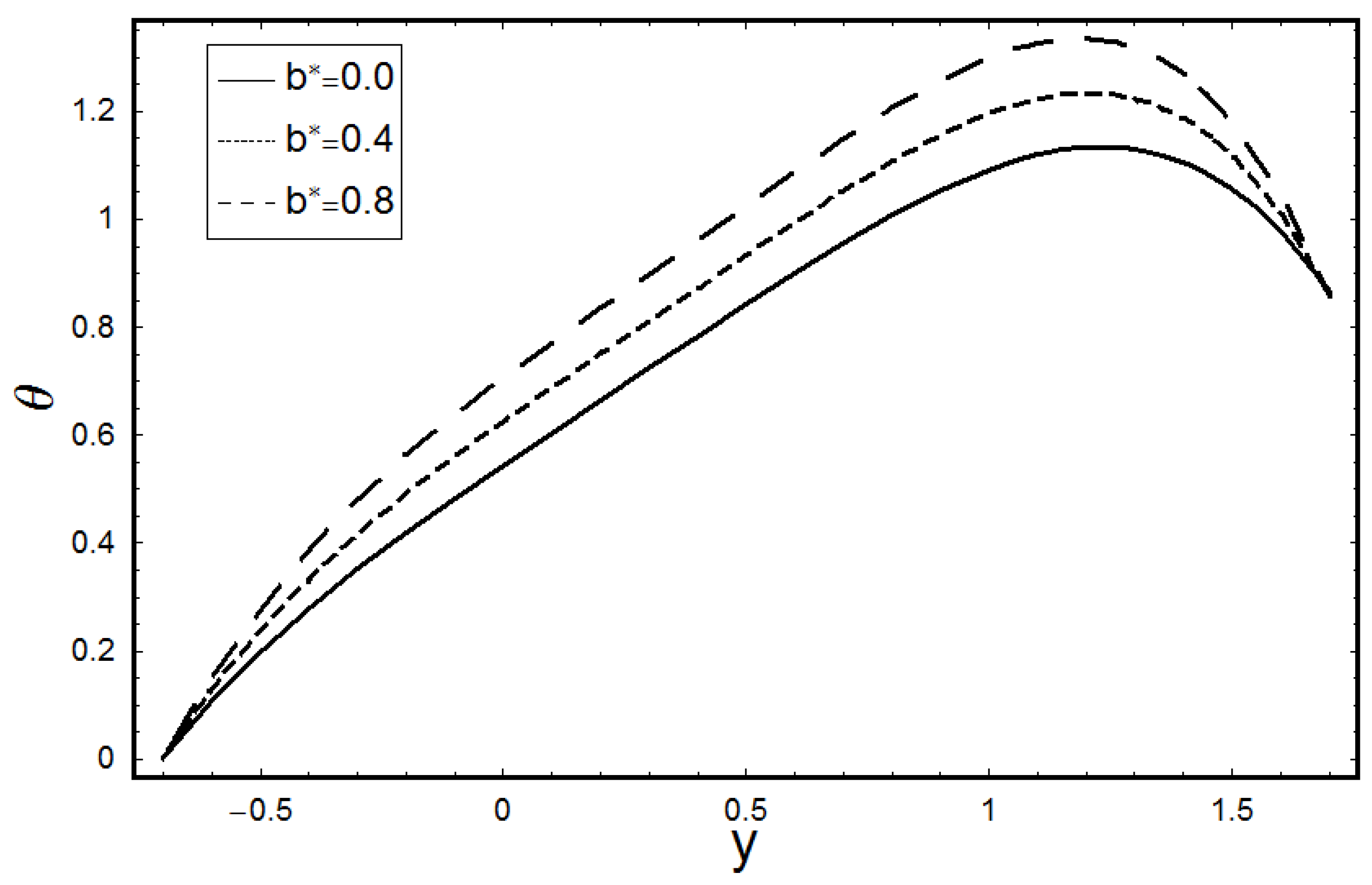
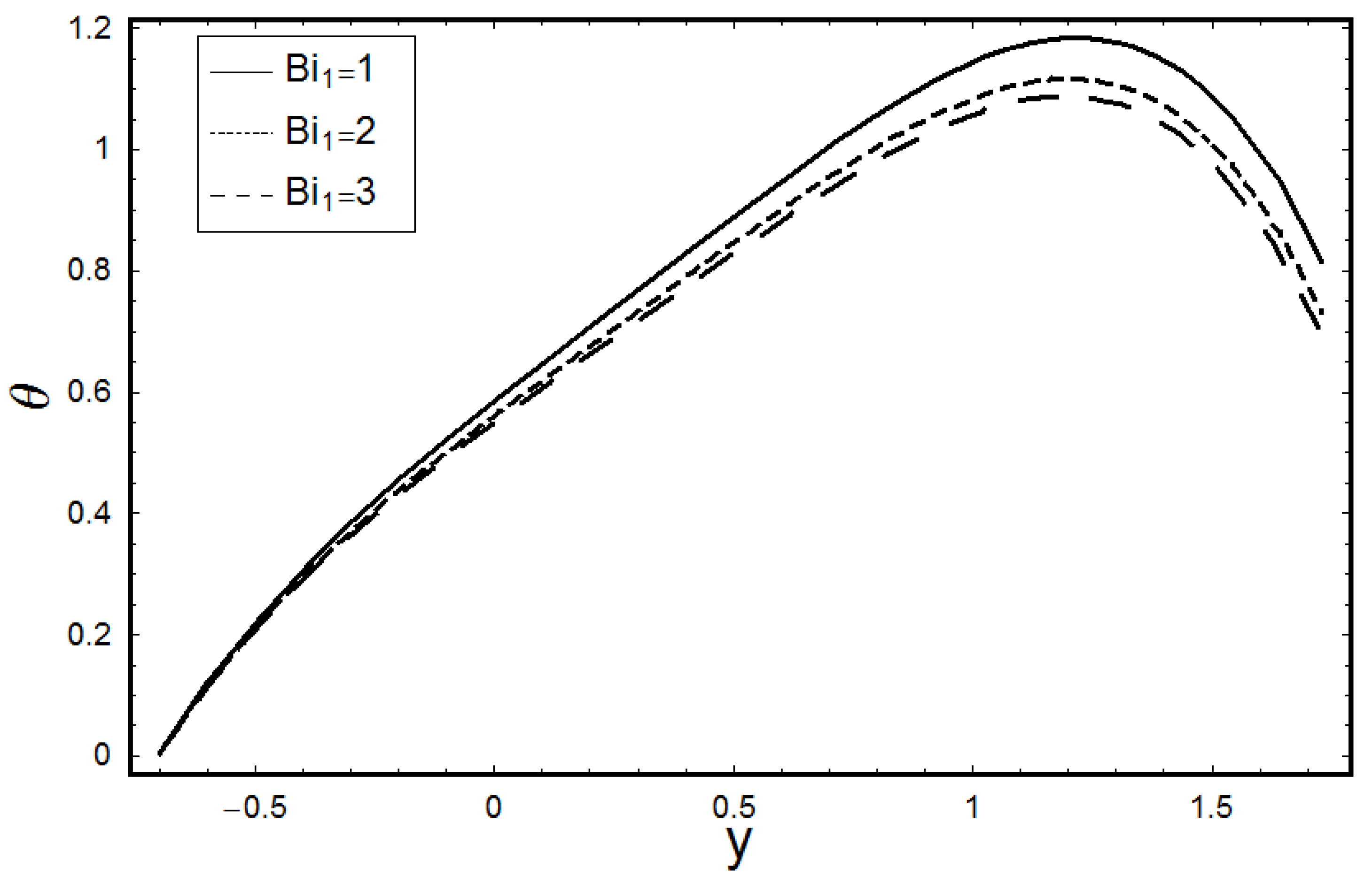
4.3. Heat Transfer Profile
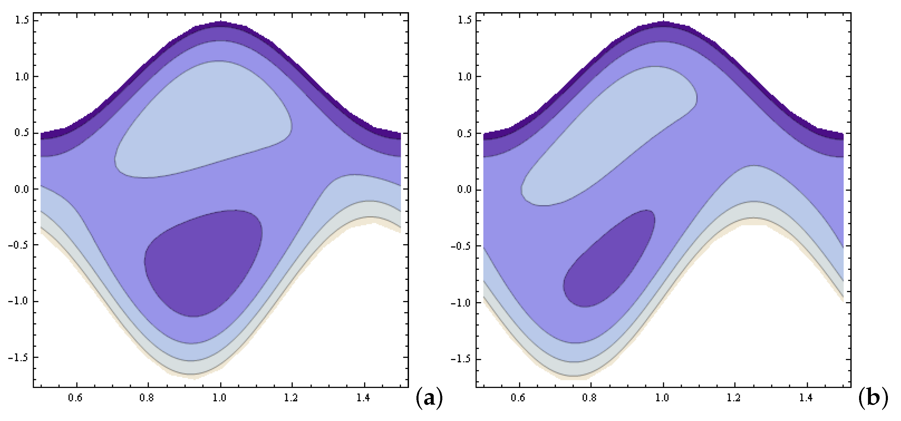
The results of various evolving parameters on the temperature profile θ are addressed here. Figure 10 and Figure 11 indicate the rise in fluid temperature attributed to convective conditions (for shear-thickening fluid only). It should be noted that the fluid temperature, in general, increases with an increase in the value of material parameter b * and the Brinkman number B r . Figure 12 portrays the influence of Biot number B i 1 on temperature profile θ (for shear-thickening fluid n = 1.5 ). This figure demonstrates that the temperature profile θ for the Biot number B i 1 reduces at the upper wall of the channel by rising the Biot number B i 1 while it does not show any effect near the lower channel wall. Figure 13 illustrates the effects of Biot number B i 2 on temperature profile θ (for shear-thickening fluid n = 1.5 ). It is observed that the temperature θ increases near the lower wall by increasing the Biot number B i 2 . The values of Biot numbers are taken to be larger than 1 which shows the nonuniform temperature fields within the fluid. It also shows that convection is much faster than conduction. So the chosen parameters are realistic from practical point of view because of their application in biomechanics, heat exchangers, gas turbines etc.. The effect of different power values n on the temperature can also be clearly observed from Figure 14. This figure indicates that the temperature intensifies for n = 1.5 (shear-thickening fluid) then that of a shear-thinning fluid ( n = 0.5 ) . Moreover for ( n = 1 ) it lies above these two.

4.4. Trapping

Usually, in the wave/moving frame, the shape of streamlines is related to the boundary wall movement. However, some of the streamlines split and surround a bolus under certain conditions and this bolus moves entirely with the wave. This is a well-known phenomenon called trapping. Figure 15 shows the streamlines for n = 0.5 (panels (a), (b)), n = 1 (panels (c), (d)) and n = 1.5 (panels (e), (f)) with two values of phase difference, i.e., ϕ = 0 (left panels) and ϕ = π / 2 (right panels). Near the channel walls, streamlines strictly follow the waves on walls and these waves are generated due to relative motion of the distensible channel walls. Further, a bolus is formed in the central region. When we compare the flow fields which are obtained from choosing different values of n, we depict that the bolus alteration is slower for shear-thinning fluid (i.e., panels (a) and (b)) than that for a shear-thickening fluid (i.e., panels (e) and (f)). Furthermore, Newtonian fluid case lies between these two.

5. Major Outcomes

This article is written to investigate the motion of Sisko fluid under the effects of convective conditions at the walls if asymmetric channel. Comparison is presented between shear-thickening, Newtonian and shear-thinning fluids by choosing different values of material parameters. Peristaltic flow characteristics such as trapping and pumping are reported from the presented perturbed results. Pressure rise per wavelength increases with an increase in Sisko fluid parameter which assist the fluid flow. The slower alteration in the size of the trapping bolus is observes for shear-thinning fluid than that for a shear-thickening fluid. The thermal analysis indicates that the implementation of a rise in a non-Newtonian parameter, the Biot numbers and Brinkman number increases the thermal stability of the liquid. To the best of our knowledge, such observations have never been reported for the peristaltic flow of Sisko fluid.

Author Contributions

Conceptualization, H.Y.; formal analysis, A.A.A.; investigation, N.I.; methodology, H.Y.; software, N.I. and H.Y.; validation, B.K.K. and A.A.A.; writing-original draft preparation, H.Y. and N.I.; writing-review and editing, N.I., B.K.K. and A.A.A.; visualization, N.I. and H.Y.; supervision, H.Y. All authors have read and agreed to the published version of the manuscript.

Funding

This research has been funded by Scientific Research Deanship at University of Ha’il, Saudi Arabia through project number RG-191323.

Conflicts of Interest

The authors declare no conflict of interest.

Appendix A

Here we provide the quantities appearing in the flow analysis:
R 1 = 2 ( F 0 + h 1 h 2 ) ( h 1 h 2 ) 3 , R 2 = 3 ( F 0 + h 1 h 2 ) ( h 1 + h 2 ) ( h 1 h 2 ) 3 , R 3 = h 1 3 6 F 0 h 1 h 2 3 h 1 2 h 2 + 3 h 1 h 2 2 + h 2 3 ( h 1 h 2 ) 3 , R 4 = ( h 1 + h 2 ) ( 2 h 1 h 2 ( h 1 + h 2 ) + F 0 ( h 1 2 4 h 1 h 2 + h 2 2 ) ) 2 ( h 1 h 2 ) 3 , B 1 = B i 2 + B i 1 ( 1 + B i 2 ( h 1 h 2 ) ) , B 2 = 3 h 1 2 R 1 2 + 3 h 1 R 1 R 2 + R 2 2 , B 3 = 3 h 2 2 R 1 2 + 3 h 2 R 1 R 2 + R 2 2 , B 4 = 3 ( h 1 4 h 2 4 ) R 1 2 + 4 ( h 1 3 h 2 3 ) R 1 R 2 + 2 ( h 1 2 h 2 2 ) R 2 2 , B 5 = 1 + B i 2 h 2 , B 6 = 4 h 1 B 2 B 5 , B 7 = 9 h 2 2 R 1 2 + 8 h 2 R 1 R 2 + 2 R 2 2 , B 8 = B 3 + h 2 R 1 R 2 + R 2 2 , B 9 = 3 ( h 1 3 4 h 2 3 ) R 1 2 4 ( h 1 2 3 h 2 2 ) R 1 R 2 2 ( h 1 2 h 2 2 ) R 2 2 , B 10 = 3 ( h 1 3 + h 2 3 ) R 1 2 + 4 ( h 1 2 + h 2 2 ) R 1 R 2 + 2 ( h 1 + h 2 ) R 2 2 , A 1 = 3 B r R 1 2 , A 2 = 4 B r R 1 R 2 , A 3 = 2 B r R 2 2 , A 4 = 1 B 1 [ 4 B i 2 B r h 1 B 2 + B i 1 { 4 B r h 2 B 3 + B i 2 ( 1 + B r B 4 ) } ] , A 5 = 1 B 1 [ B r { B 6 + h 2 ( B 7 + B 5 B 8 ) } + B i 1 { 1 + B r h 1 B 9 + B i 2 h 2 ( 1 + B r h 1 B 10 ) } ] , B 11 = ( 2 + 3 n + n 2 ) R 1 2 , B 12 = ( 3 h 1 R 1 + R 2 ) n , B 13 = ( 3 h 2 R 1 + R 2 ) n , B 14 = 9 n R 1 2 ( h 1 2 B 12 + h 2 2 B 13 ) , B 15 = ( n 2 ) B 12 + ( n + 2 ) B 13 , B 16 = h 1 3 3 h 1 2 h 2 + h 2 2 , B 17 = B 12 B 13 , B 18 = B 12 + B 13 , B 19 = R 2 ( 4 B 17 + n ( B 12 + B 18 ) ) , B 20 = R 2 B 17 , B 21 = R 1 ( B 12 + B 17 + n B 18 ) , B 22 = ( n + 2 ) B 12 , B 23 = ( n 1 ) B 13 , B 24 = 9 h 2 2 R 1 2 ( B 17 + n B 18 ) , B 25 = ( n + 2 ) B 13 , B 26 = ( n 1 ) B 12 , B 27 = 6 R 1 B 17 , B 28 = R 2 B 13 , B 29 = 6 R 1 B 18 , B 30 = 3 h 2 2 R 1 2 ( B 17 + n B 18 ) , B 31 = ( n 4 ) R 2 , B 32 = 3 ( n + 2 ) R 1 , B 33 = R 2 ( 4 B 17 + n ( B 18 + B 13 ) ) , B 34 = 3 n R 1 B 12 , B 35 = ( n 1 ) B 12 + ( 2 n + 4 ) B 13 , B 36 = ( 2 n 8 ) B 12 + ( n + 2 ) B 13 , B 37 = R 1 ( 2 B 17 + n B 18 ) , B 38 = 2 R 2 2 , B 39 = ( n 4 ) R 1 R 2 , B 40 = 3 ( n + 2 ) R 1 2 , B 41 = R 2 B 12 , B 42 = 3 R 1 ( B 12 + 2 B 13 ) , B 43 = ( 2 n + 4 ) B 12 + ( n 1 ) B 13 , B 44 = ( n + 2 ) B 12 + ( 2 n 8 ) B 13 , M 1 = 1 B 11 ( h 1 h 2 ) 3 [ 6 B 11 F 1 h 1 h 2 + 2 n B 17 h 1 h 2 ( B 38 + B 32 h 1 h 2 R 1 ) 2 n R 1 { B 27 h 1 h 2 ( h 1 2 + h 2 2 ) + n B 29 h 1 3 h 2 n B 42 h 1 h 2 3 + ( B 25 h 1 3 h 2 ( B 36 h 1 2 + h 2 ( B 44 h 1 + B 22 h 2 ) ) ) R 2 } ] , M 2 = 2 B 11 ( h 1 h 2 ) 3 [ 3 B 11 F 1 ( h 1 h 2 ) + 2 n { B 17 B 39 h 1 h 2 + R 1 ( B 33 h 1 2 + 3 B 26 h 1 3 R 1 h 2 ( 3 B 35 h 1 2 R 1 + h 2 ( B 19 + 3 ( B 43 h 1 + B 23 h 2 ) R 1 ) ) ) B 20 ( h 1 + h 2 ) R 2 } ] , M 3 = 1 B 11 ( h 1 h 2 ) 3 [ 6 B 11 F 1 + 2 n { 3 B 17 B 40 h 1 h 2 3 B 34 h 1 2 R 1 + 9 n B 13 h 2 2 R 1 2 3 B 37 h 1 R 2 + 3 B 21 h 2 R 2 + 2 B 17 R 2 2 } ] , M 4 = 2 n ( n + 2 ) R 1 B 11 .

References

  1. Latham, T.W. Fluid Motion in a Peristaltic Pump. Master’s Thesis, MIT, Cambridge, MA, USA, 1966. [Google Scholar]
  2. Shapiro, A.H.; Jaffrin, M.Y.; Weinberg, S.L. Peristaltic pumping with long wavelengths at low Reynolds number. J. Fluid Mech. 1969, 37, 799–825. [Google Scholar] [CrossRef]
  3. Jaffrin, M.Y.; Shapiro, A.H. Peristaltic pumping. Ann. Rev. Fluid Mech. 1971, 3, 13–37. [Google Scholar] [CrossRef]
  4. Rath, H.J. Peristaltic flow through a lobe-shaped tube. Int. J. Mech. Sci. 1982, 24, 359–367. [Google Scholar] [CrossRef]
  5. Mekheimer, K.S.; Abdellateef, A.I. Peristaltic transport through eccentric cylinders: Mathematical model. Appl. Bio. Biomech. 2013, 10, 19–27. [Google Scholar] [CrossRef]
  6. Khan, A.S.; Nie, Y.; Shah, Z. Impact of thermal radiation on magnetohydrodynamic unsteady thin film flow of Sisko fluid over a stretching surface. Processes 2019, 7, 369. [Google Scholar] [CrossRef] [Green Version]
  7. Ramesh, K.; Tripathi, D.; Bhatti, M.M.; Khalique, C.M. Electro-osmotic flow of hydromagnetic dusty viscoelastic fluids in a microchannel propagated by peristalsis. J. Mol. Liq. 2020, 314, 113568. [Google Scholar] [CrossRef]
  8. Tariq, H.; Khan, A.A.; Zaman, A. Theoretical analysis of peristaltic viscous fluid with inhomogeneous dust particles. Arab. J. Sci. Eng. 2020. [Google Scholar] [CrossRef]
  9. Bhandari, D.S.; Tripathi, D.; Narla, V.K. Pumping flow model for couple stress fluids with a propagative membrane contraction. Int. J. Mech. Sci. 2020. [CrossRef]
  10. Abd-Alla, A.M.; Abo-Dahab, S.M. Magnetic field and rotation effects on peristaltic transport of a Jeffrey fluid in an asymmetric channel. J. Magn. Magn. Mat. 2015, 374, 680–689. [Google Scholar] [CrossRef]
  11. Lachiheb, M. Effect of coupled radial and axial variability of viscosity on the peristaltic transport of Newtonian fluid. Appl. Math. Comput. 2014, 244, 761–771. [Google Scholar]
  12. Javed, M. A mathematical framework for peristaltic mechanism of non-Newtonian fluid in an elastic heated channel with Hall effect. Multidis. Model. Mat. Struct. 2020. [Google Scholar] [CrossRef]
  13. Ahmed, B.; Hayat, T.; Alsaedi, A.; Abbasi, F.M. Joule heating in mixed convective peristalsis of Sisko nanomaterial. J. Therm. Anal. Calorim. 2020. [Google Scholar] [CrossRef]
  14. Nadeem, S.; Abbas, N.; Malik, M.Y. Heat transport in CNTs based nanomaterial flow of non-Newtonian fluid having electro magnetize plate. Alex. Eng. J. 2020. [Google Scholar] [CrossRef]
  15. Abbasi, F.M.; Gul, M.; Shehzad, S.A. Effectiveness of temperature-dependent properties of Au, Ag, Fe3O4, Cu nanoparticles in peristalsis of nanofluids. Int. Commun. Heat Mass Transf. 2020, 116, 104651. [Google Scholar] [CrossRef]
  16. Nisar, Z.; Hayat, T.; Alsaedi, A.; Ahmad, B. Significance of activation energy in radiative peristaltic transport of Eyring-Powell nanofluid. Int. Commun. Heat Mass Transf. 2020, 116, 104655. [Google Scholar] [CrossRef]
  17. Khan, A.S.; Nie, Y.; Shah, Z. Impact of thermal radiation and heat source/sink on MHD time-dependent thin-film flow of Oldroyed-B, Maxwell, and Jeffery fluids over a stretching surface. Processes 2019, 7, 191. [Google Scholar] [CrossRef] [Green Version]
  18. Reddy, M.G. Heat and mass transfer on magnetohydrodynamic peristaltic flow in a porous medium with partial slip. Alex. Eng. J. 2016, 55, 1225–1234. [Google Scholar] [CrossRef]
  19. Hayat, T.; Yasmin, H. Maryem Al-Yami, Soret and Dufour effects in peristaltic transport of physiological fluids with chemical reaction: A mathematical analysis. Comput. Fluids 2014, 89, 242–253. [Google Scholar] [CrossRef]
  20. Bhatti, M.M.; Ellahi, R.; Zeeshan, A.; Marin, M.; Ijaz, N. Numerical study of heat transfer and Hall current impact on peristaltic propulsion of particle-fluid suspension with compliant wall properties. Mod. Phys. Lett. B 2019, 33, 1950439. [Google Scholar] [CrossRef]
  21. Riaz, A.; Ellahi, R.; Sait, S.M. Role of hybrid nanoparticles in thermal performance of peristaltic flow of Eyring-Powell fluid model. J. Them. Anal. Calorim. 2020. [Google Scholar] [CrossRef]
  22. Ahmed, R.; Ali, N.; Ullah Khan, S.; Tlili, I. Numerical simulations for mixed convective hydromagnetic peristaltic flow in a curved channel with joule heating features. AIP Adv. 2020, 10, 075303. [Google Scholar] [CrossRef]
  23. Abbas, M.A.; Bhatti, M.M.; Rashidi, M.M. Heat transfer on magnetohydrodynamic stagnation point flow through a porous shrinking/stretching sheet: A numerical study. Therm. Sci. 2020, 24, 1335–1344. [Google Scholar] [CrossRef]
  24. Riaz, A.; Bhatti, M.M.; Ellahi, R.; Zeeshan, A.; Sait, S.M. Mathematical analysis on an asymmetrical wavy motion of blood under the influence entropy generation with convective boundary conditions. Symmetry 2020, 12, 102. [Google Scholar] [CrossRef] [Green Version]
  25. Hina, S.; Hayat, T.; Asghar, S.; Hendi, A.A. Influence of compliant walls on peristaltic motion with heat/mass transfer and chemical reaction. Int. J. Heat Mass Transf. 2012, 55, 3386–3394. [Google Scholar] [CrossRef]
  26. Hayat, T.; Yasmin, H.; Alsaedi, A. Peristaltic flow of couple stress fluid in an asymmetric channel with convective conditions. Heat Transf. Res. 2016, 47, 327–342. [Google Scholar] [CrossRef]
  27. Yasmin, H.; Farooq, S.; Awais, M.; Alsaedi, A.; Hayat, T. Significance of heat and mass process in peristalsis of a rheological material. Heat Transf. Res. 2019, 50, 1561–1580. [Google Scholar] [CrossRef]
  28. Hayat, T.; Bibi, A.; Yasmin, H.; Alsaadi, F.E. Magnetic field and thermal radiation effects in peristaltic flow with heat and mass convection. J. Therm. Sci. Eng. Appl. 2018, 10, 051018. [Google Scholar] [CrossRef]
  29. Hussain, Q.; Hayat, T.; Asghar, S.; Alsaedi, A. Heat transfer in a porous saturated wavy channel with asymmetric convective boundary conditions. J. Cent. South Univ. 2015, 22, 392–401. [Google Scholar] [CrossRef]
  30. Danook, S.H.; Jasim, Q.K.; Hussein, A.M. Nanofluid convective heat transfer enhancement elliptical tube inside circular tube under turbulent flow. Math. Comput. Appl. 2018, 23, 78–87. [Google Scholar]
  31. Mkhatshwa, M.; Motsa, S.; Sibanda, P. Overlapping multi-domain spectral method for conjugate problems of conduction and MHD Free convection flow of nanofluids over flat plates. Math. Comput. Appl. 2019, 24, 75–102. [Google Scholar]
Figure 1. Geometry of the problem.
Mca 25 00052 g001
Figure 2. Variation in d p / d x for b * with a = 1.0 , b = 0.7 , d = 1.2 , n = 1.5 , ϕ = π / 2 and Θ = 1 .
Mca 25 00052 g002
Figure 3. Variation in d p / d x for ϕ with a = 1.0 , b = 0.7 , d = 1.2 , n = 1.5 , b * = 0.2 and Θ = 1 .
Mca 25 00052 g003
Figure 4. Variation in d p / d x for n with a = 1.0 , b = 0.7 , d = 1.2 , b * = 0.2 , ϕ = π / 2 and Θ = 1 .
Mca 25 00052 g004
Figure 5. Variation in Δ p λ versus Θ for b * with a = 1.0 , b = 0.7 , d = 1.2 , n = 1.5 and ϕ = π / 4 .
Mca 25 00052 g005
Figure 6. Variation in Δ p λ versus Θ for ϕ with a = 1.0 , b = 0.7 , d = 1.2 , n = 1.5 and b * = 0.2 .
Mca 25 00052 g006
Figure 7. Variation in Δ p λ versus Θ for n with a = 1.0 , b = 0.7 , d = 1.2 , b * = 0.2 and ϕ = π / 4 .
Mca 25 00052 g007
Figure 8. (a) Plot of u for b * with a = 0.6 , b = 0.3 , d = 1.0 , ϕ = π / 4 , Θ = 1 , x = 0 and n = 0.5 ; (b) Plot of u for b * with a = 0.6 , b = 0.3 , d = 1.0 , ϕ = π / 4 , Θ = 1 , x = 0 and n = 1.5 .
Mca 25 00052 g008aMca 25 00052 g008b
Figure 9. Plot of u for n with a = 0.6 , b = 0.3 , d = 1.0 , ϕ = π / 4 , Θ = 1 , x = 0 and b * = 0.2 .
Mca 25 00052 g009
Figure 10. Variation in θ for b * with a = 0.3 , b = 0.3 , d = 0.6 , ϕ = π / 4 , Θ = 1 , x = 0 , n = 1.5 , B r = 0.5 , B i 1 = 1 and B i 2 = 10 .
Mca 25 00052 g010
Figure 11. Variation in θ for B r with a = 0.3 , b = 0.3 , d = 0.6 , ϕ = π / 4 , Θ = 1 , x = 0 , n = 1.5 , b * = 0.2 , B i 1 = 1 and B i 2 = 10 .
Mca 25 00052 g011
Figure 12. Variation in θ for B i 1 with a = 0.3 , b = 0.3 , d = 0.6 , ϕ = π / 4 , Θ = 1 , x = 0 , n = 1.5 , B r = 0.5 , b * = 0.2 and B i 2 = 10 .
Mca 25 00052 g012
Figure 13. Variation in θ for B i 2 with a = 0.3 , b = 0.3 , d = 0.6 , ϕ = π / 4 , Θ = 1 , x = 0 , n = 1.5 , B r = 0.5 and B i 1 = 10 .
Mca 25 00052 g013
Figure 14. Variation in θ for n with a = 0.3 , b = 0.3 , d = 0.6 , ϕ = π / 4 , Θ = 1 , x = 0 , b * = 0.2 , B r = 0.5 , B i 1 = 1 and B i 2 = 10 .
Mca 25 00052 g014
Figure 15. Streamlines for n = 0.5 (panels (a) and (b) shear-thinning fluid), n = 1 (panels (c) and (d) Newtonian fluid) and n = 1.5 (panels (e) and (f) shear-thickening fluid) with ϕ = 0 (left panels) and ϕ = π / 2 (right panels). Where a = 0.5 , b = 0.7 , d = 1 , b * = 0.1 and Θ = 1.5 .
Mca 25 00052 g015aMca 25 00052 g015b

