Non-Epsilon Dominated Evolutionary Algorithm for the Set of Approximate Solutions

Abstract

In this paper, we present a novel evolutionary algorithm for the computation of approximate solutions for multi-objective optimization problems. These solutions are of particular interest to the decision-maker as backup solutions since they can provide solutions with similar quality but in different regions of the decision space. The novel algorithm uses a subpopulation approach to put pressure towards the Pareto front while exploring promissory areas for approximate solutions. Furthermore, the algorithm uses an external archiver to maintain a suitable representation in both decision and objective space. The novel algorithm is capable of computing an approximation of the set of interest with good quality in terms of the averaged Hausdorff distance. We underline the statements on some academic problems from literature and an application in non-uniform beams.

1. Introduction

In many real-world engineering problems, one is faced with the problem that several objectives have to be optimized concurrently, leading to a multi-objective optimization problem (MOP). The common goal for such problems is to identify the set of optimal solutions (the so-called Pareto set) and its image in objective space, the Pareto front. These kinds of problems are of great interest in areas such as: optimal control [1,2], telecommunications [3], transportation [4,5], and healthcare [6,7]. In all of the previous cases, the authors considered several objectives in conflict, and their objective was to provide solutions that represented trade-offs between the solutions.

However, in practice, the decision-maker may not always be interested in the best solutions—for instance, when these solutions are sensitive to perturbations or are not realizable in practice [8,9,10,11]. Thus, there exists an additional challenge. One has to search not only for solutions with a good performance but also solutions that are possible to implement.

In this context, the set of approximate solutions [12] are an excellent candidate to enhance the solutions given to the decision-maker. Given the allowed deterioration for each objective $ϵ$, one can compute a set that it is “close” to the Pareto front but that can have different properties in decision space. For instance, the decision-maker could find a solution that is realizable in practice or one that serves as a backup in case the selected option is no longer available. For this purpose, we use the $-ϵ$-dominance. In this setting, a solution $x-ϵ$ dominates a solution y if $x+ϵ$ dominates y in the Pareto sense (see Definition 3 for the formal definition).

In this work, we propose a novel evolutionary algorithm that aims for the computation of the set of approximate solutions. The algorithm uses two subpopulations: the first to put pressure towards the Pareto front while the second to explore promissory areas for approximate solutions. For this purpose, the algorithm ranks the solutions according to the $-ϵ$-dominance and how well distributed the solutions are in both decision and objective spaces. Furthermore, the algorithm incorporates an external archiver to maintain a suitable representation in both decision and objective space. The novel algorithm is capable of computing an approximation of the set of interest with good quality regarding the averaged Hausdorff distance [13].

The remainder of this paper is organized as follows: in Section 2, we state the notations and some background required for the understanding of the article. In Section 3, we present the components of the proposed algorithm. In Section 4, we show some numerical results, and we study an optimal control problem. Finally, in Section 5, we conclude and will give some paths for future work.

2. Background

Here, we consider continuous multi-objective optimization problems of the form

$$\underset{x\in Q}{min}F\left(x\right),\left(\mathrm{MOP}\right)$$

where $Q\subseteq {\mathbb{R}}^n$ and F is defined as the vector of the objective functions

$$F:Q\to {\mathbb{R}}^k,F\left(x\right)={(f_1\left(x\right),\dots ,f_k\left(x\right))}^T,$$

(1)

and where each objective $f_i:Q\to \mathbb{R}$ is continuous. In multi-objective optimality, this is defined by the concept of dominance [14].

Definition 1.

 

(a) 

Let $v,w\in {\mathbb{R}}^k$. Then, the vector v isless thanw ($v{<}_{p}w$), if $v_i<w_i$ for all $i\in \{1,\dots ,k\}$. The relation ${\le }_p$ is defined analogously.

(b) 

$y\in Q$ isdominatedby a point $x\in Q$ ($x\prec y$) with respect to (MOP) if $F\left(x\right){\le }_{p}F\left(y\right)$ and $F\left(x\right)\ne F\left(y\right)$, else y is called non-dominated by x.

(c) 

$x\in Q$ is aPareto pointif there is no $y\in Q$ that dominates x.

(d) 

$x\in Q$ isweakly Pareto optimalif there exists no $y\in Q$ such that $F\left(y\right){<}_{p}F\left(x\right)$.

The set $P_Q$ of Pareto points is called the Pareto set and its image $F\left(P_Q\right)$ the Pareto front. Typically, both sets form ($k-1$)-dimensional objects [15].

In some cases, it is worth looking for solutions that are ’close’ in objective space to the optimal solutions, for instance, as backup solutions. These solutions form the so-called set of nearly optimal solutions.

In order to define the set of nearly optimal solutions ($P_{Q,ϵ}$), we now present $ϵ$-dominance [12,16], which can be viewed as a weaker concept of dominance and will be the basis of the approximation concept we use in the sequel. To define the set of nearly optimal solutions, we need the following definition.

Definition 2

($ϵ$-dominance [12]). Let $ϵ=({ϵ}_1,\dots ,{ϵ}_k)\in {\mathbb{R}}_{+}^k$ and $x,y\in Q$. x is said to ϵ-dominate y ($x{\prec }_{ϵ}y$) with respect to (MOP) if $F\left(x\right)-ϵ{\le }_{p}F\left(y\right)$ and $F\left(x\right)-ϵ\ne F\left(y\right)$.

Definition 3

($-ϵ$-dominance [12]). Let $ϵ=({ϵ}_1,\dots ,{ϵ}_k)\in {\mathbb{R}}_{-}^k$ and $x,y\in Q$. x is said to $-ϵ$-dominate y ($x{\prec }_{-ϵ}y$) with respect to (MOP) if $F\left(x\right)+ϵ{\le }_{p}F\left(y\right)$ and $F\left(x\right)+ϵ\ne F\left(y\right)$.

Both definitions are identical. However, in this work, we introduce $-ϵ$-dominance as it can be viewed as a stronger concept of dominance and since we use it to define our set of interest.

Definition 4

(Set of approximate solutions [12]). Denote by $P_{Q,ϵ}$ the set of points in $Q\subset {\mathbb{R}}^n$ that are not $-ϵ$-dominated by any other point in Q, i.e.,

$$P_{Q,ϵ}:=\left\{x\in Q|\cancel{\exists }y\in Q:y{\prec }_{-ϵ}x\right\}.$$

(2)

Thus, in the remainder of this work, we will aim to compute the set $P_{Q,ϵ}$ with multi-objective evolutionary algorithms [17,18]. To the best of the authors’ knowledge, there exist only a few algorithms that aim to find approximations of $P_{Q,ϵ}$. Most of the approaches use the $ArchiverUpdate{P}_{Q,ϵ}$ as the critical component to maintaining a representation of the set of interest. This archiver keeps all points that are not $-ϵ$-dominated by any other considered candidate. Furthermore, the archiver is monotone, and it converges in limit to the set of interest $P_{Q,ϵ}$ in the Hausdorff sense [19].

3. Related Work

In general, we can classify the methods in mathematical programming techniques and heuristical methods (with multi-objective evolutionary algorithms being the most prominent). Mathematical programming techniques typically give guarantees on the solutions that can find (e.g., convergence to local optima). However, they usually require the MOP to be continuous and, in some cases, differentiable or even twice continuous differentiable. On the other hand, heuristic methods are a good option when the structure of the problem is unknown (e.g., black box problems), but they typically do not guarantee convergence. In the following, we describe several methods to solve an MOP from both families, and we finish this section with a description of methods that aim to find the set of approximate solutions.

3.1. Mathematical Programming Techniques

One of the classical ideas to solve an MOP with mathematical programming techniques is to transform the problem into an auxiliary single-objective optimization method. With this approach, we simplify the problem by reducing the number of objectives to one. Once we do this, we are now able to use one of the numerous methods to solve SOPs that have been proposed. However, typically the solution of a SOP consists of only one point, while the solution of an MOP is a set. Thus, the Pareto set can be approximated (in some cases not entirely) by solving a clever sequence of SOPs [20,21,22].

The weighted sum method [23]: the weighted sum method is probably the oldest scalarization method. The underlying idea is to assign to each objective a certain weight ${\alpha }_i\ge 0$, and to minimize the resulting weighted sum. Given an MOP, the weighted sum problem can be stated as follows:

$$\begin{array}{cc}\hfill min& f_{\alpha }\left(x\right):=\sum _{i=1}^k{\alpha }_i{f}_i\left(x\right)\hfill \\ \hfill \mathrm{s}.\mathrm{t}.& x\in Q,\hfill \\ \hfill & {\alpha }_i\ge 0,i=1,\dots ,k,\hfill \\ \hfill & \sum _{i=1}^k{\alpha }_i=1.\hfill \end{array}$$

(3)

The main advantage of the weighted sum method is that one can expect to find Pareto optimal solutions, to be more precise:

Theorem 1.

Let ${\alpha }_i>0$, $i=1,\dots ,k$, then a solution of Problem (3) is Pareto optimal.

On the other hand, the proper choice of $\alpha$, though it appears to be intuitive at first sight is, in some instances, a delicate problem. Furthermore, the images of (global) solutions of Problem (3) cannot be located in parts of the Pareto front, where it is concave. That is, not all points of the Pareto front can be reached when using the weighted sum method, which represents a severe drawback.

Weighted Tchebycheff method [24]: the aim of the weighted Tchebycheff method is to find a point whose image is as close as possible to a given reference point $Z\in {\mathbb{R}}^k$. For the distance assignment, the weighted Tchebycheff metric is used: let $\alpha \in {\mathbb{R}}^k$ with ${\alpha }_i\ge 0$, $i=1,\dots ,k$, and ${\sum }_{i=1}^k{\alpha }_i=1$, and let $Z=(z_1,\dots ,z_k)\in {\mathbb{R}}^k$, then the weighted Tchebycheff method reads as follows:

$$\underset{x\in Q}{min}\underset{i=1,\dots ,k}{max}{\alpha }_i|f_i\left(x\right)-z_i|.$$

(4)

Note that the solution of Problem (4) depends on Z as well as on $\alpha$. The main advantage of the weighted Tchebycheff method is that, by a proper choice of these vectors, every point on the Pareto front can be reached.

Theorem 2.

Let $x^{*}\in Q$ be Pareto optimal. Then, there exists $\alpha \in {\mathbb{R}}_{+}^k$ such that $x^{*}$ is a solution of Problem (4), where Z is chosen as the utopian vector of the MOP.

The utopian vector $F^{*}=(f_1^{*},\dots ,f_k^{*})$ of an MOP consists of the minimum objective values $f_i^{*}$ of each function $f_i$. On the other hand, the proper choice of Z and $\alpha$ might also get a delicate problem for particular cases.

Normal boundary intersection [21]: the Normal boundary intersection (NBI) method [21] computes finite-size approximations of the Pareto front in the following two steps:

• The Convex Hull of Individual Minima (CHIM) is computed, which is the ($k-1$)-simplex connecting the objective values of the minimum of each objective $f_i$, $i=1,\dots ,k$ (i.e., the utopian).
• The points $y_i$ from the CHIM are selected, and the point $x_i^{*}\in Q$ is computed such that the image $F\left(x_i^{*}\right)$ has the maximal distance from $y_i$ in the direction that is normal to the CHIM and points toward the origin.

The latter is called the NBI-subproblem and can, in mathematical terms, be stated as follows: Given an initial value $x_0$ and a direction $\alpha \in {\mathbb{R}}^k$, solve

$$\begin{array}{cc}\hfill \underset{x,l}{max}& l\hfill \\ \hfill \mathrm{s}.\mathrm{t}.& F\left(x_0\right)+l\alpha =F\left(x\right)\hfill \\ \hfill & x\in Q.\hfill \end{array}$$

(5)

Problem (5) can be helpful since there are scenarios where the aim is to steer the search in a certain direction given in objective space. On the other hand, solutions of Problem (5) do not have to be Pareto optimal [21].

There exist other interesting approaches such as descent directions [25,26,27,28], continuation methods [15], or set-oriented methods [29,30].

3.2. Multi-Objective Evolutionary Algorithms

An alternative to the classical methods is given by an area known as Evolutionary Multi-Objective Optimization. This area has developed a wide variety of methods. These methods are known as Multi-Objective Evolutionary Algorithms (MOEAs). Some of the advantages are that they do not require gradient information about the problem. Instead, they rely on stochastic search procedures. Another advantage is that they give an approximation of the entire Pareto set and Pareto front in one execution. Examples of these methods can be found in [17,18,31]. In the following, we review the most representative methodologies to design a MOEA and its most important exponent.

Dominance based methods: methods of this kind rely on the dominance relationship directly. In general, these methods have two main components: a dominance ranking and a diversity estimator. The dominance ranking sorts the solutions according to the partial order induced by Pareto dominance. This mechanism puts pressure towards the Pareto front. The diversity estimator is introduced to have a total order of the solutions, and thus it allows a comparison between solutions even when they are mutually non-dominated. The density estimator is based on the idea that the decision-maker would like to have a good distribution of the solution on the front (diversity).

One of the most popular methods in this class is the non-dominated sorting genetic algorithm II (NSGA-II) that was proposed in [32]. The NSGA-II has two main mechanisms. The first one is the non-dominated sorting, where the idea is to rank the current solutions using the Pareto dominance relationship, i.e., the ranking says by how many solutions the current solution is dominated. This helps to identify the best values and to use them to generate new solutions.

The second mechanism is called crowding distance. The idea is to measure the distance from a given point to its neighbors. This helps to identify the solutions with less distance as it means that there are more solutions in that region.

These components aim to accomplish the goals of convergence and spread, respectively. Due to these mechanisms, NSGA-II has a good overall performance, and it has become a prominent method when two or three objectives are considered. Other methods in this class can be found in [33,34].

Decomposition based methods: methods of this kind rely on scalarization techniques to solve an MOP. The idea behind these methods is that a set of well-distributed scalarization problems will also generate a good distribution of the Pareto front. They use the evaluation of the scalar problem instead of the evaluation of the MOP. These methods do not need a density estimator since it is coded in the selection of the scalar problems.

The most prominent algorithm in this class is the MOEA based on decomposition (MOEA/D), which was proposed in [35]. The main idea of this method is to make a decomposition of the original MOP into N different SOPs, also called subproblems. Then, the algorithm solves these subproblems using the information from its neighbor subproblems. The decomposition is made by using one of the following methods: weighted sum, weighted Tchebycheff, or PBI. Other methods in this class can be found in [36,37].

Indicator based methods: these methods rely on performance indicators to assign the contribution of an individual to the solution found by the algorithm. By using a performance indicator, these methods reduce an MOP to an SOP. In most cases, these methods do not need a density estimator, since it is coded in the indicator.

One of the methods that has received the most attention is the SMS-EMOA [38]. This method is an $\mu +1$ evolutionary strategy that uses the hypervolume indicator to guide the search. The method computes the contribution to the hypervolume of each solution. Next, the solution with the minimum contribution is removed from the population. In order to improve the running time of the algorithm, SMS-EMOA is combined with the dominance-based methods. In this case, when the whole population is non-dominated, the indicator is used to rank the solutions. Other methods in this class are presented in [39,40] for the hypervolume indicator and [41,42] for the ${\Delta }_p$ indicator.

3.3. Methods for the Set of Approximate Solutions

In [43], the authors proposed to couple a generic evolutionary algorithm with the $ArchiverUpdate{P}_{Q,ϵ}$. The method was tested on Tanaka and sym-part [44] problems to show the capabilities of the method. Later in [45], the authors presented a modified version of NSGA-II [32], named $P_{Q,ϵ}$-NSGA-II. The method uses an external archiver to maintain a representation of $P_{Q,ϵ}$ and tested the method on a space machine design application. Furthermore, in [46], the method was applied to solve a two impulse transfer to asteroid Apophis and a sequence Earth–Venus–Mercury problem.

Later, Schuetze et al. [47] proposed the $P_{Q,ϵ}$-MOEA, which is a steady-state archive-based MOEA that uses $ArchiverUpdate{P}_{Q,ϵ}$ for the population. The algorithm draws at random two individuals from the archiver and generates two new solutions that are introduced to the archiver.

One of the few methods that use a different search engine was presented in [48]. The work proposed an adaption of the simple cell mapping method to find the set of approximate solutions using $ArchiverUpdate{P}_{Q,ϵ}{D}_y$. The archiver aims for discretizations of $P_{Q,ϵ}$ in objective space by ensuring that the Hausdorff distance between every two solutions is at least ${\delta }_y\in \mathbb{R}$ from each other. The results of the method showed that the algorithm was capable of outperforming previous algorithms in low-dimensional problems ($n\le 3$) in several academic MOPs.

More recently, in [49], the authors designed an algorithm for fault tolerance applications. The method uses two different kinds of problem-dependent mutation and one for diversity. In this case, a child will replace a random individual if it is better or with probability one half if they are non-dominated. The method uses a bounded version of $ArchiverUpdate{P}_{Q,ϵ}$ at the end of each generation.

The previous approaches based on evolutionary algorithms have a potential drawback. They are not capable of exploiting equivalent, or near equivalent Pareto sets [44,50,51]. This issue prevents the algorithm from finding solutions that have similar properties in objective space but differ in decision space, which can be interesting to the decision-maker. Furthermore, $-ϵ$ dominance dilutes the dominance relationship. Thus, it becomes harder for the algorithms to put pressure towards the set of interest. Our proposed algorithm aims to couple with these drawbacks, and we will compare it with the $P_{Q,ϵ}$-NSGA-II and $P_{Q,ϵ}$-MOEA in terms of the ${\Delta }_2$ indicator in both decision and objective space [13,52]. The ${\Delta }_2$ indicator measures the Averaged Hausdorff distance between a reference set and an approximation.

4. The Proposed Algorithm

In this section, we present an evolutionary multi-objective algorithm that aims for a finite representation of $P_{Q,ϵ}$ (1). We will refer to this algorithm as the non-$ϵ$-dominated sorting genetic algorithm (N$ϵ$SGA). First, the algorithm initializes two random subpopulations (P and R). The subpopulation R evolves as in classical NSGA-II [32]. This subpopulation aims to find the Pareto front. The subpopulation P seeks to find the set of approximate solutions. At each iteration, the individuals are ranked using Algorithm 3 according to $-ϵ$-dominance. Then, we apply a density estimator based on nearest the neighbor of each solution in both objective and decision space (line 13 of Algorithm 1). Thus, the algorithm selects half the population from those better spaced in objective space and does the same for decision space. This mechanism allows the algorithm to have better diversity in the population.

Furthermore, the archiver is applied to maintain the non-$ϵ$-dominated solutions. Finally, the algorithm performs a migration between the populations every specified number of generations. Note that the algorithm uses diversity in both decision and objective space. This feature allows keeping nearly optimal solutions that are similar in objective space but different in decision space. To achieve this goal, half the population is selected according to their nearest neighbor distance in objective space and a half using decision space. In the following sections, we detail the components of the algorithm.

Algorithm 1 Non $ϵ$-Dominated Sorting EMOA

Require:  number of generations: $ngen$, population size: $npop$, $ϵ\in {\mathbb{R}}_{+}^n$, ${\delta }_x\in {\mathbb{R}}_{+}$, ${\delta }_y\in {\mathbb{R}}_{+},nf\in [1,\dots ,ngen],nr\in [1,\dots ,npop]$ Ensure:  updated archive A 1: Generate initial population $P_1$ 2: Generate initial population $R_1$ 3: $A\leftarrow Archive{P}_{Q,ϵ}{D}_{xy}(P_0,\left[\right],ϵ,{\delta }_x,{\delta }_y)$ 4: for$i=1\dots ngen$do 5:     Select $\lceil \frac{\lambda }{2}\rceil$ Parents $Q_i$ with Tournament 6:     $\widetilde{O_i}\leftarrow SBXCrossover\left(Q_i\right)$ 7:     $O_i\leftarrow PolynomialMutation\left(\widetilde{O_i}\right)$ 8:     ${\tilde{P}}_i\leftarrow P_i\cup O_i$ 9:     $F\leftarrow$ Non $ϵ$-DominatedSorting$\left({\tilde{P}}_i\right)$ 10:     $P_{i+1}=\varnothing$ 11:     $j=1$ 12:     while $|P_{i+1}|+|F_j|\le npop$ do 13:         $NearestNeighborDistance\left(F_j\right)$▹ in both parameter/objective space 14:         $P_{i+1}=P_{i+1}\cup F_j$ 15:         $j\leftarrow j+1$ 16:     end while 17:     $Sort(F_i,{\prec }_n)$ 18:     $P_{i+1}\leftarrow P_{i+1}\cup F_j[1:npop-|P_{i+1}\left|\right]$ 19:     $S_i\leftarrow$ Evolve $R_i$ as in NSGA-II 20:     $R_{i+1}\leftarrow$ Select from $S_i$ using usual non-dominated ranking and crawding distance 21:     $A_{i+1}\leftarrow Archive{P}_{Q,ϵ}{D}_{xy}(O_i\cup S_i,A_i,ϵ,{\delta }_x,{\delta }_y)$ 22:     if $mod(i,nf)==0$ then 23:         Exchange $nr$ individuals at random between $P_{i+1}$ and $R_{i+1}$ 24:     end if 25: end for

4.1. An Archiver for the Set of Approximate Solutions

Recently, Schütze et al. [19] proposed the archiver $ArchiveUpdate{P}_{Q,ϵ}{D}_{xy}$ (see Algorithm 2). This archiver aims to maintain a representation of the set of approximate solutions with good distribution in both decision and objective space according to user-defined preference ${\delta }_x,{\delta }_y\in \mathbb{R}$. The archiver will include a candidate solution if there is no solution in the archiver, which $-ϵ$-dominates and if there is no solution ’close’ in both decision and objective space (measured by ${\delta }_x$ and ${\delta }_y$ respectively). An important feature of this algorithm is that it converges to the set of approximate solutions in the limit (plus a discretization error given by ${\delta }_x$ and ${\delta }_y$). In the following, we briefly describe the archiver since it is the cornerstone of the proposed algorithm.

Given a set of candidate solutions P and an initial archiver A, the algorithm goes through all the set of candidate solutions $p\in P$ and will try to add them to the archiver. A solution $p\in P$ will be included if there is no solution $a\in A$ that $-ϵ$-dominates p and if there is no other solution that is ’close’ in both decision and objective space in terms of the Hausdorff distance $dis{t}_{\infty }(·,·)$.

Theorem 3 states that the archiver is monotone. By monotone, we mean that the Hausdorff distance of the image of archiver at iteration l, $F\left(A_l\right)$, and the set of non $-ϵ$-dominated solutions until iteration l, $F\left(P_{C_l,ϵ}\right)$ is $max({\delta }_y,dist(F\left(P_{C_l,ϵ+2{\delta }_y}\right),F\left(P_{C_l,ϵ}\right)))$.

Theorem 3.

Let $l\in \mathbb{N}$, $ϵ\in {\mathbb{R}}_{+}^k$, $P_1,\dots ,P_l\subset {\mathbb{R}}^n$ be finite sets, ${\delta }_x=0$ and $A_i,i=1,\dots ,l$, be obtained by $ArchiveUpdate{P}_{Q,ϵ}{D}_{xy}$ as in Algorithm 1. Then, for $C_l={\bigcup }_{i=1}^l{P}_i$, it holds:

$$\begin{array}{cc}\hfill \left(i\right)& dist(F\left(P_{C_l,ϵ}\right),F\left(A_l\right))\le {\delta }_y,\hfill \\ \hfill \left(ii\right)& dist(F\left(A_l\right),F\left(P_{C_l,ϵ}\right))\le dist(F\left(P_{C_l,ϵ+2{\delta }_y}\right),F\left(P_{C_l,ϵ}\right)),\hfill \\ \hfill \left(iii\right)& d_H(F\left(P_{C_l,ϵ}\right),F\left(A_l\right))\le max({\delta }_y,dist(F\left(P_{C_l,ϵ+2{\delta }_y}\right),F\left(P_{C_l,ϵ}\right))).\hfill \end{array}$$

(6)

Proof. 

See [19]. □

Note that the $-ϵ$-dominance operation takes constant time to the sizes of P and A. Thus, the complexity of the archiver is $O\left(\right|P\left|\right|A\left|\right)$, which in the worst case is quadratic ($O\left(\right|P{|}^2)$).

Algorithm 2$A:=ArchiveUpdate{P}_{Q,ϵ}{D}_{xy}$

Require:  population P, archive $A_0$, $ϵ\in {\mathbb{R}}_{+}^n$, ${\delta }_x\in {\mathbb{R}}_{+}$, ${\delta }_y\in {\mathbb{R}}_{+}$ Ensure:  updated archive A 1: $A:=A_0$ 2: for all$p\in P$do 3:     if $\cancel{\exists }{a}_1\in A:a_1{\prec }_{-ϵ}p$ and $\cancel{\exists }{a}_2\in A:(dis{t}_{\infty }(F\left(a_2\right),F\left(p\right))\le {\delta }_y$ and $dis{t}_{\infty }(a_2,p)\le {\delta }_x)$ then 4:         $A\leftarrow A\cup \left\{p\right\}$ 5:         $\widehat{A}=\{a_1\in A|\cancel{\exists }{a}_2\in A:a_2{\prec }_{-(ϵ+{\delta }_y)}{a}_1\}$ 6:         for all $a\in A\setminus \widehat{A}$ do 7:            if $p{\prec }_{-(ϵ+{\delta }_y)}a$ and $dist(a,\widehat{A})\ge 2{\delta }_x$ then 8:                $A\leftarrow A\setminus \left\{a\right\}$ 9:            end if 10:         end for 11:     end if 12: end for

4.2. Ranking Nearly Optimal Solutions

Next, we present an algorithm to rank approximate solutions. Algorithm 3 is inspired by the OMNI Optimizer [53]. In this case, the best solutions are those that are non $ϵ$-dominated by any other solution in the population and are also well distributed in both decision and objective space. The second layer will be formed with those solutions, the solutions that are non $ϵ$-dominated but were not well distributed. The next layers follow the same pattern.

Algorithm 3 Non $ϵ$-Dominated Sorting

Require:  $P_0,ϵ,{\delta }_x,{\delta }_y$ Ensure:  F 1: while$p\ne \varnothing$do 2:     $A_{i+1}\leftarrow Archive{P}_{Q,ϵ}{D}_{xy}(P_i,\left[\right],ϵ,{\delta }_x,{\delta }_y)$ 3:     $P_{i+i}\leftarrow P_i\cap A_{i+1}$ 4:     $F_i\leftarrow A_{i+1}$ 5: end while

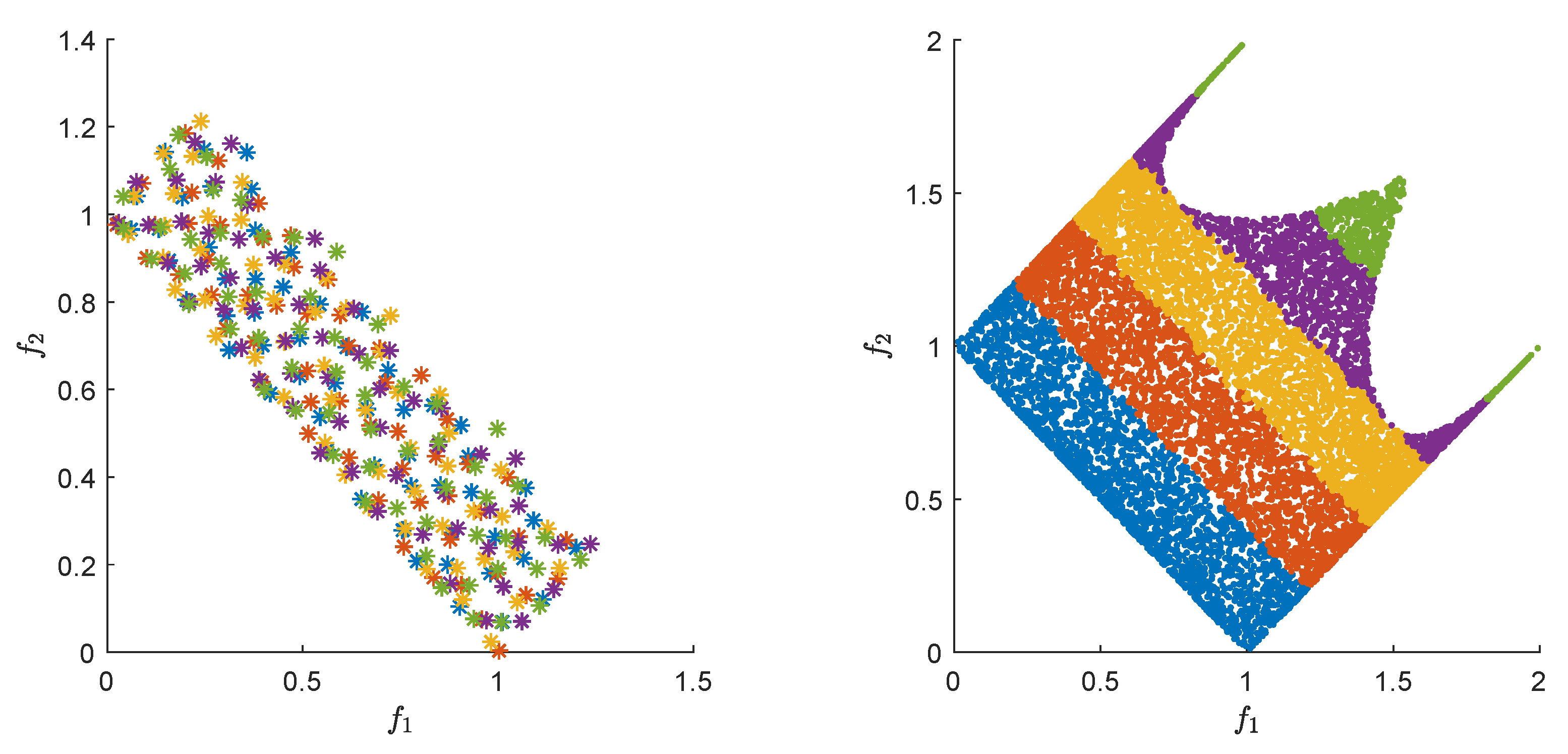
Figure 1 shows the different fronts formed with different colors. It is possible to observe that the use of ${\delta }_y$ and ${\delta }_x$ allows for a criterion to decide between solutions that are non $-ϵ$-dominated, while, in the bottom figure, all solutions in blue would belong to the first front. Meanwhile, in the upper figure, there are fewer solutions, and their rank is decided by how well-spaced they are in both spaces. This feature is important since it would be possible to add a preference on the rank by the spacing between solutions.

Figure 1. Ranking nearly optimal solutions for the first five ranks on Lamé superspheres MOP (LSS) with $\alpha =0.5$ [54]. The figure shows the rankings with the proposed algorithm that uses ${\delta }_y$ (left) and without (right).

4.3. Using Subpopulations

Since the $-ϵ$-dominance can be viewed as a relaxed form of Pareto dominance, it can be expected that more solutions are non $-ϵ$-dominated when compared to classical dominance. This fact generates a potential issue since it would be possible that the algorithm stagnates at the early stages.

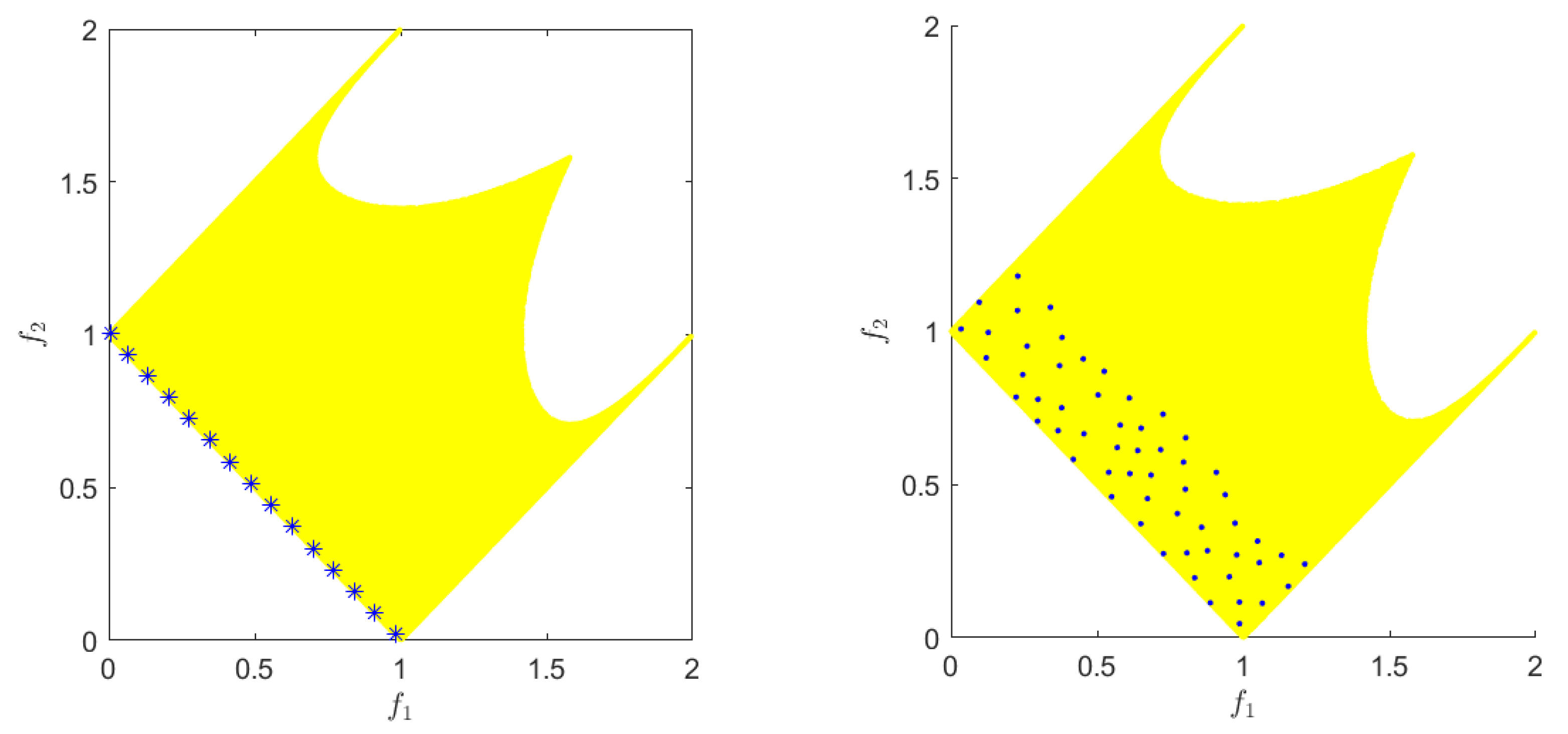
To avoid this issue, we propose the use of two subpopulations to improve the pressure towards the set of interest of the novel algorithm. Each subpopulation has a different aim. The first one aims to approximate the global Pareto set/front. While the second one seeks to approximate $P_{Q,ϵ}$. Figure 2 shows what would be the first rank for each subpopulation. A vital aspect of the approach is how the information between the subpopulations is shared. Thus, in the following, we describe two schemes to share individuals via migration.

Figure 2. The figure shows in yellow the feasible space and in blue the first rank for each subpopulation on LSS with $\alpha =0.5$—on the left, the first ranked solutions that aim for the global Pareto front, on the right, the first ranked solutions that aim for the set of approximate solutions.

• Migration: every $nf$ generations, $nr$ individuals are exchanged between the population. The individuals are chosen at random from the rank one individuals.
• Crossover between subpopulations: every $nf$ generations, the crossover is performed between the populations. One parent is chosen from each population at random.

As it can be observed, the use of subpopulations introduces three extra parameters to the algorithm, namely:

• $nf$: frequency of migration,
• $nr$: the number of individuals to be exchanged, and
• $ratio$: the ratio of individuals between subpopulation in the range $[0,1]$.

Thus, the population in charge of looking for optimal solutions puts pressure on the second population and helps to determine the set of approximate solutions. While the latter population is in charge of exploiting the promissory regions, this allows for finding local Pareto fronts if they are `close enough’ in terms of $-ϵ$-dominance.

4.4. Complexity of the Novel Algorithm

In the following, we comment on the complexity of N$ϵ$SGA. Let G be the number of generations and $\left|P\right|$ the size of the population.

• Initialization: in this step, all the individuals are generated at random and evaluated. This task takes $O\left(\right|P\left|\right)$.
• External archiver: from the previous section, the complexity of the archiver is $O\left(\right|P\left|\right|A\left|\right)$, where $\left|A\right|$ is the size of the archiver. Note that the maximum size of the archiver at the end of the execution is $G\left|P\right|$.
• Non $ϵ$-dominated sorting: until there are no solutions in the population P, $ArchiveUpdate{P}_{Q,ϵ}{D}_{xy}$ is executed. In the worst case, each rank has only one solution, and the archiver is executed $\left|P\right|$ times. Thus, the complexity of this part of the algorithm is $O\left(\right|P{|}^3)$.
• Main loop: the main loop selects the parents and applies the genetic operators (each of this tasks take $O\left(\right|P\left|\right)$), then the algorithm uses the Non $ϵ$-dominated sorting ($O\left(\right|P{|}^3)$); next, it finds those solutions that are well distributed in terms of closest neighbor ($O\left(\right|P{|}^2)$) and finally applies the external archiver $O\left(\right|P{|}^2)$. Note that all these operations are executed G times. Thus, the complexity of the algorithm is ${O\left(max\right(G\left|P\right|}^3,{\left(G\right|P\left|\right)}^2\left)\right)$, which is the maximum of the non $ϵ$-dominated sorting or the external archiver.

5. Numerical Results

In this section, we present the numerical result coxrresponding to the evolutionary algorithm. We performed several experiments to validate the novel algorithm. First, we validate the use of an external archiver in the evolutionary algorithm. Next, we compare several strategies of subpopulations. Finally, we analyze the resulting algorithm with the enhanced state-of-the-art algorithms.

The algorithms chosen are modifications of $P_{Q,ϵ}$NSGA-II, and $P_{Q,ϵ}$MOEA. In the literature, both algorithms used aim for well-distributed solutions only in objective space, but, in this case, we enhanced them with $ArchiverUpdate{P}_{Q,ϵ}{D}_{xy}$ to have a fair comparison with the proposed algorithm.

In all cases, we used the following problems: Deb99 [17], two-on-one [55], sym-part [44], S. Schäffler, R. Schultz and K. Weinzierl (SSW) [56], omni test [53], Lamé superspheres (LSS) [54]. Next, 20 independent experiments were performed with the following parameters: 100 individuals, 100 generations, crossover rate = $0.9$, mutation rate = $1/n$, distribution index for crossover $eta\_c=20$ and distribution index for mutation $eta\_m=20$. Then, Table 1 shows the $ϵ$, ${\delta }_y$ and ${\delta }_x$ values used for each problem. Furthermore, all cases were measured with the ${\Delta }_2$ indicator, and a Wilcoxon rank-sum test was performed with a significance level $\alpha =0.05$. Finally, all ${\Delta }_2$ tables, the bold font represents the best mean value, and the arrows represent:

Table 1. Parameters used for the experiments.

Problem	$\mathit{ϵ}$	${\mathit{\delta }}_{\mathit{y}}$	${\mathit{\delta }}_{\mathit{x}}$	Domain
Deb99	[0.011, 0.011]	[0.2, 0.2]	[0.2, 0.2]	$x\in {[0.01,1]}^2$
Two-on-one	[0.1, 0.1]	[0.1, 0.1]	[0.02, 0.2]	$x\in {[-10,10]}^2$
Sym-part	[0.15, 0.15]	[0.2, 0.1]	[1, 1]	$x\in {[-20,20]}^2$
SSW n=3	[0.011, 0.0001]	$\frac{1}{3}ϵ$	[1, 1, 1]	$x\in {[0,40]}^3$
Omni-test	[0.01, 0.01]	[0.05, 0.05]	[0.1, 0.1, 0.1, 0.1 ]	$x\in {[0,6]}^5$
LSS	[0.1, 0.1]	[0.05, 0.05]	[0.1, 0.1, 0.1, 0.1, 0.1]	$x\in [0,\pi /2]\times {[1,5]}^4$

• ↑ rank sum rejects the null hypothesis of equal medians and the algorithm has a better median,
• ↓ rank sum rejects the null hypothesis of equal medians, and the algorithm has a worse median and
• ↔ rank sum cannot reject the null hypothesis of equal medians.

The comparison is always made with the algorithm in the first column. We have selected the ${\Delta }_2$ indicator since it allows us to compare the distance between the reference solution and the approximation found by the algorithms in both decision and objective space. Since we aim to compute the set of approximate solutions, classical indicators used to measure Pareto fronts cannot be applied in a straightforward manner and should be carefully studied if one would like to use them in this context.

5.1. Validation of the Use of an External Archiver

We first validate the use of an external archiver in the novel algorithm. Note N$ϵ$SGA2A denotes the version of the algorithm that uses the external archiver. Table 2 and Table 3 show the mean and standard deviation of the ${\Delta }_2$ values obtained by the algorithms. From the results, we can observe that in the six problems the use of the external archiver has a significant impact on the algorithm. This indicates an advantage of using the novel archiver. It is important to notice that the use of the external archiver does not use any function evaluation. Thus, the comparison is fair regarding the number of evaluations used.

Table 2. Averaged ${\Delta }_2$ in decision space for the use of the external archiver and the base case.

Problem	N$\mathit{ϵ}$SGA2	N$\mathit{ϵ}$SGA2-A
Deb99	0.0621 (0.0040)	0.0316 (0.0129)↑
Two-on-one	0.1125 (0.1397)	0.0595 (0.1467)↑
Sym-part	0.2466 (0.0242)	0.0741 (0.0039)↑
SSW	2.9840 (0.2123)	1.0050 (0.0226)↑
Omni test	1.5740 (0.1163)	0.8680 (0.2806)↑
LSS	1.5092 (0.0532)	0.6415 (0.0163)↑

Table 3. Averaged ${\Delta }_2$ in objective space for the use of the external archiver and the base case.

Problem	N$\mathit{ϵ}$SGA2	N$\mathit{ϵ}$SGA2-A
Deb99	0.1436(0.0254)	0.0255(0.0015)↑
Two-on-one	0.9771(0.1385)	0.2726(0.2522)↑
Sym-part	0.3147(0.0116)	0.1232(0.0087)↑
SSW	0.7916(0.0908)	0.2128(0.0016)↑
Omni test	0.0513(0.0047)	0.0203(0.0061)↑
LSS	0.1610(0.0079)	0.0222(0.0036)↑

5.2. Validation of the Use of Subpopulations

Furthermore, we experiment with whether the use of subpopulations in the novel algorithm has a positive effect on the algorithm. N$ϵ$SGA2Is1 denotes the approach that uses migration, and N$ϵ$SGA2Is2 denotes the approach that uses a crossover between the subpopulations. Table 4 and Table 5 show the mean and standard deviation of the ${\Delta }_2$ values obtained by the algorithms. From the results, we can observe that the approach that uses migration is outperformed in four of the twelve comparisons (considering both decision and objective space). On the other hand, the approach that uses crossover between subpopulations is outperformed by the base algorithm in three of twelve comparisons. As it could be expected, the algorithms that use subpopulations obtain better results in terms of objective space while sacrificing in some cases decision space.

Table 4. Averaged ${\Delta }_2$ for the algorithms that use subpopulations and the base case in decision space.

Problem	N$\mathit{ϵ}$SGA2	N$\mathit{ϵ}$SGA2-Is1	N$\mathit{ϵ}$SGA2-Is2
Deb99	0.0316 (0.0129)	0.0290 (0.0182)↔	0.0370 (0.0170)↔
Two-on-one	0.0595 (0.1467)	0.0925 (0.2025)↔	0.0266 (0.0003)↔
Sym-part	0.0741 (0.0039)	0.0597 (0.0034)↑	0.0621 (0.0061)↑
SSW	1.0050 (0.0226)	1.0402 (0.0279)↓	1.0554 (0.0179)↓
Omni test	0.8680 (0.2806)	1.0647 (0.3026)↓	0.9321 (0.2316)↔
LSS	0.6415 (0.0163)	0.6657 (0.0109)↓	0.6917 (0.0219)↓

Table 5. Averaged ${\Delta }_2$ for the algorithms that use subpopulations and the base case in objective space.

Problem	N$\mathit{ϵ}$SGA2	N$\mathit{ϵ}$SGA2-Is1	N$\mathit{ϵ}$SGA2-Is2
Deb99	0.0255 (0.0015)	0.0369 (0.0173)↓	0.0444 (0.0431)↓
Two-on-one	0.2726 (0.2522)	0.3004 (0.3565)↔	0.1874 (0.0659)↑
Sym-part	0.1232 (0.0087)	0.0884 (0.0108)↑	0.0943 (0.0170)↑
SSW	0.2128 (0.0016)	0.2116 (0.0020)↑	0.2109 (0.0029)↑
Omni test	0.0203 (0.0061)	0.0198 (0.0063)↔	0.0209 (0.0044)↔
LSS	0.0222 (0.0036)	0.0145 (0.0043)↑	0.0156 (0.0029)↑

5.3. Comparison to State-of-the-Art Algorithms

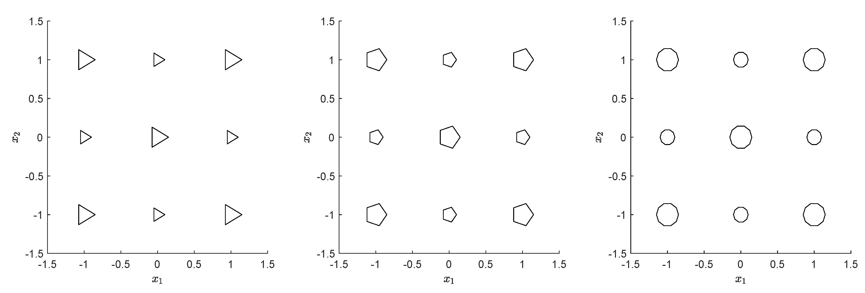
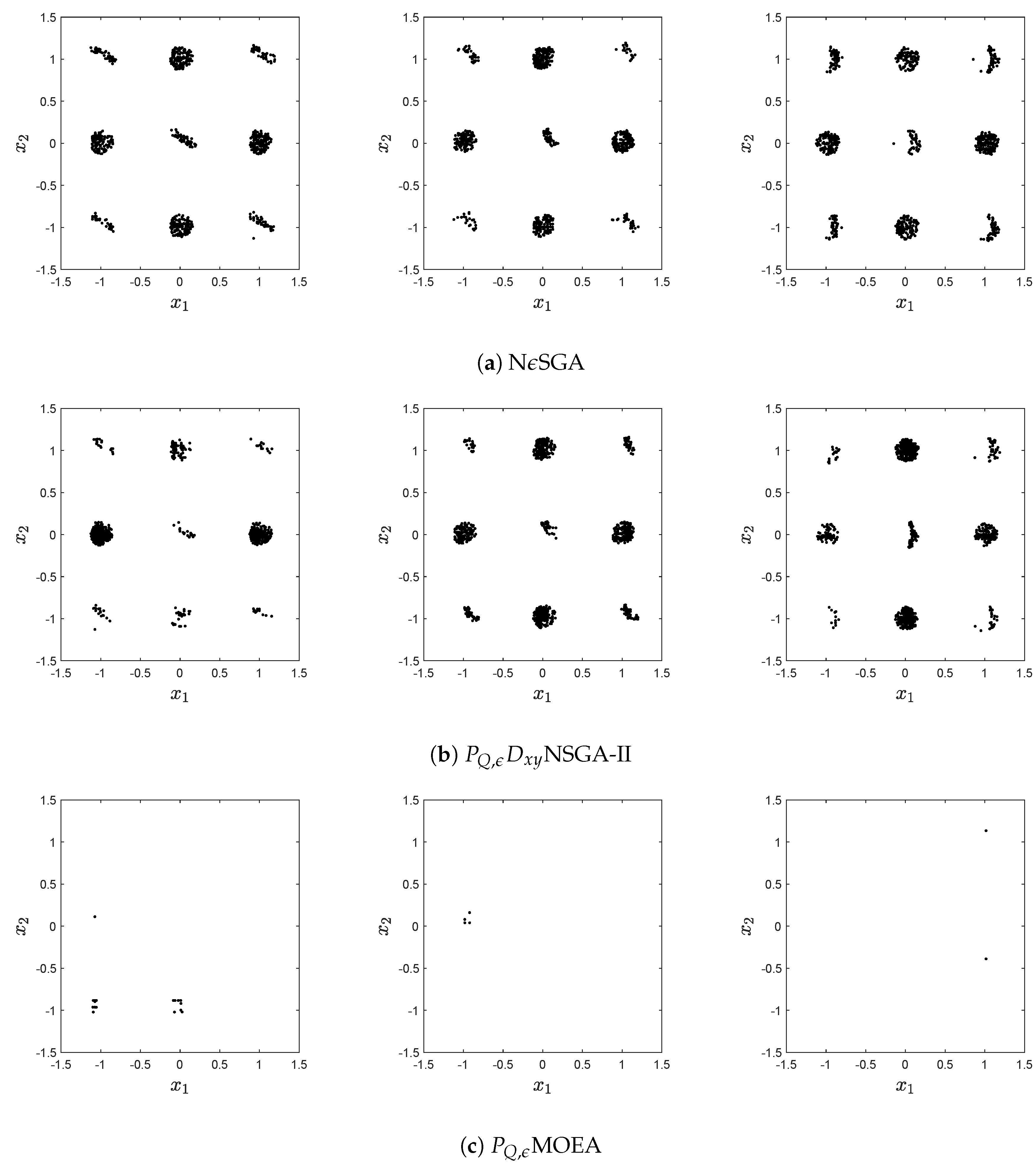
Now, we compare the proposed algorithm with $P_{Q,ϵ}{D}_{xy}$-NSGA2 and $P_{Q,ϵ}{D}_{xy}$-MOEA. Additionally to the MOPs used previously, in this section, we consider three distance-based multi/many-objective point problems (DBMOPP) [50,51,57]. These problems allow us to visually examine the behavior of many-objective evolution as they can scale on the number of objectives. In this context, there are K sets of vectors defined, where the kth set, $V_k=\{v_1,\dots ,v_{m_k}\}$ determines the quality of a design vector $x\in Q$ on the kth objective. This can be computed as

$$f_k\left(x\right)=\underset{v\in V_k}{min}\left(dist(x,v)\right),$$

(7)

where $m_k$ is the number of elements of $V_k$, which depends on k and $dist(x,v)$ denotes in the Euclidian distance. An alternative representation is given by the centre (c), a circle radius (r), and an angle for each objective minimizing vector. From this framework, we generate three problems with $k=3,5,10$ objectives. Each problem has nice connected components with centers $c=\left[\right[-1,-1],[-1,0],[-1,1],[0,-1],[0,0],[0,1],[1,-1],[1,0],[1,1\left]\right]$. Furthermore, the radius $r=[0.15,0.1,0.15,0.15,0.1,0.15,0.15,0.1,0.15]$ and the angle $a=[a_i:a_i\in \frac{2i\pi }{k}]$ for $i=1,\dots ,k$. 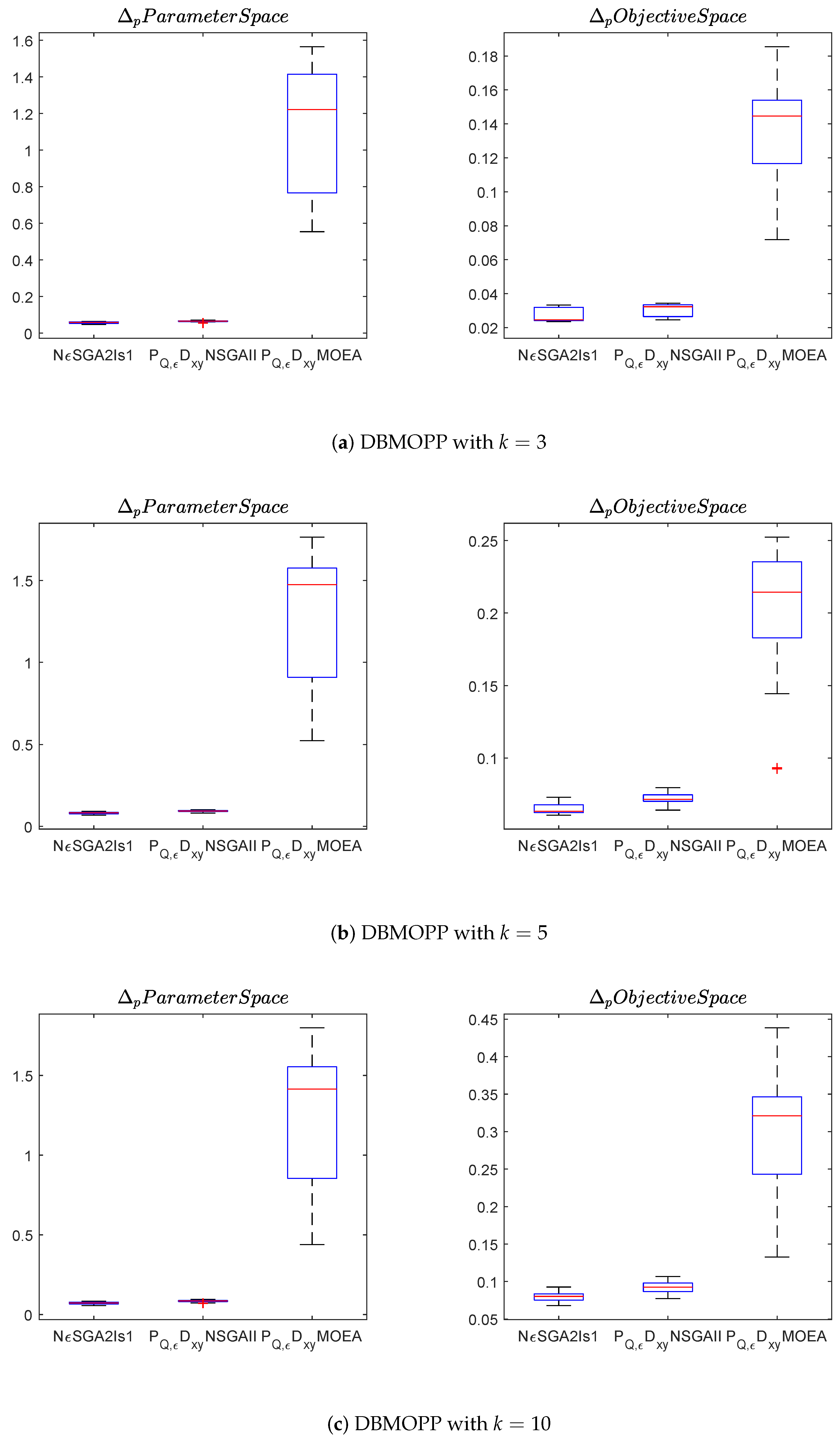Figure 3 shows the structure for each problem. Each polygon represents a local Pareto set. The global Pareto sets are those centered in $\left[\right[-1,0],[0,-1],[0,1],[1,0\left]\right]$. For these problems, we used $ϵ={[0.05]}^k$, ${\delta }_x=[0.02,0.02]$, ${\delta }_y={[0.01]}^k$ and $-10\le x_1,x_2\le 10$.

Figure 3. Local Pareto set regions of the DBMOPP problems generated for $k=3,5,10$ objectives.

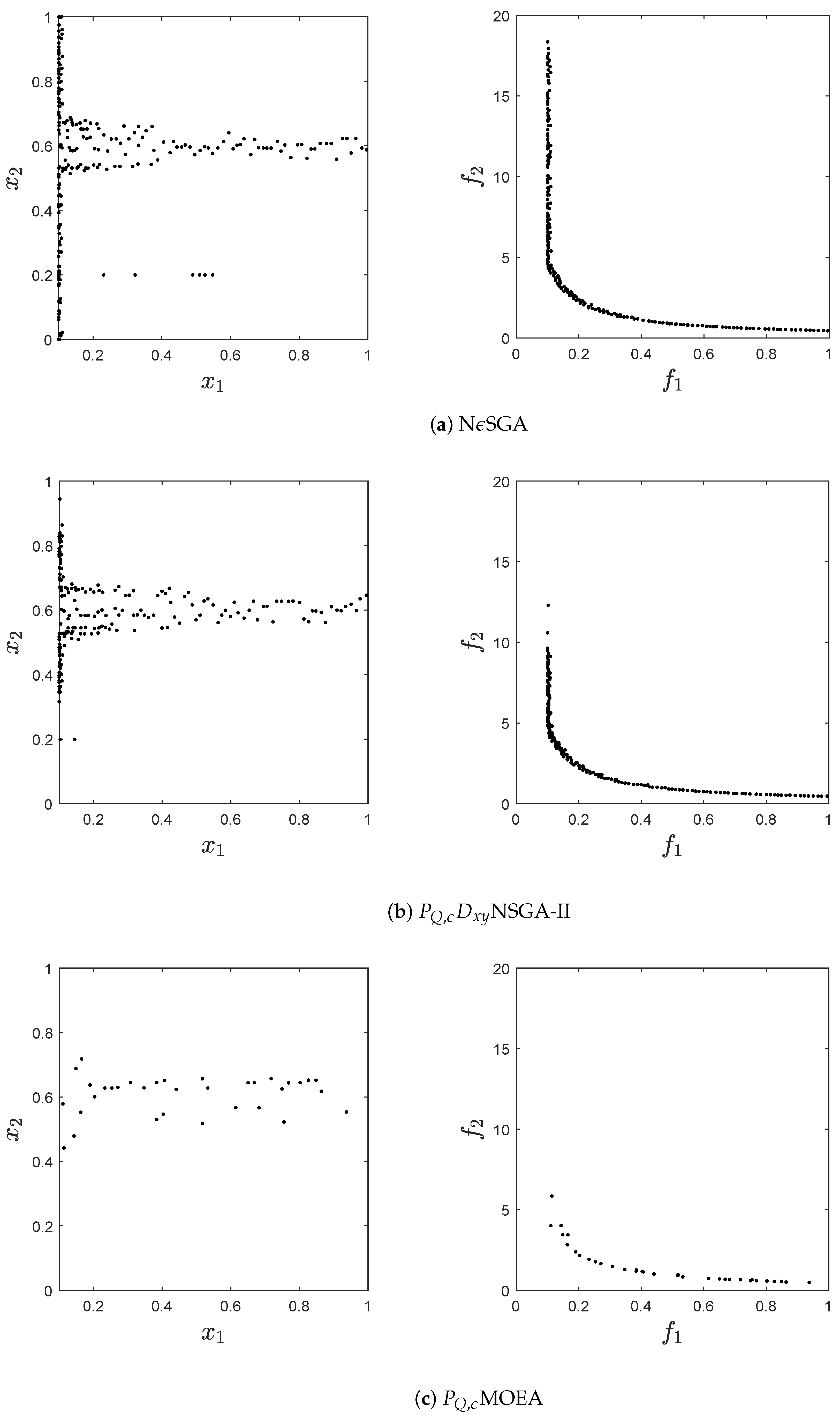
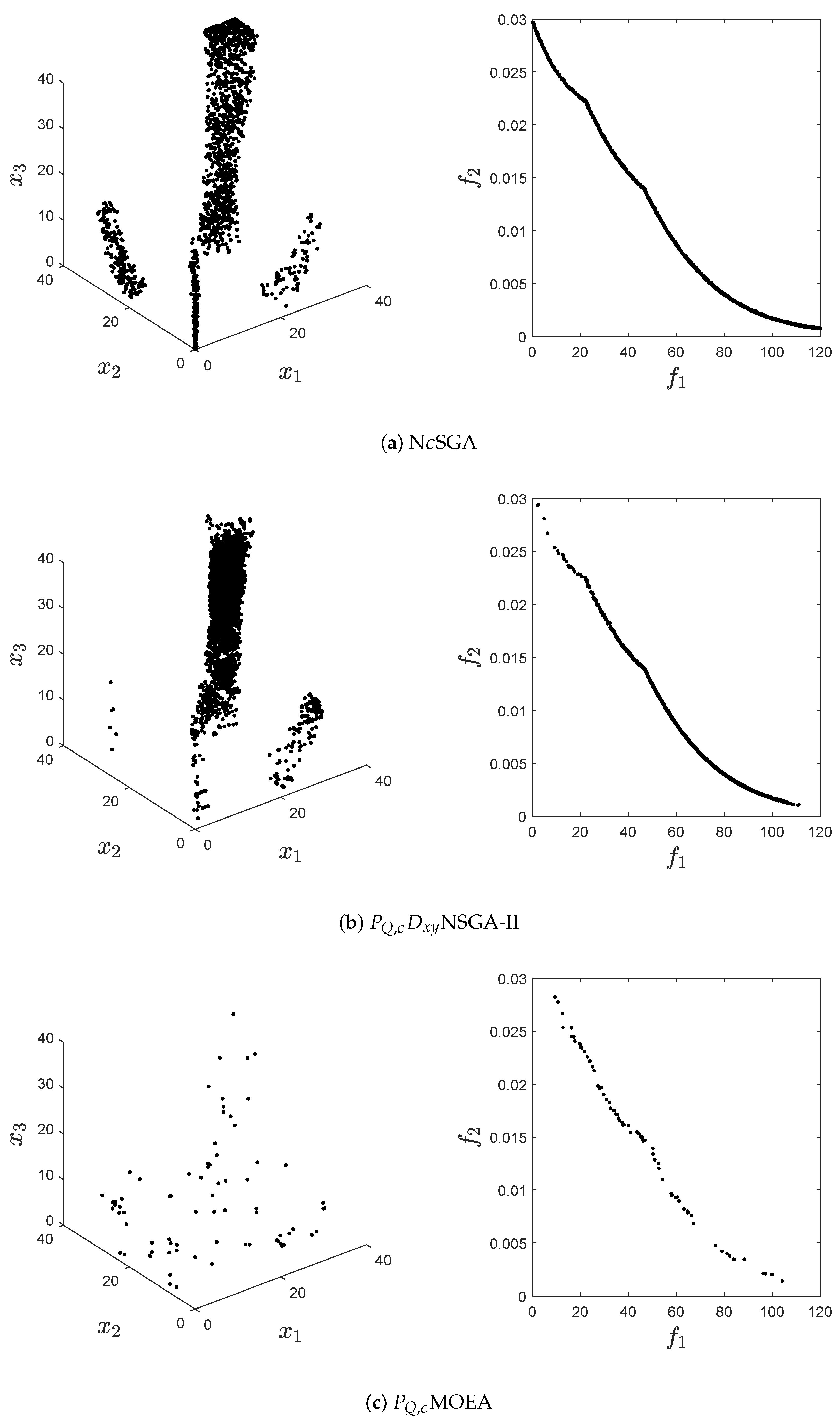
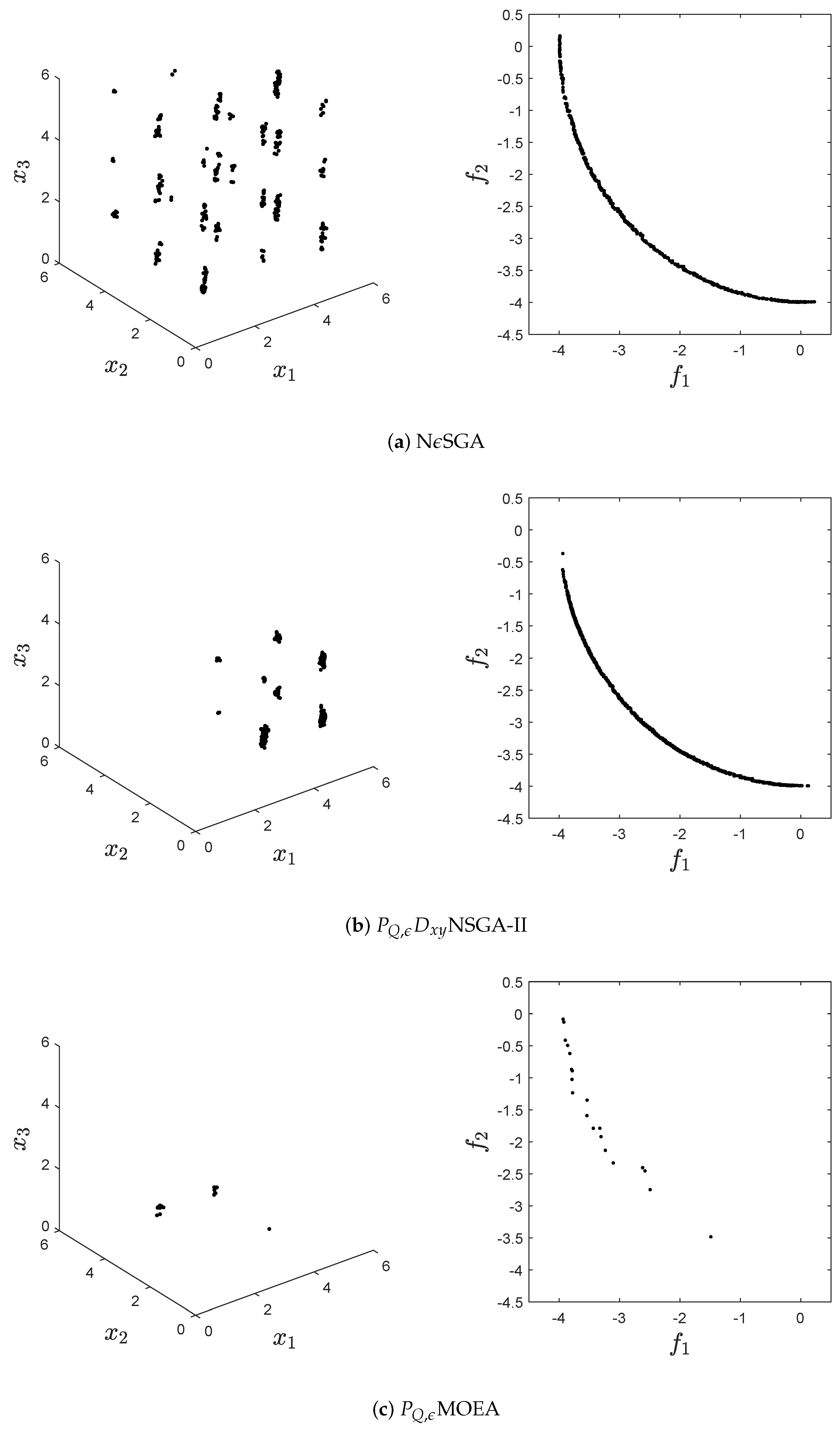
Figure 4, Figure 5, Figure 6 and Figure 7 show the median approximations to $P_{Q,ϵ}$ and $F\left(P_{Q,ϵ}\right)$ obtained by the algorithms. It is posible to observe than in all figures $P_{Q,ϵ}{D}_{xy}$-MOEA has the worst performance. Next, $P_{Q,ϵ}{D}_{xy}$-NSGA2 misses several connected components that are of the set of approximate solutions. Figure 6 shows a clear example where $P_{Q,ϵ}{D}_{xy}$-NSGA2 focuses on a few regions of the decision space while the proposed algorithm is capable of finding all connected components. 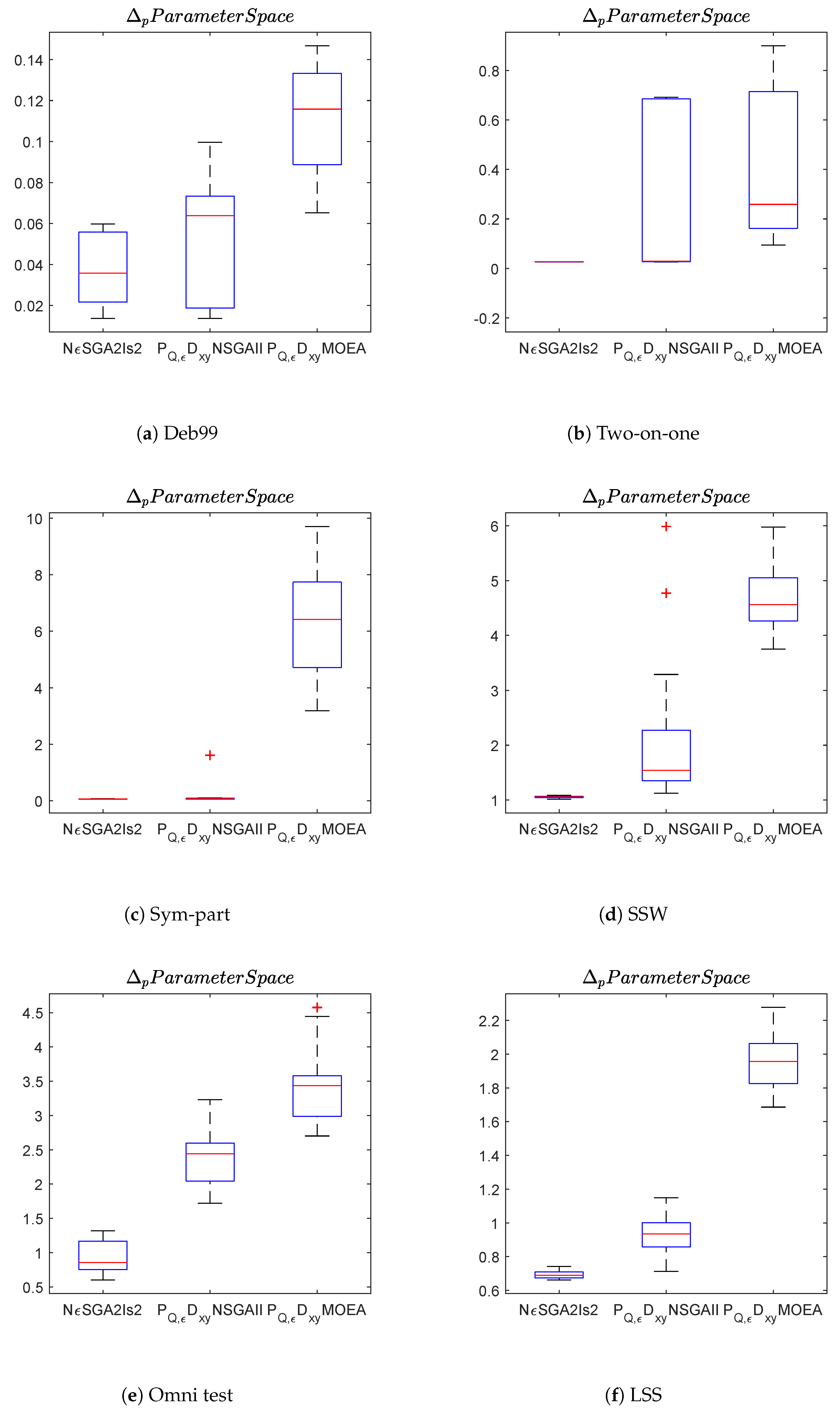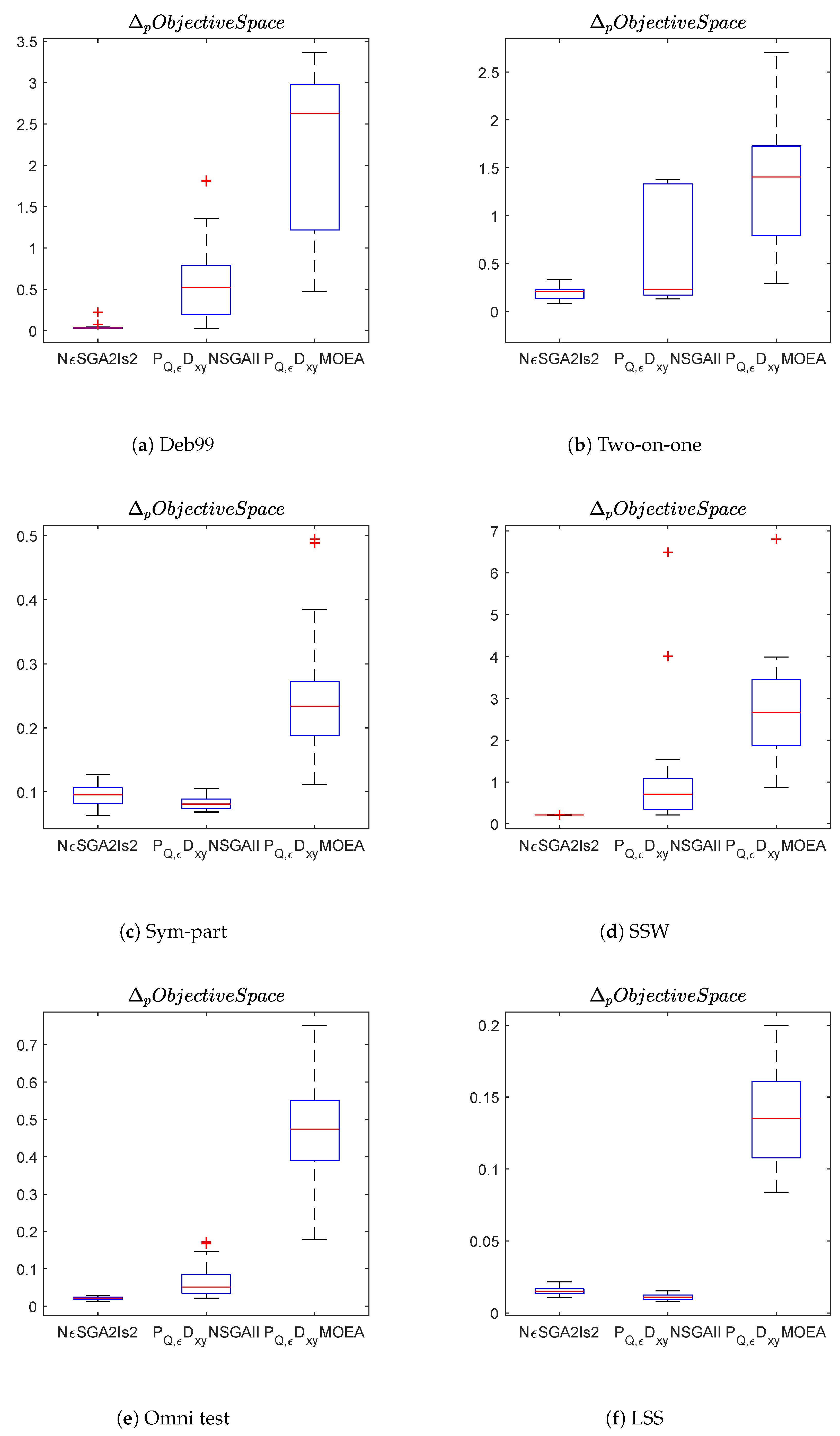Furthermore, Figure 8, Figure 9 and Figure 10 show the box plots in both decision and objective space for the problems considered. Table 6 and Table 7 show the mean and standard deviation of the ${\Delta }_2$ values obtained by the algorithms.

Figure 4. Numerical results on Deb99 for the comparison of N$ϵ$SGA2 and the state-of-the-art algorithms.

Figure 5. Numerical results on SSW for the comparison of N$ϵ$SGA2 and the state-of-the-art algorithms.

Figure 6. Numerical results on Omni test for the comparison of N$ϵ$SGA2 and the state-of-the-art algorithms.

Figure 7. Numerical results on DBMOPPs for the comparison of N$ϵ$SGA2 and the state-of-the-art algorithms.

Figure 8. Box plots of ${\Delta }_2$ in decision space of N$ϵ$SGA, $P_{Q,ϵ}{D}_{xy}$-NSGA-II and $P_{Q,ϵ}{D}_{xy}$-MOEA/D from left to right.

Figure 9. Box plots of ${\Delta }_2$ in objective space of N$ϵ$SGA, $P_{Q,ϵ}{D}_{xy}$-NSGA-II and $P_{Q,ϵ}{D}_{xy}$-MOEA/D from left to right.

Figure 10. Box plots of ${\Delta }_2$ in decision space (left) and objective space (right) of N$ϵ$SGA, $P_{Q,ϵ}{D}_{xy}$-NSGA-II and $P_{Q,ϵ}{D}_{xy}$-MOEA/D.

Table 6. Averaged ${\Delta }_2$ in decision space for the comparison of the state-of-the-art algorithms.

Problem	N$\mathit{ϵ}$SGA2-Is2	${\mathit{P}}_{\mathit{Q},\mathit{ϵ}}{\mathit{D}}_{\mathbf{xy}}$-NSGA-II	${\mathit{P}}_{\mathit{Q},\mathit{ϵ}}{\mathit{D}}_{\mathbf{xy}}$-MOEA/D
Deb99	0.0370 (0.0170)	0.0513 (0.0294)↓	0.1106 (0.0258)↓
Two-on-one	0.0266 (0.0003)	0.2585 (0.3222)↓	0.4298 (0.2913)↓
Sym-part	0.0621 (0.0061)	0.2238 (0.4746)↔	6.2978 (2.0763)↓
SSW	1.0554 (0.0179)	2.0611 (1.2699)↓	4.6774 (0.5790)↓
Omni test	0.9321 (0.2316)	2.3839 (0.3911)↓	3.4810 (0.5715)↓
LSS	0.6917 (0.0219)	0.9327 (0.1048)↓	1.9653 (0.1701)↓
DBMOPP $k=3$	0.0577(0.0047)	0.0648(0.0032)↓	1.1303(0.3411)↓
DBMOPP $k=5$	0.0811(0.0068)	0.0937(0.0050)↓	1.2928(0.3677)↓
DBMOPP $k=10$	0.0720(0.0074)	0.0843(0.0064)↓	1.2342(0.4304)↓

Table 7. Averaged ${\Delta }_2$ in objective space for the comparison of the state-of-the-art algorithms.

Problem	N$\mathit{ϵ}$SGA2-Is2	${\mathit{P}}_{\mathit{Q},\mathit{ϵ}}{\mathit{D}}_{\mathbf{xy}}$-NSGA-II	${\mathit{P}}_{\mathit{Q},\mathit{ϵ}}{\mathit{D}}_{\mathbf{xy}}$-MOEA/D
Deb99	0.0444 (0.0431)	0.6283 (0.5474)↓	2.1702 (1.0106)↓
Two-on-one	0.1874 (0.0659)	0.5932 (0.5664)↓	1.3167 (0.6075)↓
Sym-part	0.0943 (0.0170)	0.0826(0.0106)↑	0.2524 (0.0996)↓
SSW	0.2109 (0.0029)	1.1394 (1.5114)↓	2.7317 (1.2801)↓
Omni test	0.0209 (0.0044)	0.0685 (0.0491)↓	0.4762 (0.1264)↓
LSS	0.0156 (0.0029)	0.0109(0.0021)↑	0.1369 (0.0349)↓
DBMOPP $k=3$	0.0267(0.0038)	0.0305(0.0036)↓	0.1352(0.0315)↓
DBMOPP $k=5$	0.0647(0.0033)	0.0717(0.0038)↓	0.2005(0.0466)↓
DBMOPP $k=10$	0.0798(0.0070)	0.0919(0.0080)↓	0.2972(0.0773)↓

From the results, we can observe that the novel algorithm outperforms $P_{Q,ϵ}{D}_{xy}$-NSGA2 in eight out of nine problems according to decision space and seven according to objective space. When compared with $P_{Q,ϵ}{D}_{xy}$-MOEA, the novel algorithm outperforms in the nine problems according to both decision and objective space. This shows that an improvement in the search engine to maintain solutions well spread in decision and objective space is advantageous when approximating $P_{Q,ϵ}$.

To conclude the comparison to state-of-the-art algorithms, we aggregate the results by conducting a single election winner strategy. Here, we have selected the Borda and Condorcet methods to perform our analysis [58].

In the Borda method, for each ranking, assign to algorithm X, the number of points equal to the number of algorithms it defeats. In the Condorcet method, if algorithm A defeats every other algorithm in a pairwise majority vote, then A should be ranked first. Table 8 shows that the count of times algorithm i was significantly better than the algorithm j according to the Wilcoxon rank sum. In this case, both Borda count and Condorcet method prefer the novel method. Furthermore, in terms of computational complexity, both state-of-the-art methods have a complexity of ${O\left(\right(G\parallel P\parallel )}^2)$ since both algorithms make use of the external archiver. This complexity is comparable with the one of the novel method. In some cases, due to the non $ϵ$-dominated sorting, the novel algorithm can have a higher complexity.

Table 8. Summary of times a method outperforms another with statistical significance.

Method	N$\mathit{ϵ}$SGA	${\mathit{P}}_{\mathit{Q},\mathit{ϵ}}$-NSGA2	${\mathit{P}}_{\mathit{Q},\mathit{ϵ}}$-MOEA	Borda Count
N$ϵ$SGA	0	15	18	32
$P_{Q,ϵ}$-NSGA2	2	0	18	20
$P_{Q,ϵ}$-MOEA	0	0	0	0

5.4. Application to Non-Uniform Beam

Finally, we consider a non-uniform beam problem taken from [59,60]. Non-uniform beams are a commonly used structure in many applications such as ship hull, rocket surface, and aircraft fuselage. In this application, structural and acoustic properties are presented as constraints and performance indices of candidate non-uniform beams.

The primary goal of the structural-acoustic design is to create a light-weight, stable, and quiet structure. The multi-objective optimization of non-uniform beams is to seek the balance among those aims. Here, we will consider the following bi-objective problem:

The first objective $\overline{P}$ is the integration of the radiated sound power over a range of frequencies,

$$\overline{P}={\int }_{200}^{600}Pd\omega ,$$

(8)

where P is the average acoustic power radiated by the vibrating beam per unit width over one period of vibrations (see [60] for the details of the implementation).

The second objective is the total mass of the beam that can be expressed as

$$m_{tot}={\displaystyle \sum _{n=1}^N}\frac{\rho h_{i}L}{N},$$

(9)

where $1\le h_i\left(x\right)\le 15$ mm is the average height of the ith segment, and for the number of interpolation coordinates $N=10$ (i.e., the decision space is 10-dimensional). The Beam length is $L=1.0$ m and the mass density $\rho =2643{\mathrm{kg}/\mathrm{m}}^3$.

The parameters for the archiver were set to $ϵ=[1,0.00003]$, ${\delta }_x=2.5\times {10}^{-3}$ and ${\delta }_y=[0.3,0.000003]$. That is to say, we are willing to accept a deterioration of 1 kg and $0.3\times {10}^{-5}$ W/m/s.

The parameters were as follows:

• Population size: 500,
• Number of generations: 200,
• The rest of the parameters were set as before.

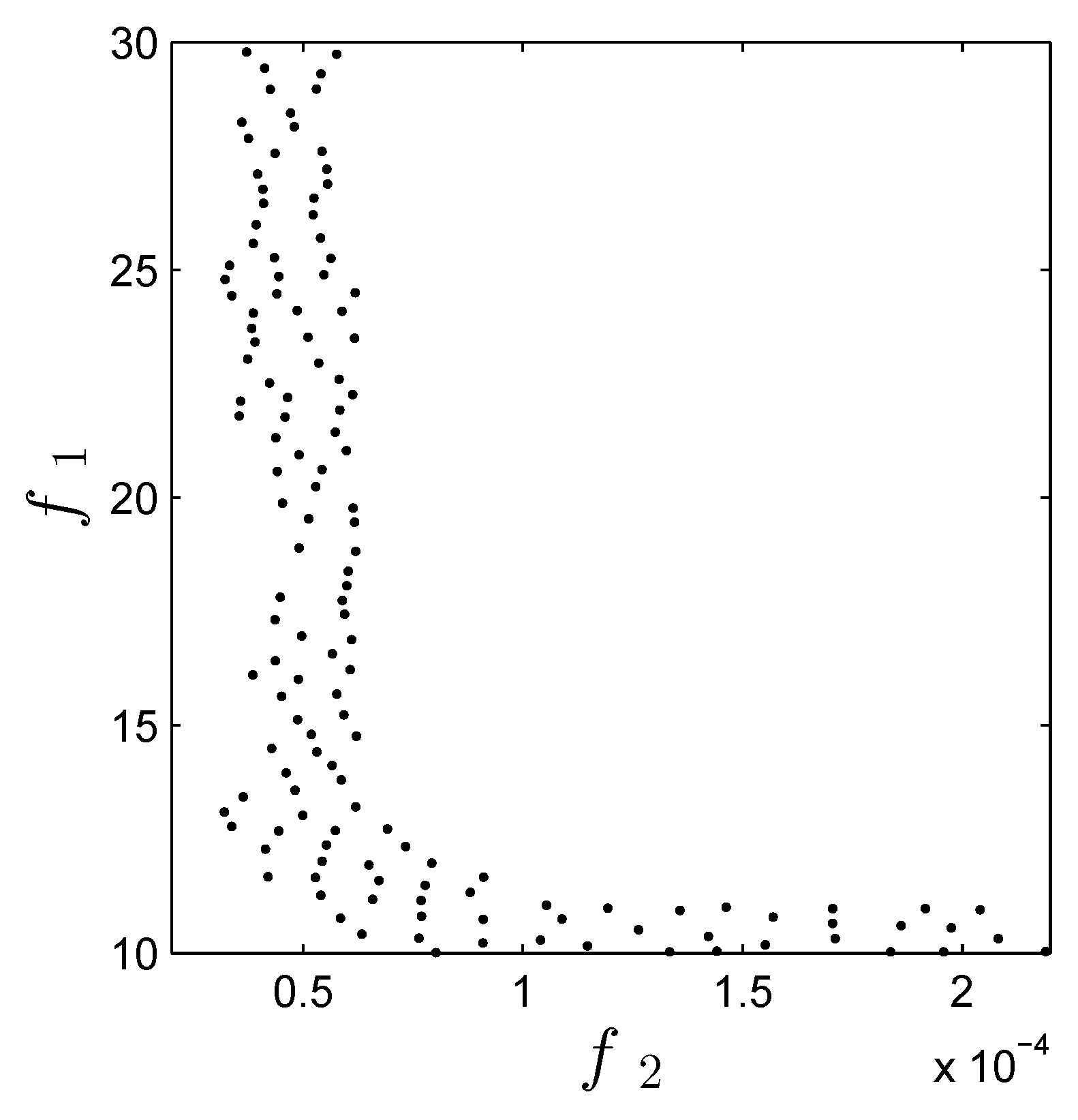
Figure 11 shows the approximated set $P_{Q,ϵ}$. The results show that the algorithm is capable of finding the region of interest, according to previous studies [19,60], with $100,000$ function evaluations, while in previous work using only the archiver with random points, it took 10 million function evaluations [19] to obtain similar results.

Figure 11. Approximation of $P_{Q,ϵ}$ obtained with N$ϵ$SGA

6. Conclusions and Future Work

In this work, we have proposed a novel multi-objective evolutionary algorithm that aims to compute the set of approximate solutions. The algorithm uses the archiver $Archive{P}_{Q,ϵ}{D}_{xy}$ to maintain a well-distributed representation in both decision and objective space. Moreover, the algorithm ranks the solutions according to the $-ϵ$-dominance and their distribution in both decision and objective space. This allows exploring different regions of the search space where approximate solutions might be located and maintaining them in the archiver.

Furthermore, we observed that the interplay of generator and archiver was a delicate problem, including (among others) a proper balance of local/global search, a suitable density distribution for all generational operators. The results show that the novel algorithm is competitive against other methods of the-state-of-the-art on academic problems. Finally, we applied the algorithm to an optimal control problem with comparable results to those of the state-of-the-art but using significantly fewer resources.

References

- Hernández, C.; Naranjani, Y.; Sardahi, Y.; Liang, W.; Schütze, O.; Sun, J.Q. Simple cell mapping method for multi-objective optimal feedback control design. Int. J. Dyn. Control 2013, 1, 231–238. [Google Scholar] [CrossRef]
- Sardahi, Y.; Sun, J.Q.; Hernández, C.; Schütze, O. Many-Objective Optimal and Robust Design of Proportional-Integral-Derivative Controls with a State Observer. J. Dyn. Syst. Meas. Control 2017, 139, 024502. [Google Scholar] [CrossRef]
- Zakrzewska, A.; d’Andreagiovanni, F.; Ruepp, S.; Berger, M.S. Biobjective optimization of radio access technology selection and resource allocation in heterogeneous wireless networks. In Proceedings of the 2013 11th International Symposium and Workshops on Modeling and Optimization in Mobile, Ad Hoc and Wireless Networks (WiOpt), Tsukuba Science City, Japan, 13–17 May 2013; pp. 652–658. [Google Scholar]
- Andrade, A.R.; Teixeira, P.F. Biobjective optimization model for maintenance and renewal decisions related to rail track geometry. Transp. Res. Record 2011, 2261, 163–170. [Google Scholar] [CrossRef]
- Stepanov, A.; Smith, J.M. Multi-objective evacuation routing in transportation networks. Eur. J. Op. Res. 2009, 198, 435–446. [Google Scholar] [CrossRef]
- Meskens, N.; Duvivier, D.; Hanset, A. Multi-objective operating room scheduling considering desiderata of the surgical team. Decis. Support Syst. 2013, 55, 650–659. [Google Scholar] [CrossRef]
- Dibene, J.C.; Maldonado, Y.; Vera, C.; de Oliveira, M.; Trujillo, L.; Schütze, O. Optimizing the location of ambulances in Tijuana, Mexico. Comput. Biol. Med. 2017, 80, 107–115. [Google Scholar]
- Beyer, H.G.; Sendhoff, B. Robust optimization—A comprehensive survey. Comput. Methods Appl. Mech. Eng. 2007, 196, 3190–3218. [Google Scholar] [CrossRef]
- Jin, Y.; Branke, J. Evolutionary optimization in uncertain environments—A survey. IEEE Trans. Evol. Comput. 2005, 9, 303–317. [Google Scholar] [CrossRef]
- Deb, K.; Gupta, H. Introducing Robustness in Multi-Objective Optimization. Evol. Comput. 2006, 14, 463–494. [Google Scholar] [CrossRef]
- Avigad, G.; Branke, J. Embedded Evolutionary Multi-Objective Optimization for Worst Case Robustness. In Proceedings of the 10th Annual Conference on Genetic and Evolutionary Computation, GECCO ’08, Atlanta, GA, USA, 12–16 July 2008; pp. 617–624. [Google Scholar] [CrossRef]
- Loridan, P. ϵ-Solutions in Vector Minimization Problems. J. Optim. Theory Appl. 1984, 42, 265–276. [Google Scholar] [CrossRef]
- Schütze, O.; Esquivel, X.; Lara, A.; Coello Coello, C.A. Using the Averaged Hausdorff Distance as a Performance Measure in Evolutionary Multi-Objective Optimization. IEEE Trans. Evol. Comput. 2012, 16, 504–522. [Google Scholar] [CrossRef]
- Pareto, V. Manual of Political Economy; The MacMillan Press: New York, NY, USA, 1971. [Google Scholar]
- Hillermeier, C. Nonlinear Multiobjective Optimization—A Generalized Homotopy Approach; Birkhäuser: Basel, Switzerland, 2001. [Google Scholar]
- White, D.J. Epsilon efficiency. J. Optim. Theory Appl. 1986, 49, 319–337. [Google Scholar] [CrossRef]
- Deb, K. Multi-Objective Optimization Using Evolutionary Algorithms; John Wiley & Sons: Chichester, UK, 2001. [Google Scholar]
- Coello Coello, C.A.; Lamont, G.B.; Van Veldhuizen, D.A. Evolutionary Algorithms for Solving Multi-Objective Problems, 2nd ed.; Springer: New York, NY, USA, 2007. [Google Scholar]
- Schütze, O.; Hernandez, C.; Talbi, E.G.; Sun, J.Q.; Naranjani, Y.; Xiong, F.R. Archivers for the representation of the set of approximate solutions for MOPs. J. Heuristics 2019, 25, 71–105. [Google Scholar] [CrossRef]
- Eichfelder, G. Scalarizations for adaptively solving multi-objective optimization problems. Comput. Optim. Appl. 2009, 44, 249. [Google Scholar] [CrossRef]
- Das, I.; Dennis, J. Normal-boundary intersection: A new method for generating the Pareto surface in nonlinear multicriteria optimization problems. SIAM J. Optim. 1998, 8, 631–657. [Google Scholar] [CrossRef]
- Fliege, J. Gap-free computation of Pareto-points by quadratic scalarizations. Math. Methods Oper. Res. 2004, 59, 69–89. [Google Scholar] [CrossRef]
- Zadeh, L. Optimality and Non-Scalar-Valued Performance Criteria. IEEE Trans. Autom. Control 1963, 8, 59–60. [Google Scholar] [CrossRef]
- Bowman, V.J. On the Relationship of the Tchebycheff Norm and the Efficient Frontier of Multiple-Criteria Objectives. In Multiple Criteria Decision Making; Springer: Berlin/Heidelberg, Germany, 1976; Volume 130, pp. 76–86. [Google Scholar] [CrossRef]
- Fliege, J.; Svaiter, B.F. Steepest Descent Methods for Multicriteria Optimization. Math. Methods Oper. Res. 2000, 51, 479–494. [Google Scholar] [CrossRef]
- Bosman, P.A.N. On Gradients and Hybrid Evolutionary Algorithms for Real-Valued Multiobjective Optimization. IEEE Trans. Evol. Comput. 2012, 16, 51–69. [Google Scholar] [CrossRef]
- Lara, A. Using Gradient Based Information to Build Hybrid Multi-Objective Evolutionary Algorithms. Ph.D. Thesis, CINVESTAV-IPN, Mexico City, Mexico, 2012. [Google Scholar]
- Lara, A.; Alvarado, S.; Salomon, S.; Avigad, G.; Coello, C.A.C.; Schütze, O. The gradient free directed search method as local search within multi-objective evolutionary algorithms. In EVOLVE—A Bridge Between Probability, Set Oriented Numerics, and Evolutionary Computation (EVOLVE II); Springer: Berlin/Heidelberg, Germany, 2013; pp. 153–168. [Google Scholar]
- Dellnitz, M.; Schütze, O.; Hestermeyer, T. Covering Pareto Sets by Multilevel Subdivision Techniques. J. Optim. Theory Appl. 2005, 124, 113–136. [Google Scholar] [CrossRef]
- Hernández, C.; Schütze, O.; Sun, J.Q. Global Multi-Objective Optimization by Means of Cell Mapping Techniques. In EVOLVE—A Bridge Between Probability, Set Oriented Numerics and Evolutionary Computation VII; Emmerich, M., Deutz, A., Schütze, O., Legrand, P., Tantar, E., Tantar, A.A., Eds.; Springer: Cham, Switzerland, 2017; pp. 25–56. [Google Scholar] [CrossRef]
- Arrondo, A.G.; Redondo, J.L.; Fernández, J.; Ortigosa, P.M. Parallelization of a non-linear multi-objective optimization algorithm: Application to a location problem. Appl. Math. Comput. 2015, 255, 114–124. [Google Scholar] [CrossRef]
- Deb, K.; Pratap, A.; Agarwal, S.; Meyarivan, T. A fast and elitist multiobjective genetic algorithm: NSGA-II. IEEE Trans. Evol. Comput. 2002, 6, 182–197. [Google Scholar] [CrossRef]
- Zitzler, E.; Thiele, L. Multiobjective Evolutionary Algorithms: A Comparative Case Study and the Strength Pareto Evolutionary Algorithm. IEEE Trans. Evol. Comput. 1999, 3, 257–271. [Google Scholar] [CrossRef]
- Zitzler, E.; Laumanns, M.; Thiele, L. SPEA2: Improving the Strength Pareto Evolutionary Algorithm for Multiobjective Optimization. In Evolutionary Methods for Design, Optimisation and Control with Application to Industrial Problems; Giannakoglou, K., Ed.; International Center for Numerical Methods in Engineering (CIMNE): Barcelona, Spain, 2002; pp. 95–100. [Google Scholar]
- Zhang, Q.; Li, H. MOEA/D: A Multi-Objective Evolutionary Algorithm Based on Decomposition. IEEE Trans. Evol. Comput. 2007, 11, 712–731. [Google Scholar] [CrossRef]
- Zuiani, F.; Vasile, M. Multi Agent Collaborative Search Based on Tchebycheff Decomposition. Comput. Optim. Appl. 2013, 56, 189–208. [Google Scholar] [CrossRef]
- Moubayed, N.A.; Petrovski, A.; McCall, J. (DMOPSO)-M-2: MOPSO Based on Decomposition and Dominance with Archiving Using Crowding Distance in Objective and Solution Spaces. Evol. Comput. 2014, 22. [Google Scholar] [CrossRef]
- Beume, N.; Naujoks, B.; Emmerich, M. SMS-EMOA: Multiobjective selection based on dominated hypervolume. Eur. J. Oper. Res. 2007, 181, 1653–1669. [Google Scholar] [CrossRef]
- Zitzler, E.; Thiele, L.; Bader, J. SPAM: Set Preference Algorithm for multiobjective optimization. In Parallel Problem Solving From Nature–PPSN X; Springer: Berlin/Heidelberg, Germany, 2008; pp. 847–858. [Google Scholar]
- Wagner, T.; Trautmann, H. Integration of Preferences in Hypervolume-Based Multiobjective Evolutionary Algorithms by Means of Desirability Functions. IEEE Trans. Evol. Comput. 2010, 14, 688–701. [Google Scholar] [CrossRef]
- Rudolph, G.; Schütze, O.; Grimme, C.; Domínguez-Medina, C.; Trautmann, H. Optimal averaged Hausdorff archives for bi-objective problems: Theoretical and numerical results. Comput. Optim. Appl. 2016, 64, 589–618. [Google Scholar] [CrossRef]
- Schütze, O.; Domínguez-Medina, C.; Cruz-Cortés, N.; de la Fraga, L.G.; Sun, J.Q.; Toscano, G.; Landa, R. A scalar optimization approach for averaged Hausdorff approximations of the Pareto front. Eng. Optim. 2016, 48, 1593–1617. [Google Scholar] [CrossRef]
- Schütze, O.; Coello, C.A.C.; Talbi, E.G. Approximating the ε-efficient set of an MOP with stochastic search algorithms. In Proceedings of the Mexican International Conference on Artificial Intelligence, Aguascalientes, Mexico, 4–10 November 2007; pp. 128–138. [Google Scholar]
- Rudolph, G.; Naujoks, B.; Preuss, M. Capabilities of EMOA to Detect and Preserve Equivalent Pareto Subsets. In Proceedings of the 4th International Conference on Evolutionary Multi-Criterion Optimization, Matsushima, Japan, 5–8 March 2007; pp. 36–50. [Google Scholar] [CrossRef]
- Schütze, O.; Vasile, M.; Coello Coello, C. On the Benefit of ϵ-Efficient Solutions in Multi Objective Space Mission Design. In Proceedings of the International Conference on Metaheuristics and Nature Inspired Computing, Hammamet, Tunisia, 6–11 October 2008. [Google Scholar]
- Schütze, O.; Vasile, M.; Junge, O.; Dellnitz, M.; Izzo, D. Designing optimal low thrust gravity assist trajectories using space pruning and a multi-objective approach. Eng. Optim. 2009, 41, 155–181. [Google Scholar] [CrossRef]
- Schütze, O.; Vasile, M.; Coello Coello, C.A. Computing the set of epsilon-efficient solutions in multiobjective space mission design. J. Aerosp. Comput. Inf. Commun. 2011, 8, 53–70. [Google Scholar] [CrossRef]
- Hernández, C.; Sun, J.Q.; Schütze, O. Computing the set of approximate solutions of a multi-objective optimization problem by means of cell mapping techniques. In EVOLVE—A Bridge Between Probability, Set Oriented Numerics, and Evolutionary Computation IV; Springer: Berlin, Germany, 2013; pp. 171–188. [Google Scholar]
- Xia, H.; Zhuang, J.; Yu, D. Multi-objective unsupervised feature selection algorithm utilizing redundancy measure and negative epsilon-dominance for fault diagnosis. Neurocomputing 2014, 146, 113–124. [Google Scholar] [CrossRef]
- Ishibuchi, H.; Hitotsuyanagi, Y.; Tsukamoto, N.; Nojima, Y. Many-Objective Test Problems to Visually Examine the Behavior of Multiobjective Evolution in a Decision Space. In Parallel Problem Solving from Nature, PPSN XI; Schaefer, R., Cotta, C., Kołodziej, J., Rudolph, G., Eds.; Springer: Berlin/Heidelberg, Germany, 2010; pp. 91–100. [Google Scholar]
- Li, M.; Yang, S.; Liu, X. A test problem for visual investigation of high-dimensional multi-objective search. In Proceedings of the 2014 IEEE Congress on Evolutionary Computation (CEC), Beijing, China, 6–11 July 2014; pp. 2140–2147. [Google Scholar]
- Bogoya, J.M.; Vargas, A.; Schütze, O. The Averaged Hausdorff Distances in Multi-Objective Optimization: A Review. Mathematics 2019, 7, 894. [Google Scholar] [CrossRef]
- Deb, K.; Tiwari, S. Omni-optimizer: A generic evolutionary algorithm for single and multi-objective optimization. Eur. J. Oper. Res. 2008, 185, 1062–1087. [Google Scholar] [CrossRef]
- Emmerich, A.D. Test problems based on lamé superspheres. In Proceedings of the 4th International Conference on Evolutionary Multi-Criterion Optimization, Matsushima, Japan, 5–8 March 2007; pp. 922–936. [Google Scholar]
- Preuss, M.; Naujoks, B.; Rudolph, G. Pareto Set and EMOA Behavior for Simple Multimodal Multiobjective Functions. In Proceedings of the 9th International Conference on Parallel Problem Solving from Nature, Reykjavik, Iceland, 9–13 September 2006; pp. 513–522. [Google Scholar] [CrossRef]
- Schaeffler, S.; Schultz, R.; Weinzierl, K. Stochastic Method for the Solution of Unconstrained Vector Optimization Problems. J. Optim. Theory Appl. 2002, 114, 209–222. [Google Scholar] [CrossRef]
- Fieldsend, J.E.; Chugh, T.; Allmendinger, R.; Miettinen, K. A Feature Rich Distance-Based Many-Objective Visualisable Test Problem Generator. In Proceedings of the Genetic and Evolutionary Computation Conference (GECCO ’19), Prague, Czech Republic, 13–17 July 2019; pp. 541–549. [Google Scholar]
- Brandt, F.; Conitzer, V.; Endriss, U.; Lang, J.; Procaccia, A.D. Handbook of Computational Social Choice; Cambridge University Press: Cambridge, UK, 2016. [Google Scholar]
- Sun, J.Q. Vibration and sound radiation of non-uniform beams. J. Sound Vib. 1995, 185, 827–843. [Google Scholar] [CrossRef]
- He, M.X.; Xiong, F.R.; Sun, J.Q. Multi-Objective Optimization of Elastic Beams for Noise Reduction. ASME J. Vib. Acoust. 2017, 139, 051014. [Google Scholar] [CrossRef]
Figure 1.
Ranking nearly optimal solutions for the first five ranks on Lamé superspheres MOP (LSS) with
[
54]. The figure shows the rankings with the proposed algorithm that uses
(
left) and without (
right).
Figure 2.
The figure shows in yellow the feasible space and in blue the first rank for each subpopulation on LSS with —on the left, the first ranked solutions that aim for the global Pareto front, on the right, the first ranked solutions that aim for the set of approximate solutions.
Figure 3.
Local Pareto set regions of the DBMOPP problems generated for objectives.
Figure 4.
Numerical results on Deb99 for the comparison of NSGA2 and the state-of-the-art algorithms.
Figure 5.
Numerical results on SSW for the comparison of NSGA2 and the state-of-the-art algorithms.
Figure 6.
Numerical results on Omni test for the comparison of NSGA2 and the state-of-the-art algorithms.
Figure 7.
Numerical results on DBMOPPs for the comparison of NSGA2 and the state-of-the-art algorithms.
Figure 8.
Box plots of in decision space of NSGA, -NSGA-II and -MOEA/D from left to right.
Figure 9.
Box plots of in objective space of NSGA, -NSGA-II and -MOEA/D from left to right.
Figure 10.
Box plots of in decision space (left) and objective space (right) of NSGA, -NSGA-II and -MOEA/D.
Figure 11.
Approximation of obtained with NSGA