Abstract
This study presents the design of a hybrid active disturbance rejection controller (H-ADRC) which regulates the gait cycle of a worm bio-inspired robotic device (WBRD). The WBRD is designed as a full actuated six rigid link robotic manipulator. The controller considers the state restrictions in the device articulations; this means the maximum and minimum angular ranges, to avoid any possible damage to the structure. The controller uses an active compensation method to estimate the unknown dynamics of the WBRD by means of an extended state observer. The sequence of movements for the gait cycle of a WBRD is represented as a class of hybrid system by alternative reference frameworks placed at the first and the last link. The stability analysis employs a class of Hybrid Barrier Lyapunov Function to ensure the fulfillment of the angular restrictions in the robotic device. The proposed controller is evaluated using a numerical simulation system based on the virtual version of the WBRD. Moreover, experimental results confirmed that the H-ADRC may endorse the realization of the proposed gait cycle despite the presence of perturbations and modeling uncertainties. The H-ADRC is compared against a proportional derivative (PD) controller and a proportional-integral-derivative (PID) controller. The H-ADRC shows a superior performance as a consequence of the estimation provided by the homogeneous extended state observer.
1. Introduction
The main objective of bio-mimetics is to find a practical solution of human needs imitating models or movements of animals or even plants. One of its main applications can be found in the field of robotics [1]. The development of bio-inspired robotic systems involves the adaptation of different modes of locomotion like the running inspired in leopards [2], swimming inspired in fishes [3], climbing like gecko robots [4], or crawling by worms [5,6], among others. In the case of worm bio-inspired robots, the movement of the so-called inchworm has interesting applications exploring narrow places in contrast to mobile robots [7]. The inchworm moves with a looping movement in which the anterior and posterior legs are alternately made fast and released. The alternation of fastening enables a propelling motion [8]. These bio-inspired robots can be applied in medical applications like colonoscopies [9], in the inspection of narrow pipes [7] and robotic manipulators [10]. There exist diverse configurations of inchworm robots from two DOF (Degrees of freedom) to five. Two DOF in-pipe robots such as [7] reproduces contraction and expansion of inchworm’s gait cycle using two sets of magnetic clamps switching an electro-valve: rear clamp grasps the pipe firmly while the front clamp slides forward gaining traction in the process. Similarly, in [11], a system of two mass with a spring that contracts/expands by its anisotropic skin is described. The inching mechanism was proposed also in [12] for planetary surface exploration vehicles (rovers) to overcome the limitations of traditional rolling mobility. The vehicle wheel bases were expanded and contracted to achieve an increase of net traction potential. In addition, in [13], a three-module bore robot was constructed to carry out investigations on planetary subsurfaces such as geothermal gradient, chemical composition and analysis of regolith. Climbot is a tele-operated five DOF (Degrees) robot able to climb a variety of media and grasp objects [14].
One interesting problem to solve is the tracking trajectory problem in these kinds of robots [15]. The complex structures that emulate the displacement of an inchworm bio-inspired robot require robust techniques to cope with parametric uncertainties, no modeled dynamics, and noisy measurements. Classical PID controllers, sliding modes, and fuzzy logic controllers have been applied without considering the hybrid behavior of the gait cycle of an inchworm represented by a multi-link robot manipulator [16]. Modeling an inchworm robot that alternates the grasping between its anterior and posterior legs implies a switching structure that should be studied under the concept of hybrid systems.
The hybrid framework allows for studying more complex dynamics and allows more flexibility in modeling dynamic phenomena [17]. A hybrid system is composed of two or more sets of differential equations describing a particular stage of behavior in dynamic systems. In the case of the WBRD, two robot manipulators with five DOF represent its gait cycle. In order to deal with non-modeled dynamics and parameter uncertainties, an active disturbance rejection (H-ADRC) approach can be considered. ADRC is a technique centered on providing an effective estimation of unknown nonlinearities by means of algebraic techniques [18]. The main concepts considered in this control designs are: (1) simplify the plant description so as to group all disturbances and uncertainties, as well as all unknown or ignored quantities and expressions into a single disturbance term, (2) proceed to estimate the effects of this disturbance, in some accurate manner, and (3) devise the means to cancel its effects, using a feasible gathered estimate as part of the feedback control action. One way to fulfill this task is to perform a polynomial expansion and translate it into the state space as the output of an extended state observer [19].
The control algorithm has to be able not only to force the WBRD to reach a desired trajectory; it needs to take into account the problem of finite-time convergence and states constraints to avoid any damage of the mechanical structure. A classical tool to deal with state constraints is the concept of Barrier Lyapunov functions (BLF) that is a function that tends to infinite as the argument approach to a boundary. BLF has been applied to control nonlinear systems and linear perturbed systems [20].
This manuscript proposes a novel adaptive algorithm to deal with the trajectory tracking problem of nonlinear hybrid systems with state constraints. The proposed algorithm is applied in the WBRD with five DOF represented by a hybrid structure. The main contributions of this study are:
- The mechanical design of a bio-inspired inchworm robot with a hybrid structure.
- A hybrid ADRC controller capable of estimating the non-modeled dynamics and providing the fundamentals to prove the origin of the tracking error space is a practical stable equilibrium point considering the effect of the presence of non-modeled dynamics and state constraints.
- The complete stability analysis with a BLF providing ultimate boundedness for the tracking error.
- An additional complementary adaptive algorithm to reduce the energy consumed by the controller.
- The experimental confirmation of the controller application on an instrumented WBRD that may emulate a gait cycle of a particular inchworm.
This manuscript is organized in the following manner. Section 2 provides a general overview of the WBRD design as well as the links–joints configuration. Section 3 introduces the control design problem statement considering the hybrid nature of the gait cycle realization by the WBRD. Section 4 provides the formulation of the WBRD realization in terms of the hybrid systems framework. The next Section 5 details all the elements of the output feedback controller to solve the gait cycle of the WBRD. Section 6 describes some aspects regarding the implementation (numerical and experimental) of the output feedback controller. Section 7 provides the evidence of the controller numerical implementation over a virtualized representation of the WBRD. Section 8 demonstrates the application of the suggested controller on a developed WBRD using the tri-dimensional (3D) printing technique. Finally, Section 9 closes the paper with some final remarks.
2. Worm Bio-inspired Robotic Device
The proposed WBRD structure satisfies a class of multi-articulated manipulator with 5 DOF. The WBRD displacement is realized by the switched fixation of the non-inertial frames (1st and 5th) to the supporting surface (Figure 1). Considering that WBRD moves following a path tracking based on sequenced steps, the odd steps occur with the 1st frame as the reference and the even steps happened considering the 5th frame as reference. The sequence formed by odd-even steps defines a gait cycle of the WBRD. As one may notice, the change of the reference frame justifies the use of switched systems theory to develop the output feedback controller to regulate the WBRD mobilization. This can be noticed with the alternated reference frame marked with black squares at the bottom of Figure 1.

Figure 1.
Distribution of the WBRD’s degrees of freedom dependent on the activated vacuum pump.
The multi-articulated manipulator is formed by five solid links connected with rotational joints characterized with angular displacement defined by . The variable s can be 1 if the step is odd and 2 if the step is even. This variable is playing the role of the switching sequence usually considered in switching systems analysis. The switching action is performed by a set of vacuum pumps that emulates the front and rear legs subjection to the floor (see Figure 2). Each link is conformed by a direct current (DC) motor for actuation, and a set of mechanical elements to transmit the movements. To obtain a feedback of the actual position of each link, a set of five markers were placed in the robot. A vision analysis system obtained the corresponding absolute angles of each link. These measurements were the data input into the control algorithm.
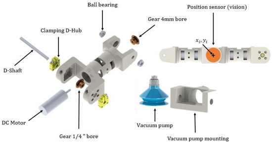
Figure 2.
Elements of each link in the WBRD.
Table 1 describes the dimensions of the angles.

Table 1.
Angular range of the WBRD.
Each link was designed with a scale of yielding a total length of cm in the zero position and a total height of cm including the pumps (Figure 3).
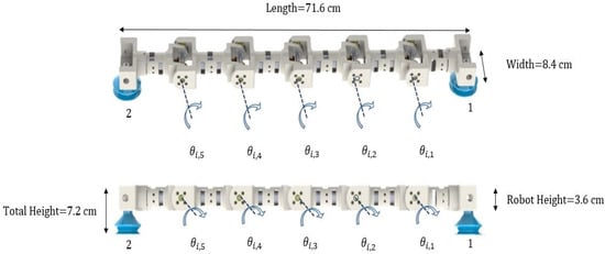
Figure 3.
Dimensions of the WBRD.
3. Problem Definition
The WBRD displacement is represented as an alternated extension–contraction sequences (Figure 4). This simplified representation of the WBRD displacement can be described as a hybrid device alternating the movement of two multi-articulated (5 DOF) manipulators.

Figure 4.
Alternative representation of a gait cycle for the WBRD; (a) The rear pump is on and a first robot manipulator structure is adopted; (b) The reference trajectories force the robot to expand almost to reach a 0 degrees configuration; (c) The pumps switch and the second robot manipulator configuration is adopted, the reference trajectories for the movement of the robot until a desired position; (d) A second switching in the gait cycle is performed to complete the walking path emulating the real inchworm.
The fixation of the reference frame in the suggested alternate way modifies the description of the WBRD. Indeed, this variation of the reference frame forces two distinct dynamic representations for the WBRD. Such condition provides a challenging scenario for developing automatic controllers which can ensure the tracking of reference trajectories that correspond to a bio-inspired gait cycle. This section aims to formulate the controller design problem within the hybrid systems’ framework.
Let us consider the vector of angular displacements within a fixed part ( equal either a or b of the gait cycle . Now, assume that, during the given part of the gait cycle, the angular displacements must track the corresponding reference angles . Then, enforcing the gait cycle for the WBRD can be represented as an stabilization problem for the tracking error , defined as within each continuous domain of .
This problem statement obligates to consider the WBRD dynamics changes only if the vector of tracking errors for all the articulations has attained a sufficiently small value (defined by the user), namely . Therefore, the triggering signal which enforces the dynamics changing can be obtained by measuring the norm of the tracking error within each domain of . Once , then changes from a to b or vice versa.
The problem statement concept given above enforces the fact that the vector of the angular displacements at the WBRD must track the desired reference angles ensuring the tracking errors of all articulations enter the region characterized by at some given finite moment which must be bounded (). Such tracking problem can be described as designing the hybrid controller such that
The maximum allowed switching time is introduced here in order to have a tracking trajectory independent safety condition that can turn off the WBRD if the switching condition is not attained in a reasonable period. Notice that the switching condition introduces a class of a non-constant sampling discrete state which depends on the accomplishment of the condition provided in (1).
This study assumes that only is continuously locally measurable all the time. However, is not available. Therefore, the control design considers an output feedback realization.
4. Hybrid Formulation of the Worm Walking Cycle
The changing dynamics of WBRD can be characterized using a combination of continuous and discrete states. Such representation agrees with the fundamentals of hybrid systems [21]. This formulation to describe the gait evolution of the proposed WBRD is enforced because there is not a strict periodicity which may define the transition between the gait domains (a or b) that is from continuous to continuous (a to b or vice versa) dynamics passing through the discrete state domain.
If the WBRD exerts a regular mono-directional walking gait, the transitions between the continuous stages follows an ordered sequence (a -> b -> a ->...). This sequenced dynamical behavior justifies the application of a class of multi-domain hybrid systems framework considering a predefined order of phases (or domains). Such representation leads to defining a so-called coherent cycle.
Formally, a multi-domain hybrid control system can be described considering a tuple [22,23] , where describes the sequenced cycle of transitions. Consequently, defines a transition vertex connection the continuous domains, represents the subsequent vertex of v during the gait cycle, while corresponds to the transition from the analyzed vertex v to .
Continuous Dynamical Representations. Considering the links masses, their inertia as well as their lengths properties of the WBRD, the equation of motion (EOM) that can be used within a given continuous domain can be determined by the Euler–Lagrange equations (considering that, within a given domain, the WBRD obeys a manipulator representation) [24]. Therefore, assuming that in each fixed domain, the dynamics of the WBRD corresponds to:
Here, , and are the vectors of angular displacements, angular velocities, and the applied torques (operating as the control actuators) respectively for the WBRD.
The drift vector field corresponds to , the state dependent matrix defines the inertia of the WBRD, the matrix defines the Coriolis effects while defines the effect of gravitational force over the WBRD dynamics. The vector function characterizes the control action effect over the WBRD dynamics with .
The uncertain section of the model is gathered in which characterizes the presence of external perturbations and internal modeling uncertainties in the WBRD. Usually, this term aggregates nonlinear behavior such as joint frictions, backslash, and some other elements that are usually complex for modeling.
The function ( is the number of total holonomic restrictions) represents the contact wrenches containing the constraint forces and/or moments. Here, represents the characteristic states occurring during the contact wrenches, and is the corresponding set of control actions which leads to the contact wrenches , which are relevant during the WBRD transition from continuous to continuous domains (floor contact). To enforce the velocity independent (holonomic) constraints, the second order differentiation of the constraints should be set to zero; that is,
The constrained dynamics of the system must be determined using the trajectories of (2) together with (3).
Holonomic Constraints. Given that the WBRD model with coordinates , is the configuration space, the complete dynamics within a domain depends simultaneously on the Lagrangian as well as the contact constraints. All potential contacts of the WBRD with the floor (if not physical obstacles are considered) forces a holonomic constraint, . Considering that is an indexing set of the possible holonomic constraints defined on , then the holonomic constraints of the domain corresponds to constant while the corresponding kinematic constraints corresponds to , is the Jacobian of , i.e., .
The nature of the WBRD justifies that all the states (angular displacements and velocities) are uniformly bounded in time. Therefore, the state is included in the set defined as:
with the i-th component of x, and the corresponding limits and with a small constant real scalar and is either or . Indeed, the set defines the holonomic restrictions for the WDRD structure.
Domains and Guards. A limited number of forces/moments appears if the holonomic constraints are active. These conditions can be represented in the form of component-wise inequalities , is the function containing the parameters of the WBRD. The unilateral constraints in the set complete the admissible configurations for the WBRD via the domain of admissibility :
for . The boundary of each sub-domain are characterized with
A state guard corresponds to a proper subset of the domain boundary, which is determined by an edge condition connected to the transition from to the subsequent domain, . Let us define as an appropriate set of elements taken from (6) which characterize the edge condition. Using such elements, the guard can be characterized as
Discrete Dynamics. Consider the guard as a reset map that connects the system states over the guard to the subsequent domain. Considering the pre-impact states on , the post-impact states of are computed using a reset map by assuming the contact characterized by a perfectly plastic impact (if an impact occurs) [25]. Following the ideas in [26], the states configurations of the WBRD remain invariant during the impact, i.e., ; however, post-impact velocities must satisfy the plastic impact equation:
where defines the impulse function for the forces in the WBRD during the contact with the floor.
Virtual Constraints. Analogously to the described holonomic constraints, virtual constraints (recognized as the tracking errors in the control literature) correspond to the functions that modulates the dynamics the WBRD to track certain reference trajectories. The term virtual arises from the fact that such operative constraints must be enforced via a set of feedback (state or output) control instead of using forced physical restrictions. In equivalence to tracking errors, virtual constraints correspond to . In here, the desired trajectories are proposed accordingly to the technique proposed in [24], where a novel technique to design monotonic and differentiable trajectories over a gait cycle is precisely detailed [27].
Here, one may notice that the goal of the proposed controller is steering to the origin if possible or at least to the zone (indeed, an invariant set) defined in (1) within each continuous domain. In this study, we avoid driving to the invariant set tracking through discrete dynamics. Considering that WBRD must realize movements with the aim of attaining the next switching configurations, the sequence of desired movements and should be calculated considering the distance between objects, the stable configurations for the WBRD, and so on. Notice that the position of the j-th articulation is known in advance assuming that the desired velocity can be estimated by direct differentiation (notice that the design of reference trajectories provides differentiable with continuous derivative flows).
Once the conditions to describe the WBRD have been detailed, it is feasible to propose the controller that can steer the virtual constraints to the origin or at least to the invariant set in (1).
5. Controller Design
5.1. Abstracted Representation of the WBRD
The aim of this research work is developing an output feedback loop controller for a WBRD, which should take into account the hybrid nature of the gait cycle and the state restrictions which define the angular restrictions at each joint. The proposed controller considers then the joints restrictions formed during the standing stage of the WBRD. The dynamics of the WBRD (considering the hybrid nature) is described as follows:
Here, is the vector of angular displacements of the joints considered in the WBRD. The vector is the vector of the angular velocities of all joints. The nature of WBRD structure enforces the existence of restrictions for all components in the state vector that is (4).
The function in (9) represents the drift term that corresponds to internal dynamics of the BIMR:
The function characterizes how the input function affects the robot dynamics. This function is invertible by the nature of the biped robot (formed as class of alternated robotic muti-articulated arm) and satisfies
The bounded function is referred to as the control function, which must take into account the hybrid nature of the WBRD dynamics. By assumption, all the admissible controls belong to the following so-called admissible set:
The term corresponds to admissible class of uncertainties and perturbations affecting the dynamics of WBRD. By assumption, the term satisfies the following restriction:
5.2. H-ADRC Design
Considering the hybrid nature of the WBRD and the state restrictions, there are a few possible controllers that can be used. This study considers the application of a class of output feedback hybrid ADRC which can take into account the state constraints.
The design of the proposed H-ADRC considers the design of an approximation for the uncertain section of the WBRD which is valid within each continuous domain. In this study, let assume that the control free right-hand section of the WBRD dynamics () can be represented as the composition of a nominal model added with a modeling function , which represents those dynamical behaviors that are not modeled, which is .
In this case, this uncertain section added to the external disturbances element can be represented as , where represents the modeling error with describing the nominal model of the WBRD that could be estimated by diverse methods in such a way that the Euler–Lagrange modeling technique is still applicable. In this study, the first option is considered. Consequently, consider the following necessary assumption which must be used in the design of the H-ADRC.
Assumption 1: There exists a matrix of constants for each continuous subsystem such that the function evaluated over the trajectories could be represented as .
In this study, the time-dependent vector (see [28,29] for further details) is
The term is called the modeling error produced by the approximation of by a finite number p of elements in the basis and admits the following bounds by assumption
The so-called nominal model for each continuous domain can be expressed as [30]. In this study, the function can be represented as a chain of integrators of some predefined constant matrices. Thus, the approximation presented above states that must be the solution of an integration operation of an uncertain function plus the approximation error: that is,
Equation (16) can be reorganized in an equivalent differential form:
The vector of initial conditions for is . Now, the problem formulation given can be rephrased as follows: Given an output reference trajectory for the system (9), let us design an output feedback controller that, regardless of the unknown non-modeled dynamics or external disturbances that forces the states x to track asymptotically the desired reference trajectories, with the tracking error restricted to a small neighborhood near the origin and proportional to a power of the uncertainties and perturbations. The first stage in solving this problem is designing an extended state observer to reconstruct the non-measurable part of the state.
5.3. Closed-Loop Dynamics Based on the H-ADRC Structure and Extended State Observer
Let us consider the reference trajectories and that are governed by
where is a continuous function with respect to time which can vary according to the active semi-cycle of the WBRD. The proposed reference trajectories satisfy the following bound for , .
Based on the approximation proposed for and the reference trajectories given in (18), the dynamics of the tracking error are given by
Notice that the bounds for the state x presented as holonomic constraints and the bounds for the reference trajectories provide the following estimation for the bounds of the tracking error in each continuous domain:
The design of the output feedback controller needs to provide an extended state robust state estimator of (9) which in this case satisfies the following hybrid dynamics:
Notice here that , and . The observer gains are defined by and . These gains must be calculated depending on what the active WBRD semi-cycle is.
The dynamics of are associated with an extended state observer connected to:
where .
Let us consider the proposed output-based controller satisfying:
where and are the piece-wise constant gains of the controller which are adjusted in each continuous dynamics.
Let us introduce the extended state vector defined as with . The dynamics of z are described by
with
where , , , ; and .
The stability analysis considers the study over the dynamics of z. This analysis provides the result of the tracking controller, the state estimator, and the reconstruction of the uncertain section in the WBRD dynamics. This methodology yields the satisfaction of the close-loop analysis of the output feedback controller which offers a class of separation-principle for the proposed design. This is an additional theoretical contribution of this study. The following theorem details the main result of this study.
Theorem 1.
Consider the state observer given in (21) and the output feedback controller proposed in (23) with gains adjusted such that all matrices and are Hurwitz for the WBRD dynamics with incomplete information approximated with (17).
If there is a sequence of positive definite matrices and such that positive definite and symmetric solutions and exist for the following matrix inequalities , and with
then the extended state z converges exponentially to the invariant set defined by
with , , are positive and symmetric definite matrices and , are positive definite matrices fulfilling , .
The rate of exponential convergence is given by:
Proof.
The estimation of the adjustment laws for the controller gains uses the concept of Lyapunov stability based on BLF. Formally, the proposed BLF which is used to prove the stability of the origin considers as a class of practical equilibrium point for the movement of the WBRD. In this study, the logarithmic function is used, one of the most common BLFs [31,32]. The suggested BLF function to get the stability analysis in this study is given by
where . Notice then that represents the case a and represents the case b.
The full-time derivative of is
Reorganizing the differential equation (30) yields
The substitution of on the full-time derivative of leads to the following form:
Notice that the term can be handled as follows:
where .
Let us consider the application of the Young inequality, which satisfies:
valid for any ∈ and any N= [33]. Therefore, the following upper bound for is valid:
In equivalent form, accepts the following upper bound:
Introducing the following matrix
The terms including in the time derivative of can be presented as
Noticing that , then
Based on the upper bounds of (13) and the bounds for the modeling error yields to estimating upper norms of and as:
Similarly, the time derivative of (38) can be bounded as
Notice that (40) can be represented as follows:
Taking into account the assumptions that and yielding
If we consider that and , then
Following the ideas given in [20], it is possible to prove that
Consequently, converges asymptotically to the invariant set within a given continuous sub-domain. This is enough to prove the stability within each continuous sub-domain. Now, to prove the stability of the hybrid form, let us consider that the tracking error is already bounded; then, let us propose the discrete analysis for the dynamics of z evaluated on the specific times where the sequential transition from a -> b or vice versa. With the aim of evaluating this stability analysis, one may propose the discrete Lyapunov-like function such as
The discrete analysis of the discrete Lyapunov like function yields
Notice that
With the assumption that the matrix inequality (28) is negative definite, then, is negative and, therefore, the discrete jumps remain negative confirming the local asymptotically stability of the origin for the extended system based on the state z. □
Remark 1.
Notice that the H-ADRC controller can be useful if the proposed control gains can be sufficiently adequate such that . This fact can be guaranteed a priori if a formal optimization of the size for the invariant set proposed in the statement of Theorem 1. The solution of this aspect is outside the scope of this study. However, we assume that the condition described in this remark is fulfilled.
Remark 2.
Notice that adjusting the gains in adaptive form could reduce the large amplitude oscillations along the transient period of the tracking trajectory process. The adaptive adjustment of the gains satisfies:
with . This result can be obtained directly with a similar stability analysis to the one introduced in Theorem 1. The main change is introducing a modified Lyapunov like function satisfying
where and refers to the trace operator. A similar study analysis yields the design of the adaptive gains which can presumably reduce the oscillating transitions.
Remark 3.
The result attained above requires the design of the extended state observer (21), which must provide efficient approximation of the angular velocities of all the articulations. Such condition implies complex instrument requirements for the BIMR. Such condition enforces that the estimation error must converge faster to the corresponding invariant set than the tracking controller does. A possible alternative is using some variant of robust time differentiator which can produce the estimation of the required angular velocities. The so-called super-twisting algorithm can provide such solution, but the close loop stability analysis requires some further work. The reader is referred to the studies given in [34] for more details.
Remark 4.
The application presented in this manuscript needs to solve six different matrix inequalities offline. All of them are Riccati equations and their solutions are quite regular in control theory. Indeed, there exist numerical solvers that can help to find the solution of these inequalities. The requirements to find the solution of a Riccati equation (in general form) given by
are
- The matrix A is Hurwitz, as a consequence:
- The pair is controllable.
- The pair is observable.
Notice that the stability of matrix A in our case is related with the gain matrices and that can be selected in such a way and are Hurwitz.
6. Implementation Issues
The proposed H-ADRC controller requires several technical aspects that must be considered before it can be implemented. This section details the arrangement of all the aspects needed to realize both the numerical and the experimental evaluations.
6.1. Numerical Evaluation
In the simulation system, it is necessary to introduce a force sensing element. The information of the force sensor is used to detect the moment when the corresponding ending section of the WBRD has touched the surface. Notice that such contact must be part of the condition to switch between the subsystems that define the gait scenarios a and b. Including this additional sensor in the condition ensures that the WBRD is completing the semi-cycle in the adequate configuration.
In this study, the numerical simulations used a virtualized representation of the WBRD based on the SimMechanics Toolbox® of Matlab®. The virtual model includes all the articulations and the mechanical representation of vacuum pumps that are going to be used as the electro-mechanical elements to change the reference frame in the hybrid representation of the gait cycle of the WBRD and allowing for evaluating the suggested controller. The mechanical representation of the WBRD was prepared in the Solid-Works® software including all the mobile actions that must be exerted by the WBRD (Figure 5).

Figure 5.
WBRD exported to simMechanics for simulation.
6.2. Experimental Evaluation
The experimental evaluation of the proposed controller was implemented in a polymer-based WBRD. The design of the robot followed the structure proposed in the numerical evaluation. The experimental prototype was constructed using the 3D printing technique using poly-lactic acid (PLA) as building material.
The constructed WBRD used DC motors to realize the mobilization of all joints. A set of gears transmits perpendicular movement to the mechanical structure to reach the desired angular trajectories. Each of the DC actuators was regulated with a DC source to alternate power converter using a pulse width modulation (PWM) methodology.
The numerical realization of the controller used a distributed strategy considering the combination of a processing board (TIVA1294 from Texas Instruments) and a personal computer (Alienware 17S from Dell Computers). The processing board realizes the PWM formulation based on the calculated control action in the personal computer (PC).
The PC realizes an image-based-processing algorithm which calculates the articulation angles using physical markers placed over the WBRD structure (Figure 6). The algorithm is described in Algorithm 1 which is based on the application of simplified morphological image processing methods. The first algorithm is complemented with the calculus of the state estimator (21) and then the output feedback controller proposed in (23) is evaluated according to Algorithm 2. The estimated control action is sent to the processing board via a serial protocol (RS-232).
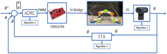
Figure 6.
Implementation control in the WBRD.
The H-ADRC requires including vacuum pumps at the first and the last links of the bio-inspired robot. Each of the pumps is activated once all the angles have attained their reference values. The pump is activated to define the change of the reference framework. The activation action is also evaluated in the algorithm and then sent to the processing board.
| Algorithm 1 Position image recovery | |
| 1: Start | |
| 2: a frame form the camera | ▹ The threshold is selected to find the marker place on the robot joints |
| 3: if and then | ▹ Detect orange markers |
| 4: | |
| 5: else | |
| 6: | |
| 7: end if | |
| 8: if and then | ▹ Detect green markers |
| 9: | |
| 10: else | |
| 11: | |
| 12: end if | |
| 13: imclose(A) | ▹ Morphological closing of the image |
| 14: imopen(B) | ▹ Morphological opening of the image |
| 15: | ▹ Create logical image |
| 16: DetectCentroids(G) | ▹ Function to detect centroids |
| 17: for do | ▹ Calculating the absolute angle with the slope of neighbor centroids |
| 18: | |
| 19: end for | |
| 20: | |
| 21: | |
| 22: for do | ▹ Calculating the relative angle, with respect with the first one |
| 23: | |
| 24: | |
| 25: end for | |
| 26: Return | |
| 27: Start control calculation | ▹ Go to Algorithm 2 |
| Algorithm 2 Control implementation | |
| 1: Start | |
| 2: Obtain the corresponding angles | ▹ From Algorithm 1 |
| 3: Check the switching condition ▹ To see what pump is active and the corresponding system | |
| 4: Implement the extended observer to recover from Equation (17) | ▹ To recover and |
| 5: Implement the control law in (23) for the corresponding system | |
| 6: Evaluate the obtained decoupled controllers to convert into a pulse modulation signal (PWM) | |
| 7: if then | ▹ These values correspond to the high time in the PWM signal |
| 8: | |
| 9: else | |
| 10: | |
| 11: end if | |
| 12: Evaluete the control to determine the movement direction of the actuators | |
| 13: if then | |
| 14: | |
| 15: else | |
| 16: | |
| 17: end if | |
| 18: Send the values through serial comunication (RS-232 protocol) to the TIVA1294 | |
| 19: Activate a PWM with the values of and to be sent to the H bidges | |
| 20: Return to Algorithm 1 to calculate again the current position | |
7. Simulation Results
The proposed output feedback controller was evaluated using a set of numerical evaluations considering the exerting of three completes gait cycles. The corresponding sequences of reference angular movements were calculated using a biomechanical study of a Leptidoptera gonodonta or measuring worm. Once the angles were calculated, the method to produce the reference trajectories was implemented. These reference trajectories were injected into the SimMechanics software.
The numerically simulated model in SimMechanics-Matlab was evaluated considering the real masses (assuming the construction based on PLA material) and dimensions of each mechanical section of the WBRD. This strategy allowed for evaluating the controller as well as tuning the gains of both the estimators and controllers. These gains were used as the initial values in the experimental device.
The angular trajectories measured from the simulated WBRD were compared with the reference trajectories (Figure 7). The shown trajectories correspond to the reference signals, the measured position with the proposed H-ADRC (using the estimated velocities from the state estimator), and the state feedback form. The comparison of all trajectories confirms that the H-ADRC controller provides an equally faster convergence than other controllers, but it has less oscillations during the transient period. Such characteristic is a consequence of the additional compensation provided by the extended state observer that can actively compensate the effect of external perturbations and internal modeling imprecision. The comparison with a classical PID controller confirms such additional benefit of introducing the augmented compensation aggregated in the H-ADRC form. In addition, the proposed controller tracks the reference with smaller deviations than all other controllers considered for comparison. Notice also that these trajectories confirm the presence of high-frequency oscillations at the beginning of the tracking period (first three seconds). Although these oscillations may be undesired for the WBRD movements, the tracking exerted after the oscillations period justifies the introduction of H-ADRC based compensation due to its robustness against matched perturbations.
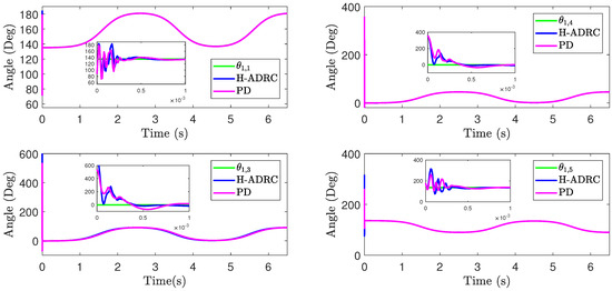
Figure 7.
Comparison of reference trajectories with controlled states implementing either the PD and the proposed H-ADRC controllers.
Figure 8 shows (in logarithmic scale) the control associated energy enforced by the state feedback (marked with PD) and the H-ADRC controllers. This comparison considers that both controllers solve the tracking with the same convergence quality. The application of the compensated control form consumes smaller amounts of energy and augments the working life of the DC motors’ actuators. These controllers were chosen for this comparison because they provided the best trajectory tracking among the evaluated controllers.
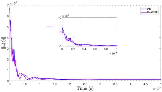
Figure 8.
Euclidean norm of the control energy used with each control algorithm.
Figure 9 details the comparison of the Euclidean norms of the tracking errors obtained with the application of the same evaluated controllers that were presented in Figure 8. This figure highlights the rate of convergence and the ultimately bounded zone for the tracking errors. This figure is also presented in logarithm scale for the purpose of better detecting the differences among the proposed controllers. In both cases, the H-ADRC forces a faster convergence and smaller oscillations amplitude in steady-state for the controlled trajectories.
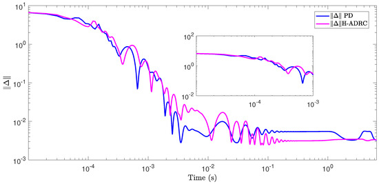
Figure 9.
Euclidean norm of the tracking error for each control technique used in simulation.
Figure 10 demonstrates a sequence of image captures obtained from the simulated evaluation of the H-ADRC application over the WBRD. This sequence highlights the sequence of movements exerted by the entire simulated WBRD associated with the sequence of articular movements enforced by the distributed form of the proposed controllers. The sequence also demonstrates the benefits of introducing the simulated SimMechanics model because it allows for getting an efficient gains adjustment which yields to satisfying the complete gait sequence. Moreover, the hybrid analysis of the controller is confirmed with the efficient tracking of the reference angular positions in both scenarios a and b.
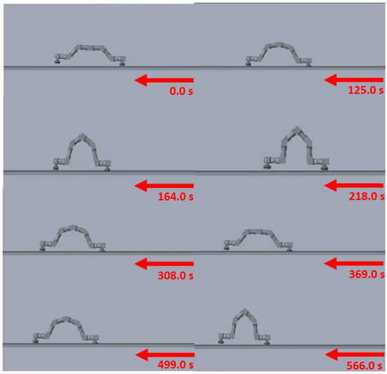
Figure 10.
Sequence of movements of the gait cycle of the WBRD in simulation.
8. Experimental Results
Once the simulated evaluation showed acceptable results measured in terms of the tracking errors and the consumed energy, the control was implemented according to Algorithms 1 and 2. Different controllers were implemented with the aim of evaluating the advantages of the proposed methodology. The H-ADRC controller was compared with the classical state feedback controller using the derivative obtained by means of the extended state observer and an experimental PID form.
Figure 11 shows the comparison of the angular displacements obtained in the experimental results with three different controllers. For the PD controller supplied with the estimated derivative, the vector of the five different proportional gains were selected as and the derivative gains were . The case of the integral part included the same proportional and derivative gains while the integral gains were: . The hardware configuration used to evaluate the proposed controller provided an updating time of the control action of 0.05 s, which was enough to successfully realize the gait cycle by the experimental WBRD.
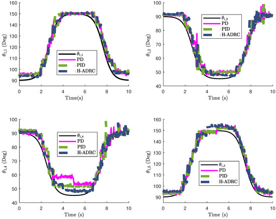
Figure 11.
Comparison of the trajectory tracking task in the WBRD by means of different control techniques.
The comparison of the proposed controllers confirmed that the observed additional compensation of the H-ADRC improves the tracking efficiency for all the articulations. Moreover, the oscillations of the measured angular are reduced during the transient period. In addition, one may notice that state feedback provides the worst tracking performance among the evaluated controllers. This result was also true for all the trajectories in the constructed WBRD.
The comparison of the controllers’ performances was realized through the calculus of the norm of the tracking errors (Figure 12a). This comparison proves that the tracking error is smaller if the evaluated controller was the H-ADRC in comparison with the other two controllers (state feedback and PID). Notice that the PID form provides a comparable tracking quality to the H-ADRC. Notice that a fair comparison between the evaluated controllers cannot include the norm of the tracking error only, but it must include the energy associated with the controller. Here, one may notice that H-ADRC uses larger energy (measured in terms of the norm of the control action) than the other two controllers (Figure 12b). This increment is actually not significant (), and it occurs only during the of the evaluated period corresponding to the gait cycle.

Figure 12.
Performance index for each control technique: (a) comparison of the Euclidean norm of the tracking error; (b) energy used by each controller represented by the evolution of the integral of the square control action u.
Figure 13 provides a sequence of photographs corresponding to the experimental evaluation of the H-ADRC controller over the constructed WBRD. These photos reveal a sequence of the BIMR positions if the controller BIMR regulates the DC motor actuators yielding a coordinated articular movements. The sequence confirms the effects of the additional compensation integrated in the H-ADRC. Additionally, the sequence confirms the performance of the alternated activation of the vacuum pumps according to the realization of the gait semi-cycle in either scenario a or b.
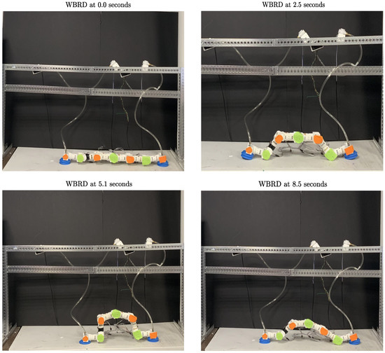
Figure 13.
Experimental gait sequence.
Experimentally, the hybrid controller provides the efficient tracking of the reference angular positions in both scenarios a and b, despite the model of the WBRD not having been used at all in the experimental sequences.
Figure 14 is intended to highlight the sequence realized by pumps that remain attached to the floor after the proposed controller drives the trajectories toward the references (red arrows for the attached and blue arrows for the released pumps). This strategy succeeded in keeping the angular velocities bounded at each joint in the bioinspired robot. In addition, the reference trajectories for the controller were proposed to keep the distal section of the WBRD closer to the floor. In addition, the absolute values of their time derivatives are small enough to limit the possibility of having fast variations of the controlled angular position at each join, which also contributes to reducing high frequency oscillation of the tracking error. All of these strategies together restricted the possibility of the discontinuous movements’ effect on the proposed WBRD.
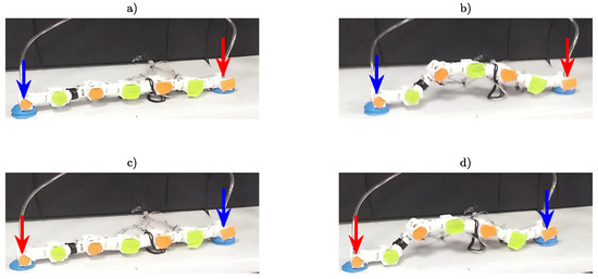
Figure 14.
Reference framework switching: (a) second vacuum pump activated (red arrow) in zero position; (b) second vacuum pump activated during gait cycle; (c) first vacuum pump activated in zero position; (d) first vacuum pump activated during gait cycle.
Remark 5.
The magnitude of the control signal depends on the initial conditions of the position and velocities of the suggested mobile robot links. Moreover, the magnitude of the control is a trade-off between the convergence time, as well as the accuracy on the tracking error. This problem can be solved by an adaptive version of the controller in order to reduce the control magnitude as the tracking error approaches the origin. In addition, the energy is necessary to fulfill the restrictions imposed by the Barrier function. In the case of the experimental results, the control signal is restricted according to the signal that is sent to the robotic device, which means that a pulse Width modulated (PWM) signal is implemented in the device. The maximum value for the control output is with N the number of bits used for implementing PWM signal. Under this condition, the CD motor is moving as its maximum speed, which is always bounded.
9. Conclusions
The proposed controller exhibited an acceptable performance even in the presence of parametric uncertainties and noisy measurements. The hybrid structure allows for dealing with the WRBD represented by two link robot manipulators alternating between their first and last links as a reference for its working space. This result constitutes one of the first ADRC approaches dealing at the same time with hybrid systems with restricted variables. A barrier technique imposed angular restrictions in the robotic device avoiding any damage to its physical structure. Moreover, the H-ADRC controller reduces the steady state error compared with classical output feedback structures like state-feedback (PD form) and extended state state feedback (PID structure).
Author Contributions
Conceptualization: I.S., D.C.-O. and I.C.; Methodology: V.L.-O. and A.G.; Software: A.G. and M.M.-S.; Validation: V.L.-O., A.G. and M.M.-S.; Formal analysis, I.S. and D.C.-O.; Investigation: V.L.-O. and D.C.-O.; Resources: I.S. and I.C.; Data curation: V.L.-O. and M.M.-S.; Writing—original draft preparation: V.L.-O. and I.S.; writing—review and editing: I.S. and I.C.; supervision: I.C.; project administration: I.S., D.C.-O. and I.C.; Funding acquisition: I.S., D.C.-O. and I.C. All authors have read and agreed to the published version of the manuscript.
Acknowledgments
The authors acknowledge the support and funding offered by the National Polytechnique Institute via the Grants labeled SIP-2019-5253, SIP-2019-5253 and SIP-2019-6849.
Conflicts of Interest
Authors declare not any personal interest that may be perceived as inappropriately influencing the representation or interpretation of reported research results.
References
- Hwang, J.; Jeong, Y.; Park, J.M.; Lee, K.H.; Hong, J.W.; Choi, J. Biomimetics: Forecasting the future of science, engineering, and medicine. Int. J. Nanomed. 2015, 10, 5701. [Google Scholar] [CrossRef]
- Hyun, D.J.; Seok, S.; Lee, J.; Kim, S. High speed trot-running: Implementation of a hierarchical controller using proprioceptive impedance control on the MIT Cheetah. Int. J. Robot. Res. 2014, 33, 1417–1445. [Google Scholar] [CrossRef]
- Wiguna, T.; Heo, S.; Park, H.; Seo Goo, N. Design and Experimental Parameteric Study of a Fish Robot Actuated by Piezoelectric Actuators. J. Intell. Mater. Syst. Struct. 2009, 20, 751–758. [Google Scholar] [CrossRef]
- Kim, S.; Spenko, M.; Trujillo, S.; Heyneman, B.; Santos, D.; Cutkosky, M.R. Smooth Vertical Surface Climbing With Directional Adhesion. IEEE Trans. Robot. 2008, 24, 65–74. [Google Scholar] [CrossRef]
- Seok, S.; Onal, C.D.; Cho, K.J.; Wood, R.J.; Rus, D.; Kim, S. Meshworm: A peristaltic soft robot with antagonistic nickel titanium coil actuators. IEEE/ASME Trans. Mechatron. 2013, 18, 1485–1497. [Google Scholar] [CrossRef]
- Umedachi, T.; Vikas, V.; Trimmer, B.A. Softworms: The design and control of non-pneumatic, 3D-printed, deformable robots. Bioinspiration Biomim. 2016, 11, 025001. [Google Scholar] [CrossRef]
- Qiao, J.; Shang, J.; Goldenberg, A. Development of Inchworm In-Pipe Robot Based on Self-Locking Mechanism. IEEE/ASME Trans. Mechatron. 2013, 18, 799–806. [Google Scholar] [CrossRef]
- Plaut, R.H. Mathematical model of inchworm locomotion. Int. J. Non-Linear Mech. 2015, 76, 56–63. [Google Scholar] [CrossRef]
- Lee, D.; Joe, S.; Choi, J.; Lee, B.I.; Kim, B. An elastic caterpillar-based self-propelled robotic colonoscope with high safety and mobility. Mechatronics 2016, 39, 54–62. [Google Scholar] [CrossRef]
- Jung, G.P.; Koh, J.S.; Cho, K.J. Underactuated adaptive gripper using flexural buckling. IEEE Trans. Robot. 2013, 29, 1396–1407. [Google Scholar] [CrossRef]
- Saab, W.; Kumar, A.; Ben-Tzvi, P. Design and Analysis of a Miniature Modular Inchworm Robot. In Proceedings of the ASME 2016 International Design Engineering Technical Conferences and Computers and Information in Engineering Conference, Charlotte, NC, USA, 21–24 August 2016; p. V05AT07A060–V05AT07A060. [Google Scholar]
- Moreland, S.; Skonieczny, K.; Wettergreen, D.; Asnani, V.; Creager, C.; Oravec, H. Inching locomotion for planetary rover mobility. In Proceedings of the 2011 Aerospace Conference, Big Sky, MT, USA, 5–12 March 2011; pp. 1–6. [Google Scholar] [CrossRef]
- Tang, D.; Zhang, W.; Jiang, S.; Shen, Y.; Chen, H. Development of an Inchworm Boring Robot (IBR) for planetary subsurface exploration. In Proceedings of the 2015 IEEE International Conference on Robotics and Biomimetics (ROBIO), Zhuhai, China, 6–9 December 2015; pp. 2109–2114. [Google Scholar] [CrossRef]
- Guan, Y.; Jiang, L.; Zhu, H.; Zhou, X.; Cai, C.; Wu, W.; Li, Z.; Zhang, H.; Zhang, X. Climbot: A modular bio-inspired biped climbing robot. In Proceedings of the 2011 IEEE/RSJ International Conference on Intelligent Robots and Systems, San Francisco, CA, USA, 25–30 September 2011; pp. 1473–1478. [Google Scholar] [CrossRef]
- Rahmani, M.; Ghanbari, A.; Ettefagh, M.M. Robust adaptive control of a bio-inspired robot manipulator using bat algorithm. Expert Syst. Appl. 2016, 56, 164–176. [Google Scholar] [CrossRef]
- Ayala, H.V.H.; dos Santos Coelho, L. Tuning of PID controller based on a multiobjective genetic algorithm applied to a robotic manipulator. Expert Syst. Appl. 2012, 39, 8968–8974. [Google Scholar] [CrossRef]
- Kolathaya, S.; Ames, A.D. Parameter to state stability of control Lyapunov functions for hybrid system models of 6 robots. Nonlinear Anal. Hybrid Syst. 2017, 25, 174–191. [Google Scholar] [CrossRef]
- Xie, H.; Song, K.; He, Y. A hybrid disturbance rejection control solution for variable valve timing system of gasoline engines. ISA Trans. 2014, 53, 889–898. [Google Scholar] [CrossRef] [PubMed]
- Sira-Ramírez, H.; Luviano-Juárez, A.; Ramírez-Neria, M.; Zurita-Bustamante, E.W. Chapter 2—Generalities of ADRC. In Active Disturbance Rejection Control of Dynamic Systems; Sira-Ramírez, H., Luviano-Juárez, A., Ramírez-Neria, M., Zurita-Bustamante, E.W., Eds.; Butterworth-Heinemann: Oxford, UK, 2017; pp. 13–50. [Google Scholar] [CrossRef]
- Tee, K.P.; Ge, S.S.; Tay, E.H. Barrier Lyapunov Functions for the control of output-constrained nonlinear systems. Automatica 2009, 45, 918–927. [Google Scholar] [CrossRef]
- Schaft, A.; Schumacher, H. An Introduction to Hybrid Dynamical Systems; Springer: London, UK, 2000. [Google Scholar]
- Park, J.H.; Chung, H. Hybrid control for biped robots using impedance control and computed-torque control. In Proceedings of the 1999 IEEE International Conference on Robotics and Automation, Detroit, MI, USA, 10–15 May 1999; Volume 2, pp. 1365–1370. [Google Scholar]
- Martin, A.E.; Post, D.C.; Schmiedeler, J.P. Design and experimental implementation of a hybrid zero dynamics-based controller for planar bipeds with curved feet. Int. J. Robot. Res. 2014, 33, 988–1005. [Google Scholar] [CrossRef]
- Cruz, D.; Luviano-Juárez, A.; Chairez, I. Output sliding mode controller to regulate the gait of Gecko-inspired robot. In Proceedings of the Memorias del XVI Congreso Latinoamericano de Control Automático, Cancún Quintana Roo, México, 14–17 October 2014. [Google Scholar]
- Bullo, F.; Zefran, M. Modeling and controllability for a class of hybrid mechanical systems. IEEE Trans. Robot. Autom. 2002, 18, 563–573. [Google Scholar] [CrossRef]
- Posa, M.; Tedrake, R. Direct trajectory optimization of rigid body dynamical systems through contact. In Algorithmic Foundations of Robotics X; Springer: Berlin, Germany, 2013; pp. 527–542. [Google Scholar]
- Merchant, R.; Cruz-Ortiz, D.; Ballesteros-Escamilla, M.; Chairez, I. Integrated wearable and self-carrying active upper limb orthosis. Proc. Inst. Mech. Eng. H J. Eng. Med. 2018, 232, 172–184. [Google Scholar] [CrossRef]
- Sira-Ramírez, H.; López-Uribe, C.; Velasco-Villa, M. Linear Observer-Based Active Disturbance Rejection Control of the Omnidirectional Mobile Robot. Asian J. Control 2013, 15, 51–63. [Google Scholar] [CrossRef]
- Morales, R.; Sira-Ramírez, H.; Feliu, V. Adaptive control based on fast online algebraic identification and GPI control for magnetic levitation systems with time-varying input gain. Int. J. Control 2014, 87, 1604–1621. [Google Scholar] [CrossRef]
- Sira-Ramirez, H.; Nuñez, C.; Visairo, N. Robust Sigma - Delta Generalised Proportional Integral observer based control of a buck converter with uncertain loads. Int. J. Control 2010, 83, 1631–1640. [Google Scholar] [CrossRef]
- Liu, Y.J.; Tong, S. Barrier Lyapunov functions-based adaptive control for a class of nonlinear pure-feedback systems with full state constraints. Automatica 2016, 64, 70–75. [Google Scholar] [CrossRef]
- Yu, X.; Wang, T.; Qiu, J.; Gao, H. Barrier Lyapunov Function-Based Adaptive Fault-Tolerant Control for a Class of Strict-Feedback Stochastic Nonlinear Systems. IEEE Trans. Cybern. 2019. [Google Scholar] [CrossRef]
- Poznyak, A. Advanced Mathematical Tools for Control Engineers: Volume 1: Deterministic Systems; Elsevier: Amsterdam, The Netherlands, 2010. [Google Scholar]
- Salgado, I.; Cruz-Ortiz, D.; Camacho, O.; Chairez, I. Output feedback control of a skid-steered mobile robot based on the super-twisting algorithm. Control Eng. Pract. 2017, 58, 193–203. [Google Scholar] [CrossRef]


© 2020 by the authors. Licensee MDPI, Basel, Switzerland. This article is an open access article distributed under the terms and conditions of the Creative Commons Attribution (CC BY) license (http://creativecommons.org/licenses/by/4.0/).