1. Introduction
The pioneering work of [
1,
2] on population biology is the threshold created in today’s explosion of the field of population biology. The area has become vast, enriching the field of epidemiology and medicine. The framework of the Lotka–Volterra model is the two differential equations with a simple proportionality between the prey consumption and predation production. The proportional elements have been many functions and the modeling has become more realistic. The proportional functions are the functional response or trophic interaction functions. The Holling type I II III [
3] are old to represent a predator–prey system. The prey dependence [
4] trophic interactions in the population model have reigned for long time, even today [
5]. Such a category of population models cannot produce the situations of biological control. If the trophic function depends on the single variable
(
N, the prey,
P, the predator), then the essential properties of predator dependence are rendered, called ratio-dependence [
4]. The work on this ratio-dependence model has mainly focused on continuous models. Such a model only gives some bifurcation and limit cycle as the population evolution. But the discrete time predator–prey models have richer dynamics than the continuous counterpart. The discrete model can explain the basin of attraction, fractal dimension and the chaotic behavior of an attractor and the sensitive dependence of initial conditions. Danca demonstrated that the discrete-time predator–prey model with Holling type I functional response exhibits a chaotic behavior [
6]. More realistic results are obtained in the works of [
7,
8]. The discrete time ratio-dependent predator–prey explains the chaotic dynamics of the model system. The study sheds more light on the complex dynamical behavior. In this chapter, we investigated the stability behavior and different features of a discrete type ratio-dependent predator–prey system.
In this paper, we investigated the stability behavior and different features of a discrete type ratio-dependent predator–prey system. In
Section 3, we studied the local stability analysis by using Jury’s conditions. In
Section 4, we performed and presented diffusion dynamics.
Section 5 deals with noise impact on the stochastic system. In
Section 6, we presented computer simulations with notable significances as maximal Lyapunov exponents responsible for chaos of the system and existence of orbit due to sensitivity. In
Section 7, the entire compilation of analysis with results is presented as concluding remarks.
2. The Discrete-Time Model Equations
We begin with the continuous-time predator–prey system. In most predator–prey systems, the predator is to search for food and also compete for food, and the more realistic functional response is a function which is dependent on both prey and predator densities. The Michaelis-Menten type functional response introduced by [
4] is given by
where
N,
P are, respectively, the prey and predator densities,
a is the maximum prey consumption rate, and
h is the predator handling time. This ratio-dependent functional response is strongly supported by numerous fields, laboratory experiments, and ecological literatures [
9,
10,
11,
12]. With this functional response, the general type ratio-dependent predator–prey system due to [
9] is
Here,
is the prey growth rate in the absence of predator,
d is the death rate of the predator in absence of prey. Here, we consider the logistic growth rate of the prey given by
So, the general ratio-dependent predator–prey model becomes
where
r,
K are, respectively, the intrinsic growth rate and environmental carrying capacity of the prey in the absence of predator.
The number of independent parameters can be reduced by using the dimensionless quantities for prey
N, predator
P and time
t as follows:
,
, and
. Then, the system becomes
where
,
, and
. It is available in any standard literature. Thus,
is the consumption ability,
is the death rate of the predator, and
is the predator growing ability.
The model system (
5) is the standard ratio-dependent predator–prey model studied by many authors [
5]. In this work, we consider the discrete-time predator–prey model analogous to its continuous counterpart (
5). In the continuous time model (
5), we replace the derivatives with the divided differences
and then, taking
, the above system of equations reduces to
where
,
. In this study, the system of Equation (
7) represents the main equations of interest. Thus, the continuous system which represents a flow of two predator and prey is now a 2-dimensional map of two species from the discrete time
n to
. If this map is denoted by
T, then
governed by the set of Equation (
7). This map will determine the population evolution from the initial state
to a state
, so that
. This evolution will move through different complex dynamical phenomena.
3. Steady State Analysis
We studied the stability behavior of the two-dimensional map governed by the set in Equation (
7). The fixed points of the map are given by
. So, we have the following three fixed points: (i) Extinction of both predator and prey population:
, (ii) extinction of predator population:
, and (iii) the coexistence of both the population predator and prey:
, where
and
.
The first two fixed points, and , are always biologically feasible. The feasibility of the fixed point demands with .
To study the stability behavior of the system near the fixed points, we linearize the model equations about the fixed points. If
be the small perturbations corresponding to the fixed point
, then
and
. The linearized system of the above system of equations is
where
.
We seek a solution of the form
to Equation (
8), where
A and
B are arbitrary constants. So, the characteristic equation will determine the value of
which, in turn, will help in giving the dynamical behavior of the fixed point. The characteristic equation of the system of Equation (
8) is
where
, and
. Let
and
be characteristic roots of Equation (
10) and also suppose that
. Then, the equilibrium point
is
- (i)
stable if , , that is, if and .
- (ii)
unstable if , , that is, if and .
- (iii)
saddle if , (or , ), that is, if . We now analyze the stability behavior at several fixed points.
3.1. Dynamical Behavior of
As the functional response is not defined at
, the fixed point
is most complicated for the ratio-dependent model system. We choose a neighboring point
in the first quadrant corresponding to the fixed point
. Then, the Jacobian matrix
is given by
Then, the linearized system is
The characteristic equation corresponding to the fixed point
is
Using the above criteria for dynamical behavior we list the conditions as follows: the fixed point is
- (i)
stable if (a) and , or, (b) and ,
- (ii)
unstable if (a) and , or, (b) and ,
- (iii)
saddle point if .
3.2. Dynamical Behavior of
The Jacobian matrix of system (
8) at
is
The corresponding linearized system is given by
So, is stable if or a saddle point if does not belong to .
3.3. Dynamical Behavior of
The Jacobian matrix of System (
8) corresponding to
is
The linearized system corresponding to the interior equilibrium point is
The characteristic equation of the above system is
From the characteristic Equation (
15), we can conclude that the fixed point
is
- (i)
stable if
,
, and
lie in the parametric space
If mathematical observations drawn here interpret the biological conclusion as if the consumption ability is less than the predator growing ability, then the model system attains its stability, and its dynamics explored more clearly to pick some interesting remarks:
- (ii)
unstable if
,
and
lie in the parametric space
where
.
If mathematical observations drawn here interpret the biological conclusion as if the consumption ability is greater than the predator growing ability, then the model system reaches unstable and, further, there is a chance to attain its stability by additional driven forces or parameters with an appropriate controller/adapter to exhibit its dynamics as effectively and interestingly, which is an advanced wide study.
- (iii)
saddle if which is a contradiction for the existence of .
If mathematical observations drawn here interpret the biological conclusion as if the difference between the predator growing ability and its death rate is greater than the ratio of predator growing ability to consumption ability, then the model system reaches saddle point, which is an uncertainty where it is neither stable nor unstable and no further dynamics are exhibited by the model system.
These are the conditions that the system exhibits different dynamical behavior.
4. Diffusive Structure and Its Dynamic Forces
In this segment, we deliberated the exceptional influences of transmission of the ideal structure of prey predator systems in environmental science, modeled by diffusion equations. Although the dispersal system is a relatively simple model for the raid of prey species by predators in a spatial domain, the solutions exhibit an extensive spectrum of ecologically pertinent behavior. Spatiotemporal dynamics includes chaos and target patterns [
13,
14,
15]. The study of such spatiotemporal dynamics is an intensive area of research, and there are still many unanswered questions concerning these solution types [
15,
16,
17]. Constructing a simple structure, which consists of prey-predator system with constant harvesting rates and temporal affects, in this segment, we next examine the steadiness of the proposed model under the external dynamical forces as our aim in the next segment. The actual dynamics of the species spread is a result of the interplay between diffusion and deterministic factors. To study the effect of diffusion of ecological population on the model system, let us consider the diffusive equation system as
where
,
u is a space variable, and
;
for
The trivial fluctuation edge conditions are specified by
Now, let us consider the ideal (
16) and (
17) underneath trivial fluctuations edge ailments. To analyze the role of transmission on this ideal, we deliberate the linear ideal of the structure (
16) and (
17) about the interior steady state
as given by
by putting
;
and assuming the solutions of Equations (
16) and (
17) in the form
where
p is the wave numeral of perturbation,
is the frequency numeral, and
are the amplitudes. The characteristic equation of (
16) and (
17) using (
20) is
where
;
.
Now, our main aim is to find the ailments for diffusive unsteadiness of model system (
16) and (
17), for this, rewrite
as
, where
.
The system (
16) and (
17) is unstable if one of the above roots of the Equation (
21) is optimistic. An essential ailment for a solution to be optimistic is that
, which implies that
Since the wave number
p is real number, then the above statement is achievable, if
, which is always achieved, because by nature
is real number. The sufficient condition for optimitive of one of the solutions of the Equation (
22) is
. Since
is an expression in
where
p is the wave number, non-zero positive quantity, the sufficient condition reduces to
where
. Thus, the diffusion of the prey-predator populations drive the ecological system into unstable oscillation when (
22) and (
23) are satisfied. According to Routh–Hurwitz principle, the essential and adequate ailments for local steadiness of
are
;
Theorem 1. The point is locally asymptotically stable in the attendance of transmission if and .
The above statement is followed immediately by R–H criteria.
Theorem 2. (i) The system in the absence of spatiotemporal attributes at the inner steady state attains steadiness, then the corresponding uniform steady state of the model system (16) and (17) in the presence of spatiotemporal attributes also attains steadiness. (ii) If the inner steady state of the non-spatial heterogeneity system is unstable, then the respective steady state of the spatiotemporal model system (16) and (17) under initial and boundary settings and attain steadiness by increasing or decreasing the spatiotemporal attributes suitably. Proof. Let us define the function
, where
is defined in Stability analysis section. Differentiating
w.r.t.
t along the solutions of the diffusive model (
16) and (
17), we get,
where
Using the analysis in [
14], we get
From (
24) and (
25), it is observed that if
, then
is negative. If
, then it is clearly showing if there is an increase in the spatiotemporal attributes
and
adequately huge numeral,
as
. Henceforth are the succeeding portion of the theorem grasps. □
5. Impact of Environmental Noise on the Model System
Ecological systems are characteristically forced by a number of drivers such as climate and natural disturbances that are not constant in time but fluctuate. With the exception of processes dominated by deterministic oscillations, a significant part of environmental variability is random because of the uncertainty intrinsic in weather patterns, climate fluctuations, and episodic disturbances like earth quakes, landslides, fires, insect outbreaks, etc. The recurrence of random drivers in bio-geophysical processes motivates the study of how a stochastic environment may affect and determine the dynamics of natural systems. We now begin introducing noise on the proposed model (
5) to analyze the role of random environmental fluctuations on stability. The random fluctuations make the parameters of the model to oscillate about their average values. We consider such randomness to the model (
5) by incorporating additive white noises. The white noise perturbation included will change any parameter
of the model as
, where
is the amplitude of the noise and
is a Gaussian white noise process at time
t, but the deterministic and stochastic models have same equilibria which will also now fluctuate about their mean states. By considering the randomly fluctuating driving forces in the form of additive noise to the model (
5), we get the following stochastic model
where
are real constants, and
is a two dimensional Gaussian white noise process agreeable
;
, where
is the Kronecker symbol;
is the delta-Dirac function.
In this analysis, we focus on the dynamics of the model (
26) and (
27) at the interior equilibrium point
only according to the method introduced by Nisbet and Gurney [
18] and Carletti [
19]. Let
and by considering only the consequence of linear stochastic perturbations.
Hence, the model (
26) and (
27) reduces to the following linear system
Taking the Fourier transform of (
28) and (
29), we get,
The matrix form of (
30) and (
31) is
where
;
;
;
Hence, the solution of (
32) is given by
, where
The solution components of (
34) are given by
The spectrum of are given by .
Hence, the intensities of fluctuations in the variable
are given by
where
;
;
.
If we consider the noise effect on any one of the species, which is with either or then we have ; if ; ; if .
The population variances point out the stability of population for smaller values of mean square fluctuations, while the larger values of population variances indicate the instability of the populations.
6. Computer Simulations
We want to verify the analytical results obtained in the previous section for the stability of System (
7). We numerically calculate the maximal Lyapunov exponent and show the chaotic behavior of the system for the presence of the positive Lyapunov exponent of the system. And also we want to analyze the sensitive dependence of the system trajectories on initial conditions.
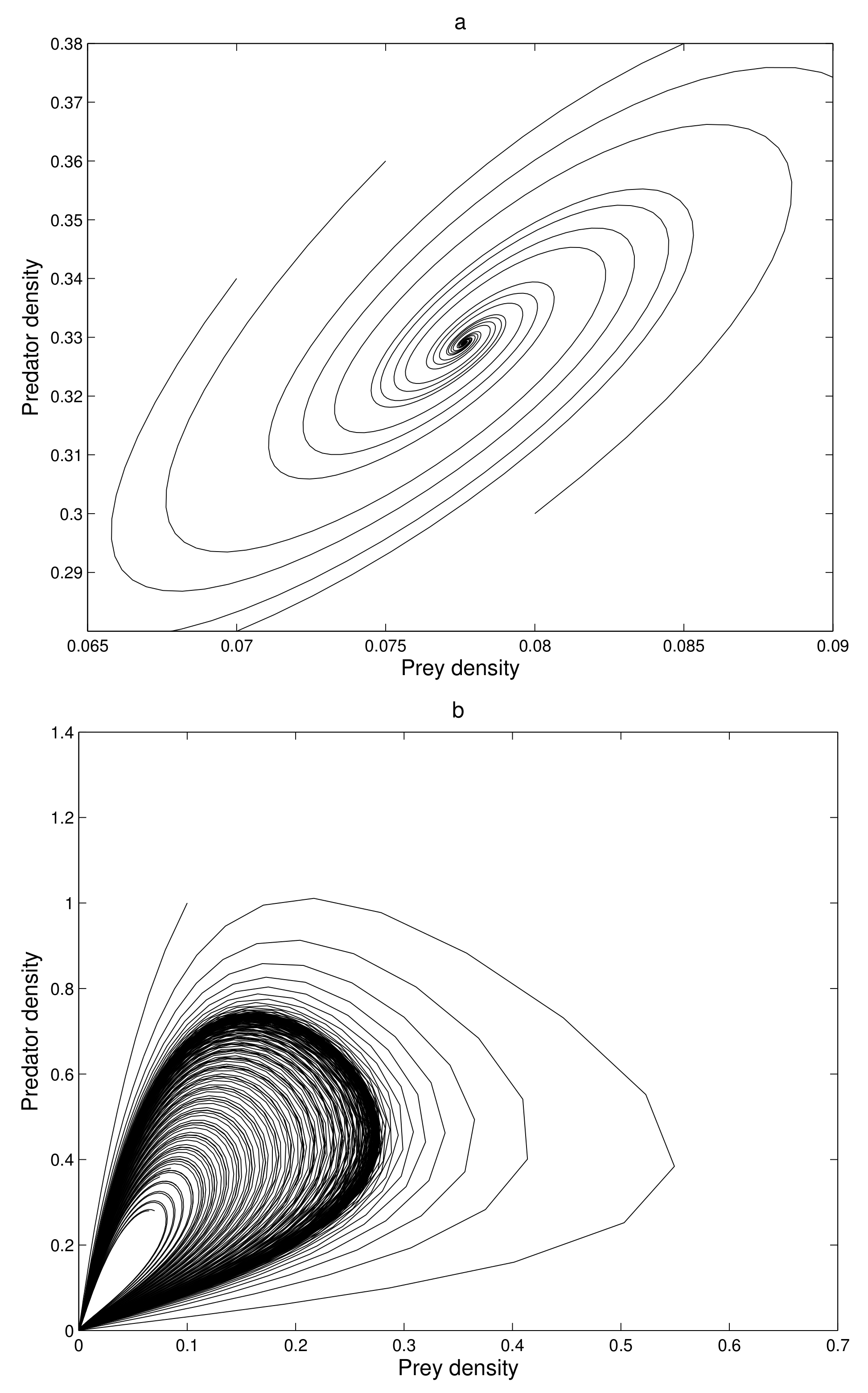
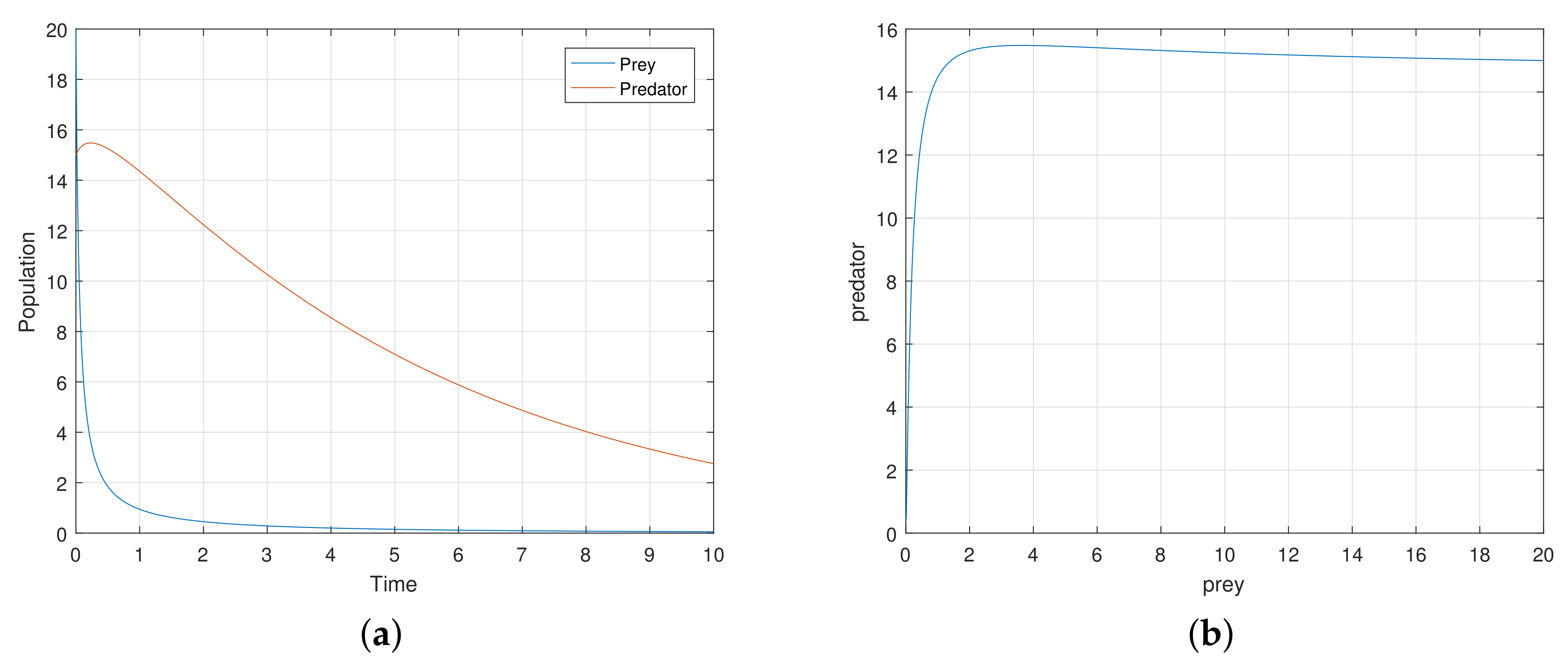
At first, we verify that the system moves to a stable state for a particular values of the parameters. We take the parameters value
,
,
satisfying the stability criteria listed in the previous section. Then, the 2-dimensional map (
7) exhibits a stable movement towards the endemic equilibrium point
(see
Figure 1a).
The eigenvalues of the system are complex numbers for the same parameter value, and its absolute value is
. This fact also suggests that the system is stable about the endemic equilibrium point
. At this stage, we want to state that, for the adjoining
Figure 1a, the phase-portraits are obtained from several initial states. All the initial populations converge to a single state (point)
, the attractor. The basin of attractor is the set of all initial points which converge to
. Here, the basin of attraction is
, and the corresponding attractor is
.
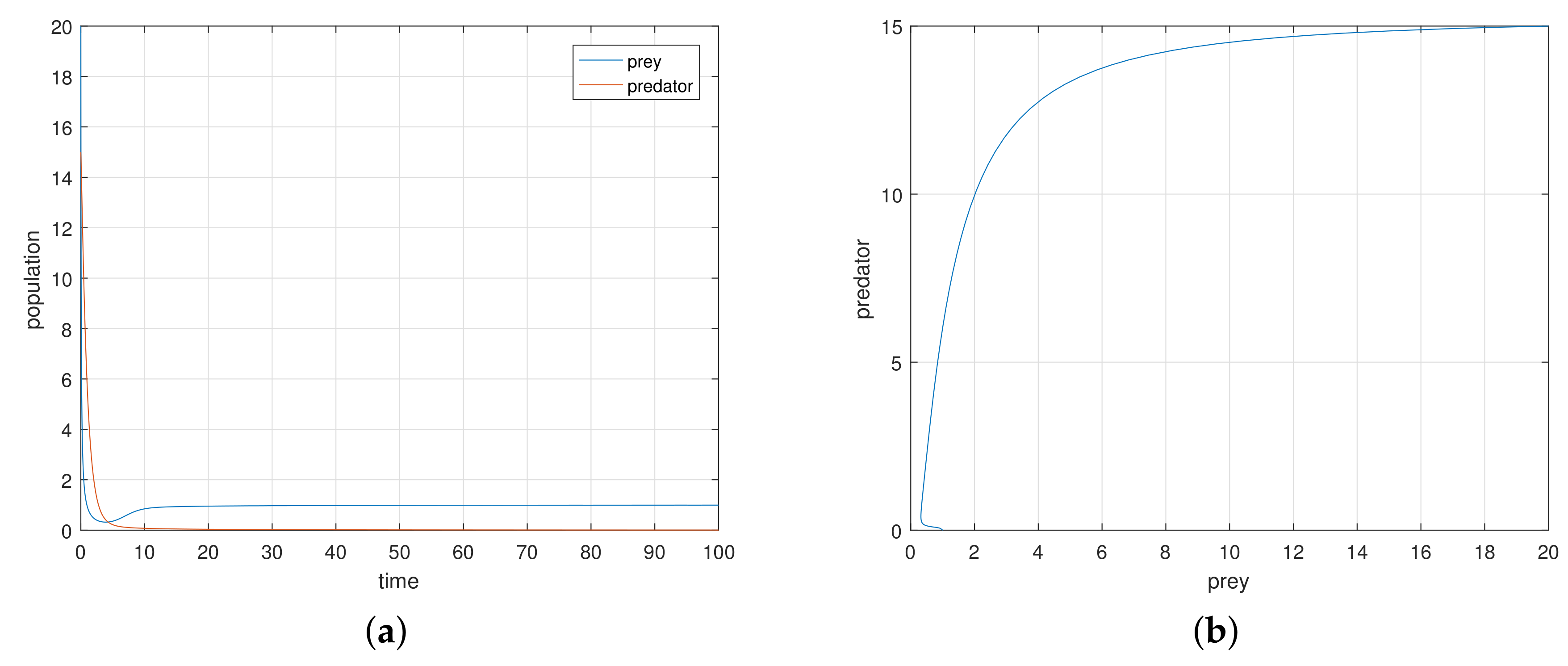
If we increase the consumption ability
of the predator, the system remains stable asymptotically to
. There is a value of
at which the system exhibits a stable periodic oscillation. We take
when the system exhibits a periodic oscillation as illustrated in
Figure 1b. We have taken here several initial states from the basin of attraction
B, and we have obtained the phase-portraits in
Figure 1b. Then the absolute value of the eigenvalue is
. So, at
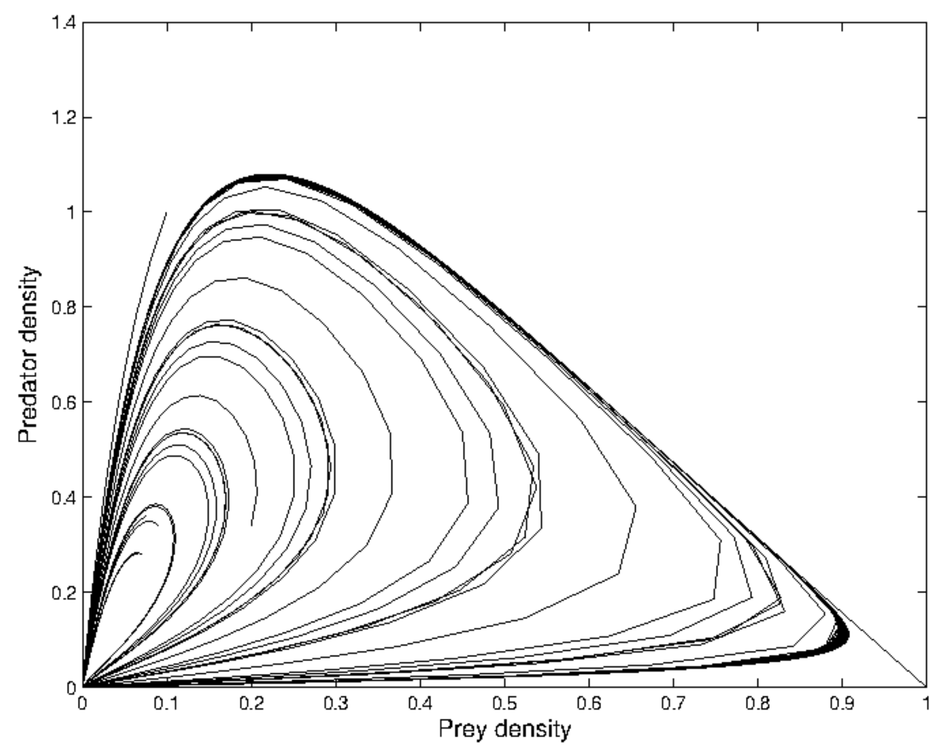
the system has a Hopf type bifurcation where the stable solution becomes periodic. We now tune up the consumption ability of the predator. At
the periodic oscillation losses its stability, and the phase-portrait reduces to an invariant closed curve as illustrated in
Figure 2 around
. Then, the absolute value of the eigenvalue is
.
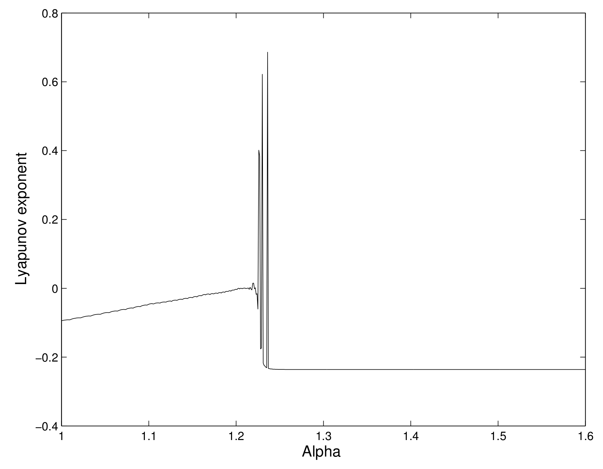
6.1. Order of Chaos by Lyapunov Exponent
We now calculate the maximal Lyapunov exponent of the system, which can give information on chaotic behavior of the system of the 2-dimensional map. A positive Lyapunov exponent indicates that the system exhibits a chaos.
We first give here the mathematical definition of the Lyapunov exponent. We consider the 2-dimensional mapping (
7). A point
is called an
n-cycle point if
The periodic point is stable if the whole orbit
is stable. For an
n-cycle,
The
nth root of this quantity,
is the geometric mean rate of stretching along the entire orbit, and this is defined as characteristic multiplier. If for large
n the logarithm of the above exists, then it is called the Lyapunov exponent based at
. We have calculated the maximal Lyapunov exponent, in which its positive value is the indicator of chaos.
We calculate the maximal Lyapunov exponents for several values of
. We have observed that the Lyapunov exponent is negative for some values of
, and it becomes positive for some other values of
. So, chaos occurs in the system. We have shown the different values of the maximal Lyapunov exponent for different values of the consumption ability
of the predator in
Figure 3.
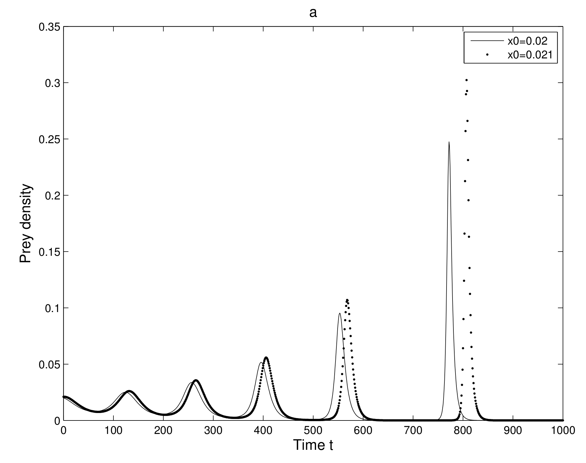
6.2. Existence of Orbit Due to Sensitivity
We analyzed the sensitive dependence of the 2-dimensional map (
7). We considered two neighboring initial conditions
and
and also the initial conditions
and
, where
is very small quantity. This consideration gives us two neighboring orbits in which behavior after some iterations are observed.
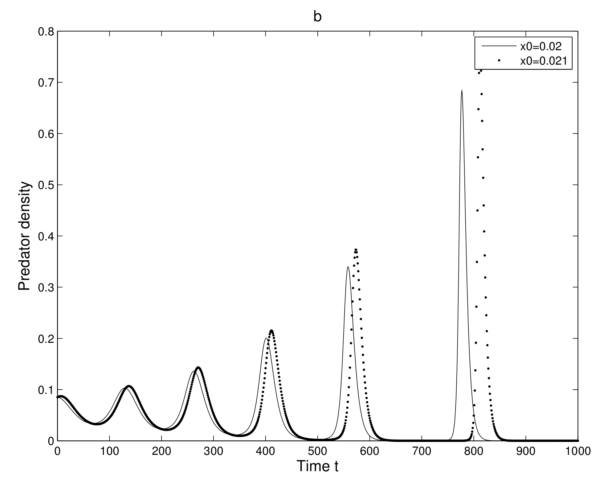
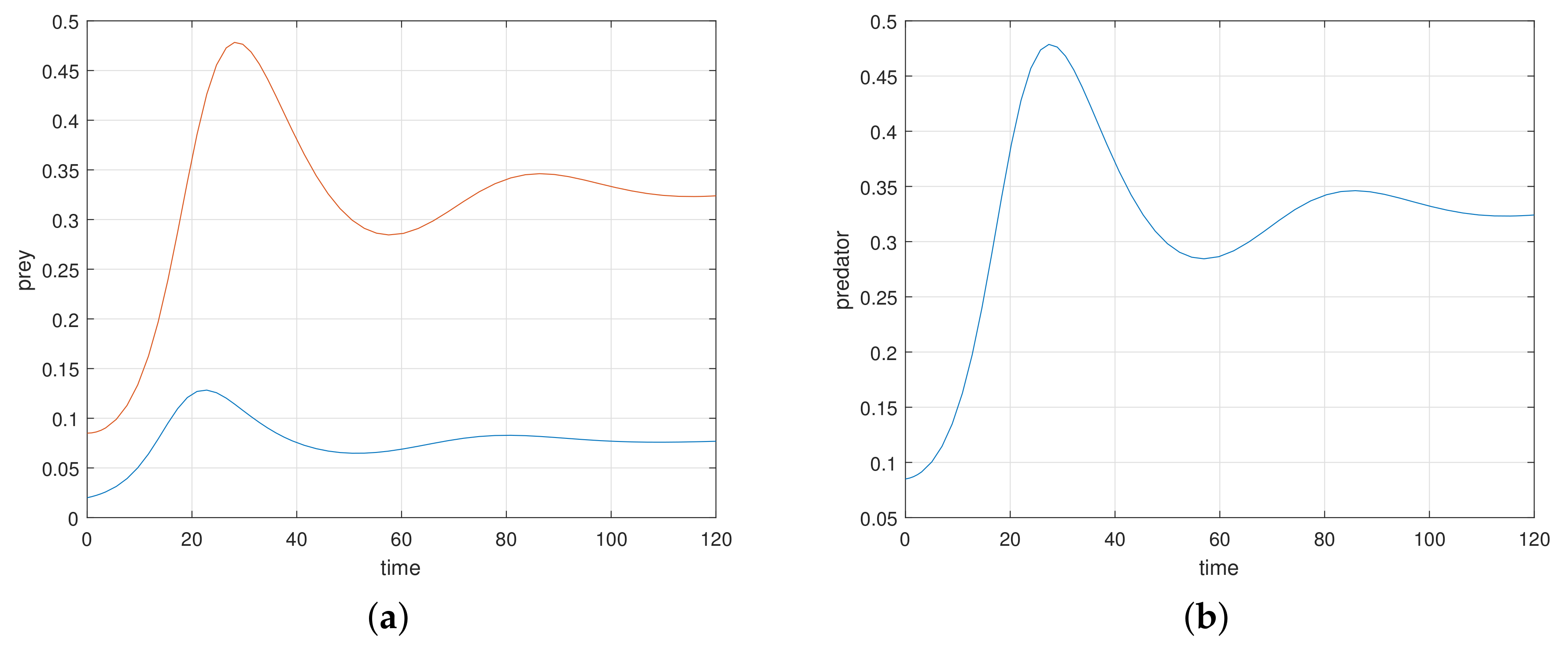
First, we take two neighboring trajectories with initial state
and
. We considered a small change in the
x-coordinate of quantity
only. The time series evolution of the two initial trajectories is shown in
Figure 4a for prey and
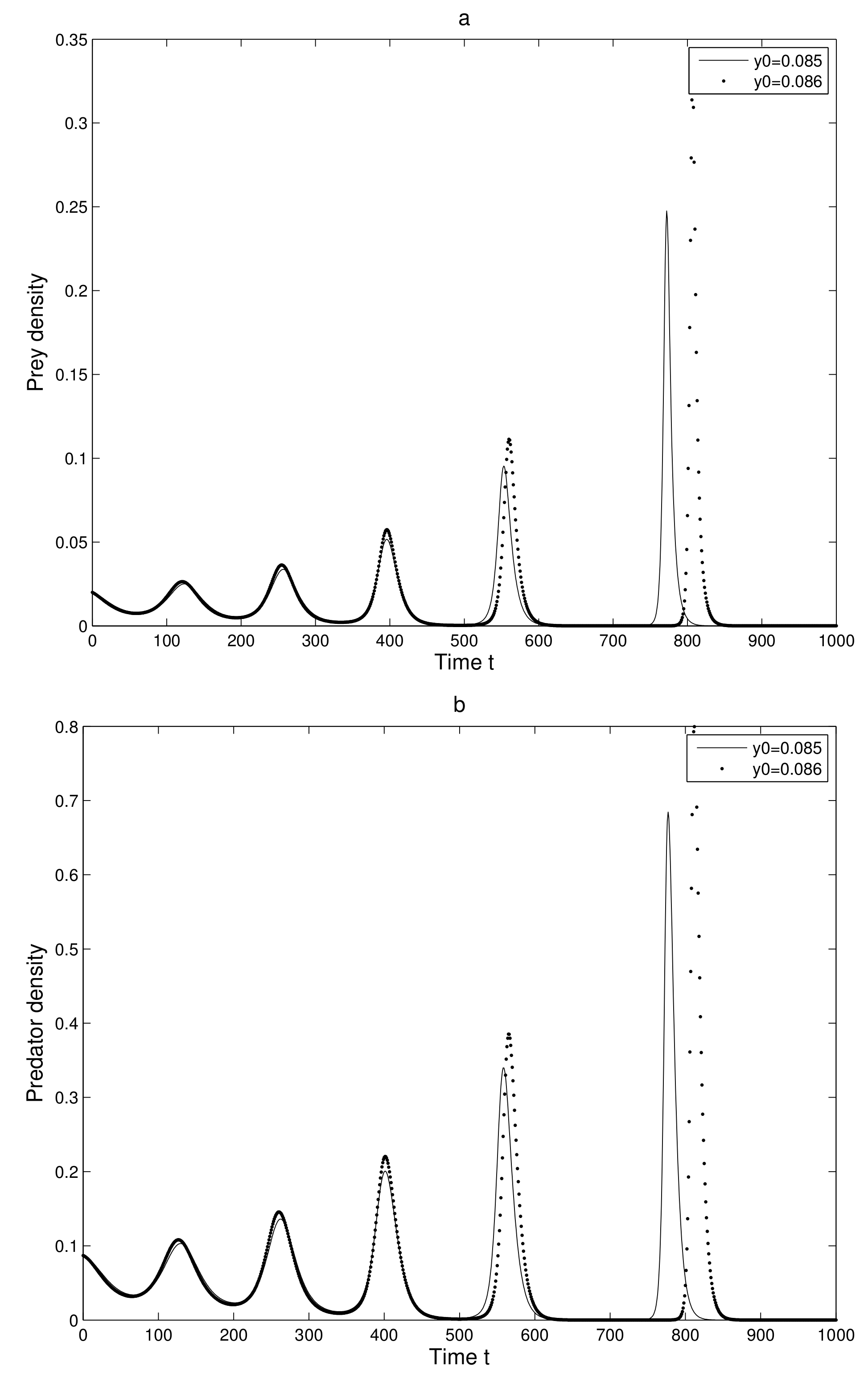
Figure 4b for predator. Initially, the two trajectories overlap, but after some iterations, they show a clear distinction. Secondly, we took two neighboring trajectories with initial state
and
. We considered a small change in the y-coordinate of quantity
only. The time series evolution of the two initial trajectories is shown in
Figure 5a for prey and
Figure 5b for predator. Initially, the two trajectories overlap, but after some iterations, they show a clear distinction.
Thus, we can find a sensitive dependence on initial conditions in the 2-dimensional map. This implies that the long term prediction about the system is not possible. Even in short term prediction of the populations, the small error in the initial conditions can magnify and prediction becomes worthless.
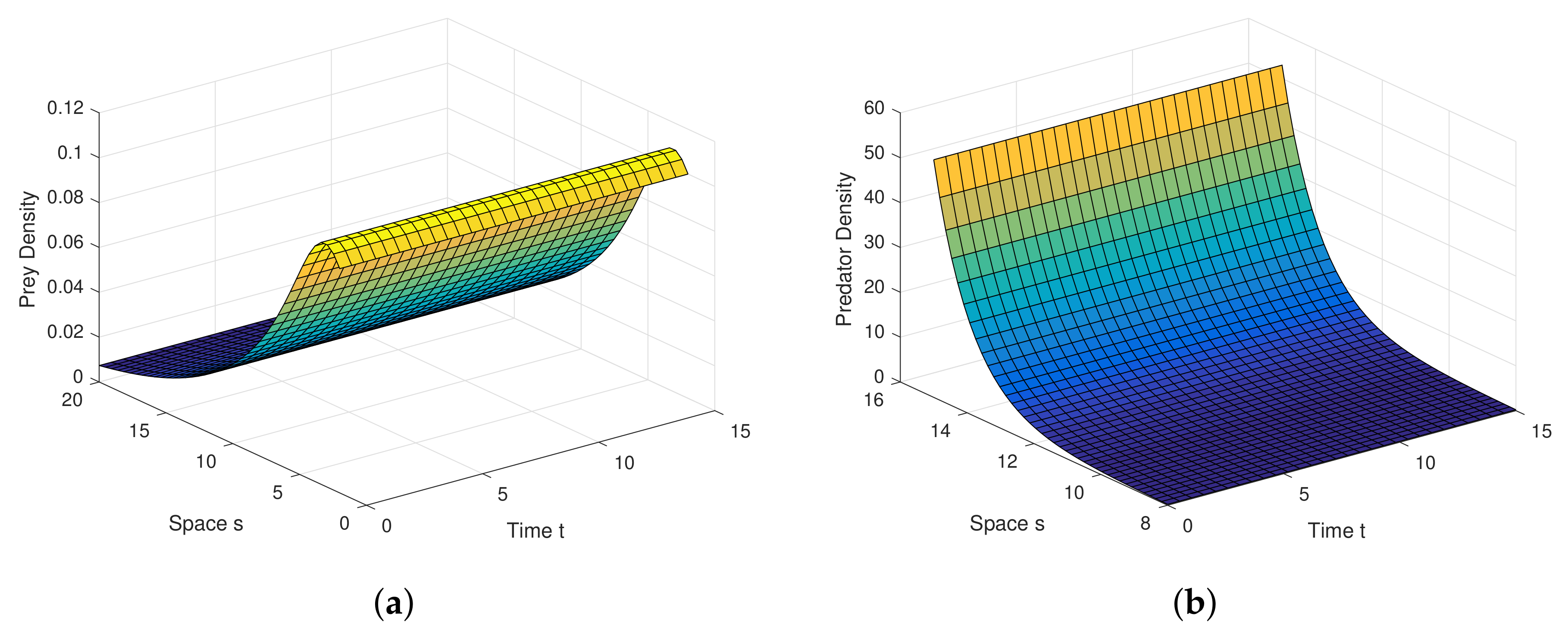
Furthermore, the analytical findings observed in diffusion dynamics and noise process through numerical simulations as follows:
Example 1. For the parameters , , and diffusion coefficients are , . See Figure 6. Example 2. For the parameters , , and diffusion coefficients are , . See Figure 7. Example 3. For the parameters , , and diffusion coefficients are , . See Figure 8. Example 4. For the parameters , , . See Figure 9. Example 5. For the parameters , , . See Figure 10. Example 6. For the parameters , , . See Figure 11. Example 7. For the parameters , , . See Figure 12. Example 8. For the parameters , , , , . See Figure 13. Example 9. For the parameters , , , , . See Figure 14. Example 10. For the parameters , , , , . See Figure 15. 7. Concluding Remarks
To study the discrete type ratio-dependent model, we obtained several results. We considered the Michaelis–Menten type functional response. In finding the fixed point, we saw that the endemic fixed point exists when the consumption ability of the predator precedes some critical value with .
We saw that the origin is stable if the consumption ability of the predator exceeds some critical value when the death rate of the predator precedes 1. When the death rate of the predator exceeds 1, the stability criteria demands the consumption ability to belong in . According to the mathematical analysis, the axial fixed point is stable if the death rate of the predator lies between and . Otherwise, it is a saddle point. The endemic equilibrium state is stable if and unstable if . Here, and are the regions in the positive octant of -space.
The 2-dimensional discrete map exhibits a chaotic behavior as the maximal Lyapunov exponents are positive for some values of . In the continuous time model, such a irregular behavior is not possible.
The dependence of the time series of two species on the initial conditions is evident from the numerical analysis of the model. This type of dependence is not possible in continuous-time model, and the population have no possibility of evolving two different final asymptotic states. For a chaotic trajectory, the nearby trajectories begin to diverge.
The discrete-time model has totally different behavior than the continuous-time model which presents in
Figure 9,
Figure 10,
Figure 11 and
Figure 12. For a low or reasonable death rate in predator system attains stable with attractive oscillations, which is observed in
Figure 12 (with set of parameters
,
,
). For increased death rates in predator, system dynamics and its stability is shown in
Figure 10 and
Figure 11 at various carrying capability and death rates in predator.
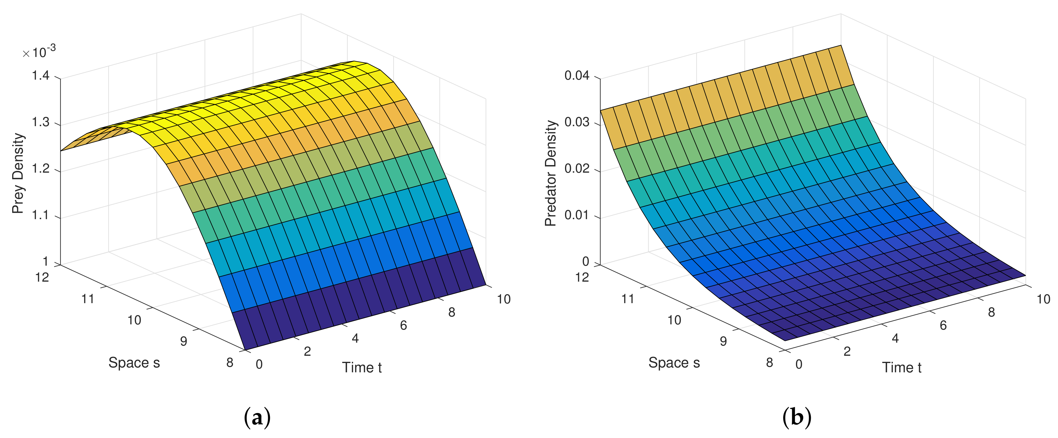
Analytical findings and results in diffusion process are quite interesting in graphical view. Diffusion dynamics are explored highly in simulation.
Figure 6a,b are the graphical outcomes in the process of Diffusion with the coefficients
,
at the interior equilibrium point.
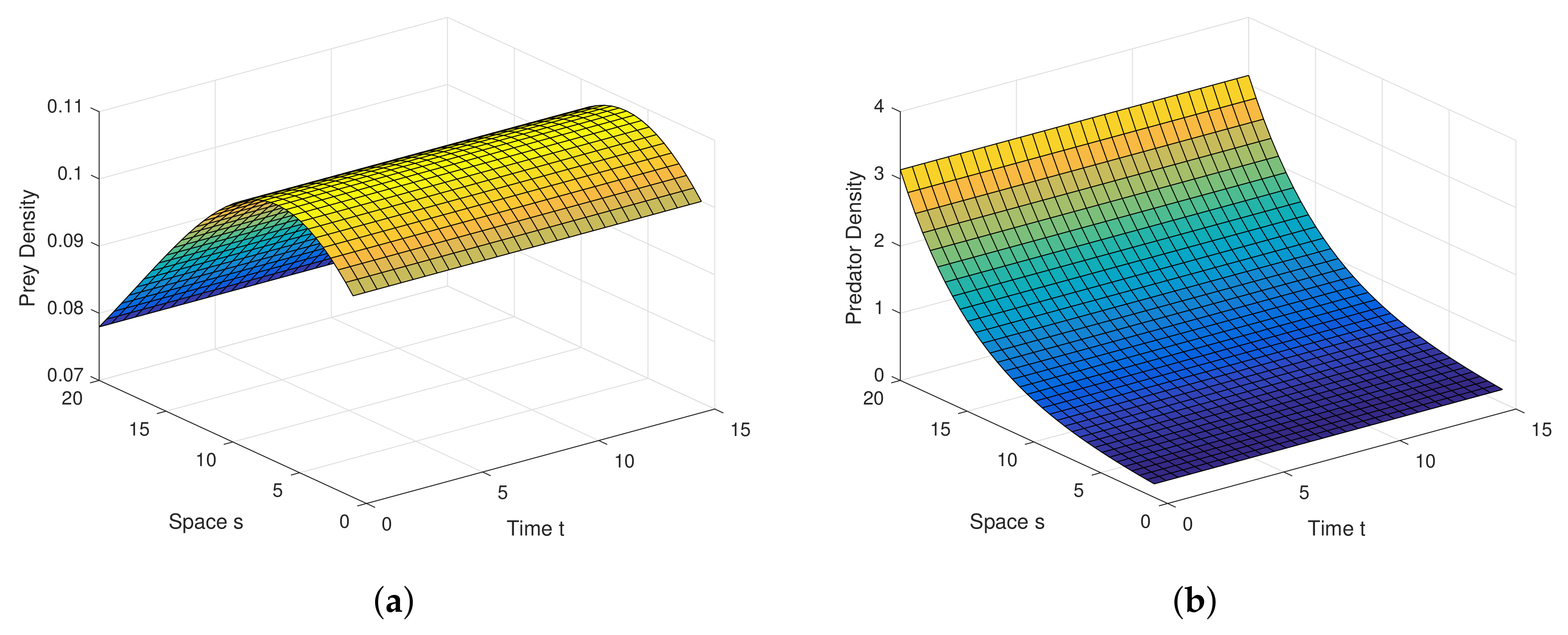
Figure 7a,b are the graphical outcomes in the process of Diffusion with the coefficients
,
at the interior equilibrium point.
Figure 8a,b are the graphical outcomes in the process of Diffusion with the coefficients
,
at the interior equilibrium point. In all these figures, prey exhibits rich dynamics.
Figure 6a,b show clearly, at very low value of diffusion coefficient, the system attains stable rapidly.
Figure 7a,b show clearly, at low value of diffusion coefficient, the system attains stable moderately.
Figure 8a,b show clearly, at high value of diffusion coefficient, the system attains stable little lately. Diffusion process and graphical views are playing a different and attractive role on the proposed model, as well as on any other real world complex scenario.
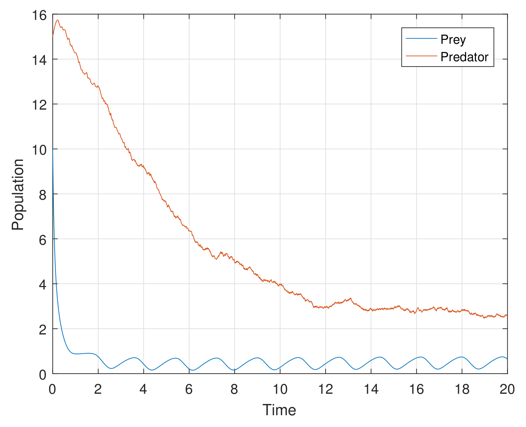
The additional or dynamical forces, like white noise, exhibit interesting results in the process of stochasticity. Stochastic study on any model enhances its stability performance. The perturbation techniques used in the stochastic process help us to strengthen the steadiness of the proposed model. Numerical simulation helps with the rich dynamics of the stochastic study. The analytical findings in the stochastic process are explored attractively through computer simulations in
Figure 13,
Figure 14 and
Figure 15. It is very clear, in graphs at high amplitudes of prey and predator, the system is highly oscillatory, and at low amplitudes of prey and predator (with stochastic parameters
,
), in
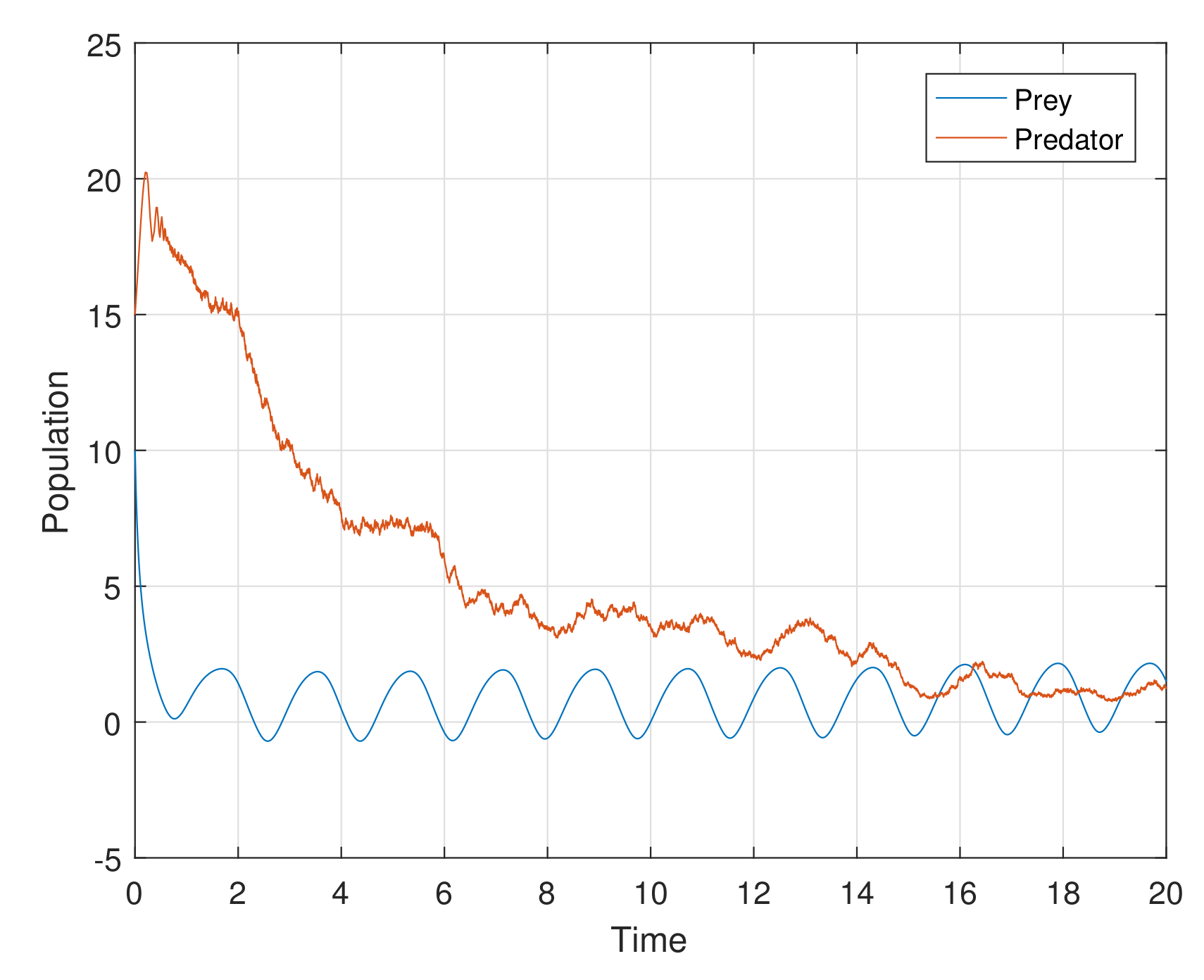
Figure 13, the system attains stablility with low oscillations.
Figure 14 (with stochastic parameters
,
) and
Figure 15 (with stochastic parameters
,
) show that the system attains stablility with high oscillations. Thus, all the analytical findings in different segments are observed, supported, and highly elevated in numerical simulations.


