Improved Differential Evolution Algorithm for Flexible Job Shop Scheduling Problems

Abstract

This research project aims to study and develop the differential evolution (DE) for use in solving the flexible job shop scheduling problem (FJSP). The development of algorithms were evaluated to find the solution and the best answer, and this was subsequently compared to the meta-heuristics from the literature review. For FJSP, by comparing the problem group with the makespan and the mean relative errors (MREs), it was found that for small-sized Kacem problems, value adjusting with “DE/rand/1” and exponential crossover at position 2. Moreover, value adjusting with “DE/best/2” and exponential crossover at position 2 gave an MRE of 3.25. For medium-sized Brandimarte problems, value adjusting with “DE/best/2” and exponential crossover at position 2 gave a mean relative error of 7.11. For large-sized Dauzere-Peres and Paulli problems, value adjusting with “DE/best/2” and exponential crossover at position 2 gave an MRE of 4.20. From the comparison of the DE results with other methods, it was found that the MRE was lower than that found by Girish and Jawahar with the particle swarm optimization (PSO) method (7.75), which the improved DE was 7.11. For large-sized problems, it was found that the MRE was lower than that found by Warisa (1ST-DE) method (5.08), for which the improved DE was 4.20. The results further showed that basic DE and improved DE with jump search are effective methods compared to the other meta-heuristic methods. Hence, they can be used to solve the FJSP.

1. Introduction

Nowadays, the goal of businesses and industry is to reduce costs, and this is affected by production scheduling. Efficient production scheduling can reduce production expenses and time, resulting in on-schedule delivery of goods to customers and a competitive advantage for the firm. The issues of production scheduling concern the sequencing and machine assignment for each order. Owing to the requirement of the modern manufacturing processes for greater flexibility, the job shop scheduling problem (JSP) is an important type of production scheduling; furthermore, the flexible job shop scheduling problem (FJSP) was developed from the classical JSP. Job operations are allocated to every given machine in the production process. It is possible to assign any job to more than one machine as per the machine’s capability and, consequently, constructing an environment that is similar to the actual industry [1]. FJSP is an NP-Hard problem of the combinatorial optimization type, which has a complex solution. Applying a mathematical method to determine the exact algorithms for an optimal solution takes a moderate amount of time and wastes money; in particular, there is a big problem with the great number of variables and the limitations of the method. Metaheuristics are developed to solve FJSP to find a near optimal production schedule and to shorten the time required to solve the problem. It includes Tabu Search, the genetic algorithm (GA), particle swarm optimization (PSO), and ant colony optimization (ACO).

Differential evolution was proposed by Storn and Price [2]. It involves the optimization algorithm by using a population of each generation to search for the solution. Differential evolution calls the member of any generation vector and component of the vector point. Furthermore, it calls a number of points for each vector dimension. Each point can be compared to a gene from the GA method. The method of differential evolution is widely popular owing to its simplicity, various types of solution, and appropriate solutions. In some cases, DE results represent the global optimum.

Hence, in this research, we develop the differential evolution algorithm for solving in the flexible job shop scheduling problem with the target of minimizing the makespan.

This paper is structured as follows: In Section 2, the literature review is presented; Section 3 presents the mathematical model of the FJSP; Section 4 describes the general structure of the DE; Section 5 presents the results of the experiment on DE to solve the FJSP; Section 6 presents the comparison of DE with other metaheuristics; and Section 7 presents the conclusions and suggestions.

2. Literature Review

2.1. Flexible Job Shop Scheduling Problems by Using Other Metaheuristic Methods

To summarize the relevant literature and research on the solution to the flexible job shop scheduling problem by using metaheuristics, Xia and Wu [3] studied a hybrid of the PSO and SA methods for multiple purposes. Kanate [4] researched the development of a metaheuristic called the makespan tree for sequencing jobs on machines. Subsequently, two metaheuristics, the genetic algorithm and particle swarm optimization, were developed. Both metaheuristics use the makespan tree as a part of their method to solve the flexible job shop problems with the objective of minimizing the makespan. The findings for the job scheduling problems showed that the makespan tree outperformed the non-delay by 11.80%, improved the earliest finish time by 13.60%, and reduced the shortest processing time by 17.41%. In comparison, PSO had better results than GA by 0.97%. Tang et al. [5] researched the use of a hybrid algorithm for the flexible job-shop scheduling problem by combining chaos particle swarm optimization with the genetic algorithm in order to minimize the makespan. Wannaporn and Arit [6] applied the modified genetic algorithm to the flexible job-shop scheduling problem. This included the following processes: (1) Selecting chromosomes by the fuzzy roulette wheel selection method; (2) operating the crossover by the cluster-crossover operator to calculate the similarity between chromosomes for the crossover; (3) processing mutations using the mutation-local search operator to determine the diversity of the population, resulting in an optimal solution. The objective of this research was to minimize the makespan. Thanyaporn et al. [7] developed and improved the mixed integer programming (MIP) for an advanced planning and scheduling (APS) problem as a technique for production planning and scheduling. Its various considered constraints were the machine capacity, operation sequence, multi-machine due dates, multi-order, and product structure, comprising multiple steps and items. Each item could be processed by any given set of machines, and there was an extension to involve the considered constraints as a preventive maintenance time window. The objective was to minimize the total costs from idle production time, earliness, and tardiness, and furthermore, to optimize production scheduling. Examples of solutions were presented in four models which were (1) APS1, APS without alternative machines, (2) APS1PM, APS without alternative machines and PM, being similar to model 1 but with preventive maintenance included, (3) APS2, APS with alternative machines, and (4) APS2PM, APS with alternative machines and PM, being similar to model 3 but with preventive maintenance included. Hamid et al. [8] studied the machine scheduling in production—a content analysis. Which found that there were 132 surveyed papers regarding machine scheduling problems in production. The results were applied as an approach for proposing future research. It was found that, generally, the objective was to minimize the makespan. For the problem-solving approach, simple heuristics, as the shortest processing time first (SPT), and meta-heuristics, as the genetic algorithm, were employed. Li and Gao [9] studied an effective hybrid genetic algorithm and Tabu Search for flexible job shop scheduling problem. Luan et al. [10] studied improved whale algorithm for solving the flexible job shop scheduling problem and Li et al. [11] studied the hybrid artificial bee colony algorithm with a rescheduling strategy for solving the flexible job shop scheduling problems.

2.2. Flexible Job Shop Scheduling Problems by Using Differential Evolution Algorithm

Based on a study of the literature and research regarding the solutions to flexible job shop scheduling problems by using the differential evolution algorithm, Wisittipanich [12] proposed the application of adapted differential evolution algorithms to minimize the makespan in the FJSP. The modification of algorithms aimed to improve the efficiency of original DE by balancing its exploration and exploitation abilities to avoid the common problem of premature convergence. The first adapted DE was called the DE with subgroup strategy. In this algorithm, the population is divided into groups, and the population in each group employs different strategies to search for the new solution simultaneously in order to extract the strength of any strategy and compensate for the weakness of each strategy. This led to an increase in the overall performance efficiency. The second adapted DE was the DE with the switching strategy. This algorithm allowed the entire population to change searching strategies when there was no improvement to the solution. Thus, the chance of being trapped at a local optimum was decreased. The efficiency of two modified DEs was examined in solving an experimental problem and compared with the result of the original DE. The solutions provided by both modified DE algorithms were comparable or of a higher quality than the solutions from the original DE. Yuan and Xu [13] studied flexible job shop scheduling using hybrid differential evolution algorithms. Hybridization comprised the development of a mechanism to use the discrete differential evolution algorithm to solve the flexible job shop scheduling problem and second, enhancement of the local search ability in the DE framework. The objective was to find minimize the makespan. Bhaskara et al. [14] on the use of the differential evolution algorithm for the flexible job shop scheduling problem, applied the local search algorithm with the objective of minimizing the makespan.

2.3. Differential Evolution Algorithm for Solving Other Problems

The differential evolution algorithm is perceived as a modern method. It has become a favorable method to employ in various areas including operational research problems, such as application in the blocking flow shop scheduling problems to reduce production time [15]. Furthermore, in was applied in job shop production. Zhang et al. [16] adapted this method to deal with the job shop problem in order to minimize the total tardiness. For applications in the supply chain management problem, in particular, for the vehicle routing problem in the supply chain, the relevant studies have been carried out with different objectives and constraints under various conditions. For example, Cao and Lai [17] adapted the method to the open vehicle routing problem with fuzzy demands to reduce the total traveled distance. Lai and Cao [18] applied the method to solve the VRP with pickups and deliveries and time windows aimed at minimizing the total traveled distance. Xu and Wen [19] employed the DE in the unidirectional logistics distribution vehicle routing problem with no time windows and achieved the shortest total distance. By adapting DE with the agricultural management problem, Cruz et al. [20] applied the optimal control problem to determine the optimal control of nitrogen gas in lettuce. Moreover, DE was employed in a proposal on crop planning using the multi-objective differential evolution algorithm. This study had the objective of minimizing irrigation water usage and maximizing the total yield and net profit planting under various conditions [21]. DE was further applied to other problems, for example, in the electric power system, it was used to solve the optimal power flow, resulting in voltage stability enhancement and cost minimization [22]. In the wireless sensor network system, DE was proposed to prolong the lifetime of the system by preventing it from overloading [23]. An adaptation of DE, moreover, was used in the chemical industry in order to determine the optimal criteria for a chemical process [24].

3. Flexible Job Shop Scheduling Problem Pattern and Mathematical Model

We only focused on the FJSP in this study, and the details of the problem are as follows:

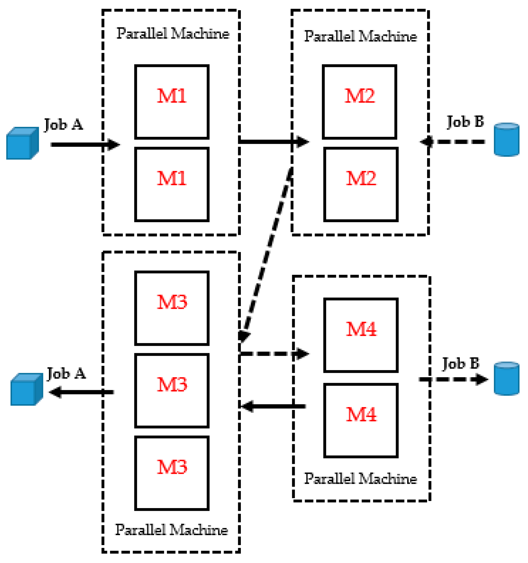
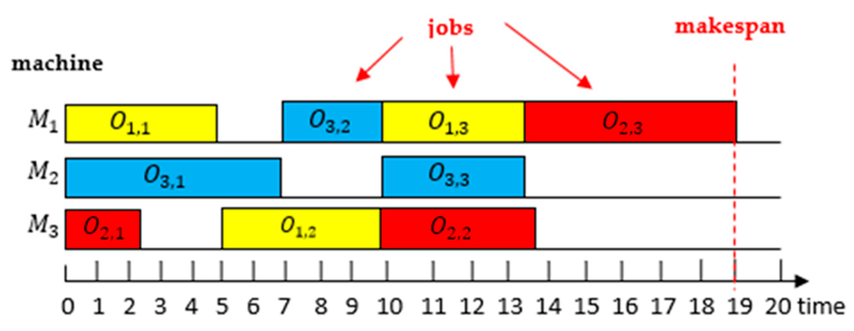
3.1. Flexible Job Shop Scheduling Problem (FJSP)

This production system is similar to the job shop scheduling problem but with more flexibility. As an explanation, any job includes a specific operation that can be processed by 1 or more machines owing to the various capabilities of the individual machine. As shown in

Table 1. Example of flexible job shop scheduling problem pattern.

Job	Operation	Machines
		M1	M2	M3
J1	O1,1	5	-	3
	O1,2	-	5	10
	O1,3	5	9	-
J2	O2,1	-	10	7
	O2,2	20	6	-
	O3,3	2	-	11
J3	O3,1	2	5	4
	O3,3	2	5	10

, there are 3 jobs, each with a different set of operations. Every operation is allowed to select any machine from a given set, for example, in job 2, operation 1 can be performed on 2 machines, with M2 processing 10 time units and M3 processing 7 time units, while M1 shows “-”, referring to an inability to operate.

Figure 1 shows the general pattern of flexible job shop scheduling problem systems, which consist of a system with C work stations. In each work station, there will be a number of identical parallel machines. Each work station has its own specific route and can choose to perform the tasks assigned to one of the parallel machines and can be at the same work station. Considering the complexity of the model, the model of the flexible job shop scheduling problem systems that allows for recursive operation is the most redundant model.

To measure the production scheduling efficiency, there are various effective evaluations based on the production characteristics such as determining the minimization of the makespan (C_max), the number of tardy jobs, and the maximum lateness. This paper employed the minimized makespan (C_max) for evaluation in accordance with Equation (1). While C1, C2, …, C_p are possible solutions to produce scheduling, the solution resulting in the longest processing time was selected. Moreover, Z refers to the objective of production scheduling—to achieve the lowest value—as described in Equation (1). Figure 2 shows a sample of solutions from the total processing time of entire jobs:

Minimize Z = f (C₁, C₂, …, C_p).

(1)

The relative error is the difference between the measured and actual values, and it is generally expressed as a percentage (%). When the measured value is proximate to the actual value, this indicates high correctness or accuracy. The relative error is calculated using Equation (2), as follows;

$$\%\mathrm{Relative}\mathrm{Error}:\mathrm{RE}=\frac{{\mathrm{C}}_{\min }-\mathrm{BKS}}{\mathrm{BKS}}\times 100$$

(2)

where C_min is the optimal solution to the algorithm, and BKS is the best known solution.

3.2. Mathematical Model of the Flexible Job Shop Scheduling Problem

The mathematical model of the FJSP, proposed by Kanate [4], includes many relevant binary variables, which are as follows:

3.2.1. Indices

$i$    Machine

$j,k$  Job

$h, l$  Operation

3.2.2. Parameter

$M$    Mathematically large real number

$P_{i,j,h}$ Processing time for operation $h$ of job $j$ on machine $i$

$O_{i,j,h}$ Operation $h$ of job $j$ on machine $i$

$a_{i,j,h}$ Constant to define if job $j$ at operation $h$ is able to be processed by $i$—equal to 1 for the ability to process and 0 for the inability to process

3.2.3. Decision Variables

$C_{max}$  Makespan

$t_{j,h}$   Start time of the processing operation $h$ of job $j$ on any machine

$f_{j,h}$   Finish time of the processing operation $h$ of job $j$ on any machine

$y_{i,j,h}$   Binary variable equal to 1 while processing operation $h$ of job $j$ on machine $i$

$X_{i,j,h,k,l}$ Binary decision variable equal to 1 while processing operation $h$ of job $j$ on machine $\left(O_{i,j,h}\right)$, which comes before operation $l$ of job $k$ on machine $i$ $\left(O_{i,k,l}\right)$.

The mathematical model of the flexible job shop scheduling problem can be written as:

$$\begin{array}{c}\mathrm{Minimize}{C}_{max}=\max \left\{C_i\right\},i=1,2,3,\dots ,n\\ \mathrm{st}.\end{array}$$

(3)

$$t_{j,h}+y_{i,j,h}\times P_{i,j,h}\le f_{i,h}; \forall \left(i,j,h\right)$$

(4)

$$f_{j,h}\le t_{j,h+1}; \forall \left(j,h\right)$$

(5)

$$f_{j,h}\le C_{max}; \forall \left(j,h\right)$$

(6)

$$y_{i,j,h}\le a_{i,j,h}; \forall \left(i,j,h\right)$$

(7)

$$t_{j,h}+P_{i,j,h}\le t_{k.l}+\left(1-x_{i,j,h,k,l}\right)M; \forall \left(i,j,h,k,l\right)$$

(8)

$${\displaystyle \sum }_i{y}_{i,j,h}=1; \forall \left(h,j\right)$$

(9)

$${\displaystyle \sum }_j{\displaystyle \sum }_h{x}_{i,j,h,k,l}=y_{i,k,l}; \forall \left(i,k,l\right)$$

(10)

$${\displaystyle \sum }_k{\displaystyle \sum }_j{x}_{i,j,h,l,k}=y_{i,j,h}; \forall \left(i,j,h\right)$$

(11)

$$x_{i,j,h,j,h}=0; \forall \left(i,j,h\right)$$

(12)

$$t_{j,h}\ge 0; \forall \left(j,h\right)$$

(13)

$$f_{j,h}\ge 0; \forall \left(j,h\right)$$

(14)

$$y_{i,j,h}\in \left\{0,1\right\}$$

(15)

$$x_{i,j,h,k,l}\in \left\{0,1\right\}$$

(16)

Equation (3) is a target equation to produce the minimum makespan, in order to reduce the production time, contributing to lower costs and product delivery time. Next, Equations (4) and (5) restrict the order based on the priority order in which each job is processed (precedence constraint). Equation (6) imposes a constraint on the makespan, whereby all job operations must be finished in a time less than or equal to the makespan. For Equation (7), only machines available for processing can be selected. Equation (8) is used to ensure that each machine can process, at most, one job at a time. Constrained by Equation (9), any job operation can be assigned to process on one machine only. Equations (10) and (11) create the sequence of job priority on machine $i$—Equation (10) selects the predecessor job and Equation (11) selects the next job. Equation (12) is the constraint that ensures that each job operation cannot be processed before its release time on machine $i$. Subsequently, Equations (13) and (14) restrict the start and finish times of every job to positive real numbers. Furthermore, Equations (15) and (16) specify $y_{i,j,h}$ and $x_{i,j,h,k,l}$ as binary variables.

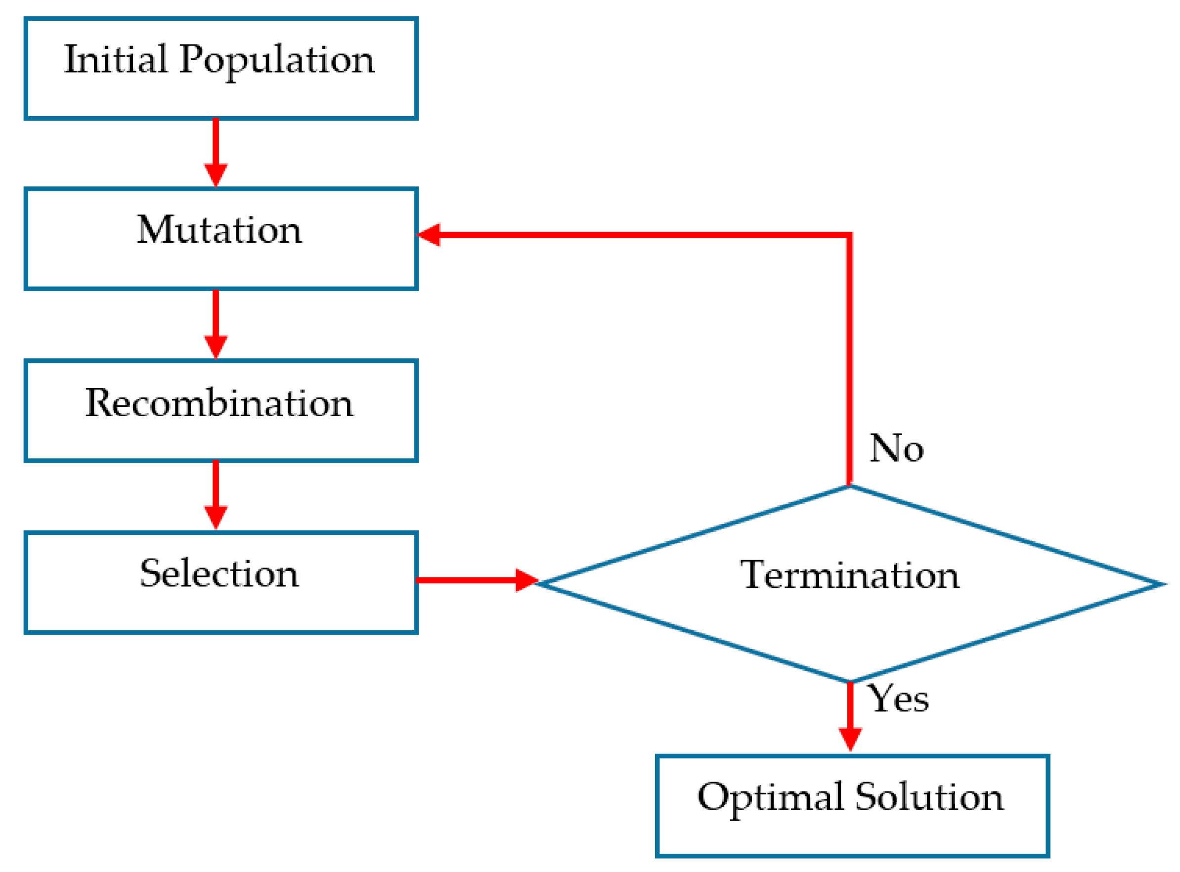
4. General Differential Evolution Algorithm

The general differential evolution algorithm has general procedures [25], as shown in Figure 3.

The procedures of the differential evolution algorithm consist of (1) the initial population, and (2) mutation to generate mutant vector by differentiating a dimension of the vector. The calculation for mutating a vector’s dimensions is shown in Equation (17):

$$V_{m,n,G}=X_{r1,n,G}+F\left(X_{r2,n,G}-X_{r3,n,G}\right)$$

(17)

where m is the number of vectors of each generation, n is vector dimension, G is the iteration round, such as round 1, 2, or 3, and r1, r2, and r3 are 3 random vectors. F is the scaling factor, where $V_{m,n,G}$ is a mutant vector for vector m at vector dimension n in iteration round G. Moreover, $X_{r1,n,G}$ is firstly the random target vector at dimension n in iteration round G. $X_{r2,n,G}$ and $X_{r3,n,G}$ are, respectively, the second and third random target vectors. Thus, the mutant vector of vector m at dimension n in round G equals the value of target vector r1 at dimension n round G plus scaling factor F times the difference between target vectors r2 and r3. (3) Recombination of the trial vector is generated by exchanging vector dimensions. The equation employed for generating a trial vector is Equation (18):

$$U_{m,n,G}=\{\begin{array}{c}{V}_{m,n,G} if ran{d}_{mn}\le CR or D_m=D_{m_{rand}}\\ X_{m,n,G}, else.\end{array}$$

(18)

where $U_{m,n,G}$ is the trial vector of vector m at dimension n in round G, $ran{d}_{mn}$ is a random real number between [0, 1] of vector m at dimension n, CR refers to the crossover rate, D_m is the dimension of vector m. Furthermore, $D_{m_{rand}}$ denotes a random integer number of vector m in the range [1, N], where N is the vector size. Consequently, the value of trial vector m in dimension n in iteration round G equals the mutant vector when there is a random number of vector m at dimension n that is less than CR; in other words, $D_{m_{rand}}$ equals D_m. (4) The formula for selecting a target vector for the next round described in Equation (19). To solve the equation for the minimum target value (minimization), the less than or equal to sign is used:

$$X_{m,n,G+1}=\{\begin{array}{c}{U}_{m,n,G} if f\left(U_{m,n,G}\right)\le f\left(X_{m,n,G}\right)\\ X_{m,n,G}, else.\end{array}$$

(19)

where, $X_{m,n,G+1}$ is the target vector m at dimension n in round G + 1, where the vector with a better fitness function value is selected in comparison with the value of the target vector and trial vector in round G.

4.1. Procedure of FJSP by Using Differential Evolution Algorithm

The procedure of FJSP uses the general differential evolution algorithm. The values used in the calculation must be set. The variables are as follows: Iterate = round, NP = number in population, F = scaling factor, and CR = crossover rate. In this problem’s calculation, these suitable variables were set from the experiment as Iterate = 1, NP = 5, F = 0.8, and CR = 0.8. The general differential evolution algorithm “DE/rand/1” and binomial crossover were used in the calculation.

4.1.1. Calculation Using the General Differential Evolution Algorithm DE/rand/1 and Binomial Crossover

The flexible job shop scheduling problem in

Table 2. Sample problems of Kacem et al. [26,27].

45. 35. 1 2 2 5 3 4 4 1 5 2 5 1 5 2 4 3 5 4 7 5 5 5 1 4 2 5 3 5 4 4 5 5 35. 1 2 2 5 3 4 4 7 5 8 5 1 5 2 6 3 9 4 8 5 5 5 1 4 2 5 3 4 4 54 5 5 45. 1 9 2 8 3 6 4 7 5 9 5 1 6 2 1 3 2 4 5 5 4 5 1 2 2 5 3 4 4 2 5 4 5 1 4 2 5 3 2 4 1 5 5 25. 1 1 2 5 3 2 4 4 5 12 5 1 5 2 1 3 2 4 1 5 2

provides the details of the processing time on each machine. By explanation,

Row 1 indicates the numbers of jobs and machines, including 4 jobs and 5 machines.

Row 2 shows the data on job 1, comprising 3 operations. In operation 1, there are 5 available machines, which are machine 1 with a processing time of 2, machine 2 with a processing time of 5, machine 3 with a processing time of 4, machine 4 with a processing time of 1, and machine 5 with a processing time of 2. Operation 2 includes machine 1 with a processing time of 5, machine 2 with a processing time of 4, machine 3 with a processing time of 5, machine 4 with a processing time of 7, and machine 5 with a processing time of 5. Furthermore, operation 3 has machine 1 with a processing time of 4, machine 2 with a processing time of 5, machine 3 with a processing time of 5, machine 4 with a processing time of 4, and machine 5 with a processing time of 5.

Rows 3–5 show the data on jobs 2–4. The processing time of each operation can be likewise described, as shown in row 2, and put into categories, as shown in

Table 3. Sample problem with four jobs and five machines.

Jobs	Operations	Machines
		M1	M2	M3	M4	M5
J1	O1,1	2	5	4	1	2
	O1,2	5	4	5	7	5
	O1,3	4	5	5	4	5
J2	O2,1	2	5	4	7	8
	O2,2	5	6	9	8	5
	O2,3	4	5	4	54	5
J3	O3,1	9	8	6	7	9
	O3,2	6	1	2	5	4
	O3,3	2	5	4	2	4
	O3,4	4	5	2	1	5
J4	O4,1	1	5	2	4	12
	O4,2	5	1	2	1	2

.

To improve the solution to round 1, the following procedure is completed:

Step 1: Generate the initial population

The initial population is randomized from a number between [0, 1], where the dimension or position (D) equals the number of operations (12), and the number of populations (P; 5) results in the target vector of a sample, as shown in

Table 4. Target vectors of sample problems.

NP	Dimensions, D
	1	2	3	4	5	6	7	8	9	10	11	12
1	0.55	0.32	0.70	0.12	0.64	0.89	0.96	0.81	0.38	0.55	0.27	0.71
2	0.17	0.80	0.94	0.93	0.44	0.36	0.77	0.35	0.13	0.42	0.17	0.11
3	0.42	0.35	0.15	0.61	0.10	0.34	0.93	0.51	0.08	0.59	0.63	0.50
4	0.65	0.72	0.30	0.58	0.02	0.74	0.59	0.17	0.14	0.07	0.73	0.31
5	0.72	0.32	0.04	0.20	0.89	0.28	0.42	0.67	0.15	0.49	0.09	0.81

.

Step 2: Differentiation of a dimension or mutation

Three vectors, $r_1$, $r_2$, $\mathrm{and} r_3$, are randomly picked from the total population equal to 5 in order to generate a mutant vector of the entire 5 target vectors. As indicated by the sample problems, the randomized vectors ($r_1$, $r_2$, $r_3$) from target vector 1 consist of vectors 2, 5, and 3. The other concerned target vectors are demonstrated in

Table 5. Randomized vectors $r_1$, $r_2$, $\mathrm{and} r_3$.

Random Vector	r1	r2	r3
1	2	5	3
2	3	3	5
3	4	2	2
4	5	1	1
5	1	4	4

.

Calculation of the mutant vector ($V_{m,n,G}$) can be performed by substituting the randomized vector into Equation (20). Thus, the mutant vectors of sample problems are presented in

Table 6. Mutant vectors of sample problems in round 1.

Mutation	1	2	3	4	5	6	7	8	9	10	11	12
1	0.77	0.74	0.42	0.11	2.02	0.24	−0.25	0.67	0.27	0.22	−0.91	0.73
2	0.80	0.13	0.74	0.24	1.78	0.50	−0.47	0.04	1.81	0.38	−0.43	0.37
3	0.16	0.70	0.56	0.61	1.45	0.43	−0.74	0.24	1.30	−0.08	0.02	0.40
4	0.81	0.43	0.24	−0.36	0.03	0.09	0.97	0.69	−0.70	1.04	1.19	1.04
5	0.87	1.30	0.65	0.69	1.05	1.39	0.23	−0.86	1.31	0.60	0.31	0.91

.

$$V_{m,n,G}=X_{r1,n,G}+F\left(X_{r2,n,G}-X_{r3,n,G}\right)$$

(20)

Step 3: Crossover

The number in the range [0, 1] at the target vector position is randomly picked and is comparative to the crossover rate (CR) predefined for the crossover.

Table 7. Random numbers for the crossover.

Vector	1	2	3	4	5	6	7	8	9	10	11	12
1	0.83	0.05	0.75	0.80	0.95	0.39	0.29	0.60	0.30	0.44	0.59	0.65
2	0.68	0.36	0.48	0.47	0.70	0.96	0.04	0.76	0.64	0.42	0.16	0.44
3	0.32	0.40	0.97	0.38	0.63	0.69	0.71	0.92	0.65	0.83	0.92	0.49
4	0.56	0.18	0.06	0.38	0.47	0.23	0.11	0.85	0.80	0.30	0.65	0.02
5	0.81	0.35	0.70	0.50	0.89	0.89	0.84	0.29	0.01	0.21	0.41	0.83

shows the random numbers for the crossover.

Subsequently, the trial vector is calculated with Equation (21). In comparison, if a random number is less than or equal to CR = 0.8, the mutant vector in the same position will be selected as the obtained trial vector of that position. For differential cases, the target vector in the same position is the answer to the trial vector of the concerned position.

Table 8. Trial vectors from round 1.

Trial Vector	1	2	3	4	5	6	7	8	9	10	11	12
1	0.55	0.74	0.42	0.12	0.64	0.24	−0.25	0.67	0.27	0.22	−0.91	0.73
2	0.80	0.13	0.74	0.24	1.78	0.50	−0.47	0.04	1.81	0.38	−0.43	0.37
3	0.16	0.70	0.56	0.61	1.45	0.43	−0.74	0.24	1.30	−0.08	0.02	0.40
4	0.65	0.72	0.30	0.58	0.02	0.74	0.59	0.17	0.14	0.07	0.73	0.31
5	0.72	0.32	0.04	0.20	0.89	0.28	0.42	0.67	0.15	0.49	0.09	0.81

shows the obtained trial vectors.

$${\mathrm{U}}_{\mathrm{ji},\mathrm{G}+1}=\{\begin{array}{c}{\mathrm{V}}_{\mathrm{ji},\mathrm{G}+1} if\left(randb\left(j\right) \le CR\right) or j = rnbr \left(i\right) \\ {\mathrm{X}}_{\mathrm{ji},\mathrm{G}} if\left(randb\left(j\right) > CR\right) or j \ne rnbr \left(i\right) \end{array}$$

(21)

Step 4: Fitness Evaluation

To decode the value of each dimension, the values are sorted based on the rank order value (ROV) in ascending order. Furthermore, the values are positioned in accordance with the vector order, as described in

Table 9. Results of decoding.

Vector	11	7	4	10	6	9	3	1	5	8	12	2
1	−0.91	−0.25	0.12	0.22	0.24	0.27	0.42	0.55	0.64	0.67	0.73	0.74
Oi,j	1, 1	1, 2	1, 3	2, 1	2, 2	2, 3	3, 1	3, 2	3, 3	3, 4	4, 1	4, 2

.

As a consequence of the sequencing machine operation, the machine with the earliest completion time is selected. If the machine operation consumes time equally, selection becomes random. This is described in

Table 10. Results of the sequencing machine operation.

Vector	1	2	3	4	5	6	7	8	9	10	11	12
1	0.55	0.74	0.42	0.12	0.64	0.24	−0.25	0.67	0.27	0.22	−0.91	0.73
Oi,j	3,2	4,2	3,1	1,3	3,3	2,2	1,2	3,4	2,3	2,1	1,1	4,1
M	2	2	4	1	1	5	2	4	3	1	4	1
PT	1	1	6	4	2	5	4	1	4	2	1	1

and illustrated by the Gantt chart in Figure 4.

Figure 4 presents a Gantt chart for solving the problem of a sample with 4 jobs, 5 machines, 12 operations, and a makespan of 17. The machines on the critical part are machines 1, 5, and 2 which consequentially interfere with solutions using the local search method.

Step 5: Selection

By comparing the fitness factor values of target vectors (

Table 11. Target vectors of round 1.

Target Vector	1	2	3	4	5	6	7	8	9	10	11	12	Target
1	0.55	0.32	0.70	0.12	0.64	0.89	0.96	0.81	0.38	0.55	0.27	0.71	21
2	0.17	0.80	0.94	0.93	0.44	0.36	0.77	0.35	0.13	0.42	0.17	0.11	20
3	0.42	0.35	0.15	0.61	0.10	0.34	0.93	0.51	0.08	0.59	0.63	0.50	22
4	0.65	0.72	0.30	0.58	0.02	0.74	0.59	0.17	0.14	0.07	0.73	0.31	24
5	0.72	0.32	0.04	0.20	0.89	0.28	0.42	0.67	0.15	0.49	0.09	0.81	19

) with the fitness factor values of the trial vectors (

Table 12. Trial vectors of round 1.

Trial Vector	1	2	3	4	5	6	7	8	9	10	11	12	Target
1	0.55	0.74	0.42	0.12	0.64	0.24	−0.25	0.67	0.27	0.22	−0.91	0.73	18
2	0.80	0.13	0.74	0.24	1.78	0.50	−0.47	0.04	1.81	0.38	−0.43	0.37	25
3	0.16	0.70	0.56	0.61	1.45	0.43	−0.74	0.24	1.30	−0.08	0.02	0.40	16
4	0.65	0.72	0.30	0.58	0.02	0.74	0.59	0.17	0.14	0.07	0.73	0.31	17
5	0.72	0.32	0.04	0.20	0.89	0.28	0.42	0.67	0.15	0.49	0.09	0.81	26

), the better vectors are selected as the target values for the next round. This is shown in

Table 13. Target vectors for the next round.

Vector	1	2	3	4	5	6	7	8	9	10	11	12	Target
1	0.55	0.74	0.42	0.12	0.64	0.24	−0.25	0.67	0.27	0.22	−0.91	0.73	18
2	0.17	0.80	0.94	0.93	0.44	0.36	0.77	0.35	0.13	0.42	0.17	0.11	20
3	0.16	0.70	0.56	0.61	1.45	0.43	−0.74	0.24	1.30	−0.08	0.02	0.40	16
4	0.65	0.72	0.30	0.58	0.02	0.74	0.59	0.17	0.14	0.07	0.73	0.31	17
5	0.72	0.32	0.04	0.20	0.89	0.28	0.42	0.67	0.15	0.49	0.09	0.81	19

.

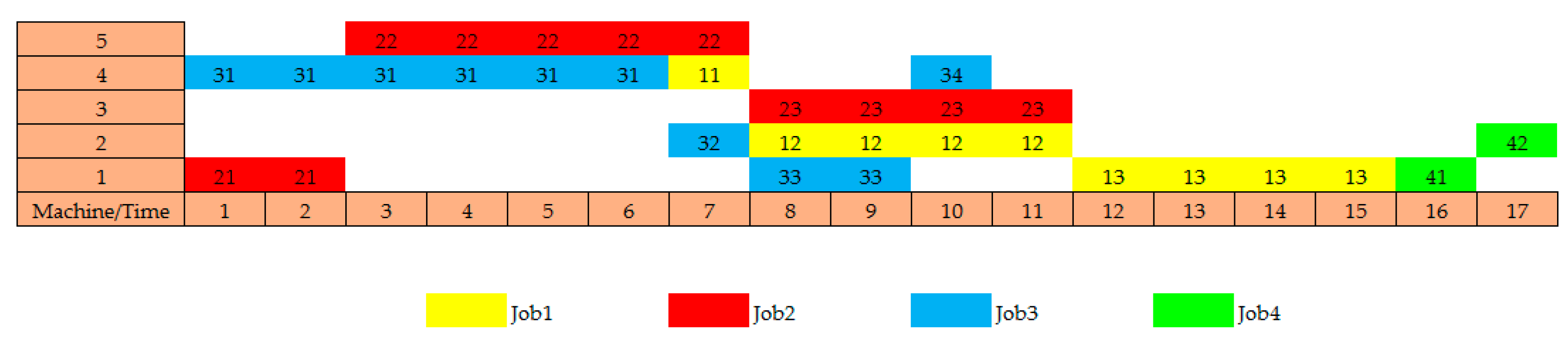
4.1.2. Procedure of FJSP by Using the Improved Differential Evolution Algorithm

(1) The improved DE was developed by applying four mutation equations [28], DE/rand-to-best/1/bin, DE/rand/2/bin, DE/rand/1/exp 2 position, and DE/best/2/exp 2 position, as seen in Equations (22), (23), (24), and (25), as follows:

$$V_{m,n,G}=X_{r1,n,G}+F1\left(X_{r2,n,G}-X_{r3,n,G}\right)+F2\left(X_{best,n,G}-X_{r1,n,G}\right)$$

(22)

$$V_{m,n,G}=X_{r1,n,G}+F\left(X_{r2,n,G}-X_{r3,n,G}+X_{r4,n,G}-X_{r5,n,G}\right)$$

(23)

$$V_{m,n,G}=X_{r1,n,G}+F\left(X_{r2,n,G}-X_{r3,n,G}+X_{r4,n,G}-X_{r5,n,G}\right)$$

(24)

$$V_{m,n,G}=X_{best,n,G}+F\left(X_{r2,n,G}-X_{r3,n,G}+X_{r4,n,G}-X_{r5,n,G}\right)$$

(25)

Let r1, r2, r3, r4, and r5 denote the vectors which are randomly selected from a set of target vectors j, which represents the best vector found so far in the algorithm. F is a predefined integer parameter (scaling factor). In the proposed heuristics, F is set to 2; i is the vector number which ranges from 1 to NP, and j is the position of a vector which runs from 1 to D.

(2) The improved DE was developed by applying one crossover or recombination equation at exponential crossover position 2, as seen in Equation (26) [29], as follows:

$$U_{i,j,G}=\{\begin{array}{c}{V}_{i,j,G} when j \le ran{d}_{i,1} and j \ge ran{d}_{i,2}\\ X_{i,j,G} when ran{d}_{i,1} < j < ran{d}_{i,2}\end{array}$$

(26)

As the predefined parameters in the proposed heuristics, let $rand{b}_i$ be a random number between 0 and 1 and let CR be the recombination probability. $rand{b}_i$, $rand{b}_{i,1},$ and $rand{b}_{i,2}$ are random integer numbers which represent the position of a vector; these random numbers range from 1 to D.

On the basis of the explanations in steps 1–4, the improved DE is shown in Algorithm 1.

Algorithm 1. Pseudo-code of the improved DE for the FJSP

Setup the initial DE parameter Do while from first iteration to final iteration  Do while from first DE to final DE   Setup the initial parameters: job, operation, machine, processing time,   operation sequence, machine assignment.   Do while from first task to final task    Find the start/following task where the fitness is the makespan of the data instances    Input the scaling factor, crossover rate, NP, job assignment, machine assignment, and    local search to data list    Produce the four mutation equations: $${\mathrm{V}}_{\mathrm{m},\mathrm{n},\mathrm{G}}={\mathrm{X}}_{\mathrm{r}1,\mathrm{n},\mathrm{G}}+\mathrm{F}1\left({\mathrm{X}}_{\mathrm{r}2,\mathrm{n},\mathrm{G}}-{\mathrm{X}}_{\mathrm{r}3,\mathrm{n},\mathrm{G}}\right)+\mathrm{F}2\left({\mathrm{X}}_{\mathrm{best},\mathrm{n},\mathrm{G}}-{\mathrm{X}}_{\mathrm{r}1,\mathrm{n},\mathrm{G}}\right)$$ $${\mathrm{V}}_{\mathrm{m},\mathrm{n},\mathrm{G}}={\mathrm{X}}_{\mathrm{r}1,\mathrm{n},\mathrm{G}}+\mathrm{F}\left({\mathrm{X}}_{\mathrm{r}2,\mathrm{n},\mathrm{G}}-{\mathrm{X}}_{\mathrm{r}3,\mathrm{n},\mathrm{G}}+{\mathrm{X}}_{\mathrm{r}4,\mathrm{n},\mathrm{G}}-{\mathrm{X}}_{\mathrm{r}5,\mathrm{n},\mathrm{G}}\right)$$ $${\mathrm{V}}_{\mathrm{m},\mathrm{n},\mathrm{G}}={\mathrm{X}}_{\mathrm{r}1,\mathrm{n},\mathrm{G}}+\mathrm{F}\left({\mathrm{X}}_{\mathrm{r}2,\mathrm{n},\mathrm{G}}-{\mathrm{X}}_{\mathrm{r}3,\mathrm{n},\mathrm{G}}+{\mathrm{X}}_{\mathrm{r}4,\mathrm{n},\mathrm{G}}-{\mathrm{X}}_{\mathrm{r}5,\mathrm{n},\mathrm{G}}\right)$$ $${\mathrm{V}}_{\mathrm{m},\mathrm{n},\mathrm{G}}={\mathrm{X}}_{\mathrm{best},\mathrm{n},\mathrm{G}}+\mathrm{F}\left({\mathrm{X}}_{\mathrm{r}2,\mathrm{n},\mathrm{G}}-{\mathrm{X}}_{\mathrm{r}3,\mathrm{n},\mathrm{G}}+{\mathrm{X}}_{\mathrm{r}4,\mathrm{n},\mathrm{G}}-{\mathrm{X}}_{\mathrm{r}5,\mathrm{n},\mathrm{G}}\right)$$    Developed by applying the two crossover or recombination equations: $${\mathrm{U}}_{\mathrm{i},\mathrm{j},\mathrm{G}}=\{\begin{array}{c}{\mathrm{V}}_{\mathrm{i},\mathrm{j},\mathrm{G}} \mathrm{when} \mathrm{j}\le {\mathrm{rand}}_{\mathrm{i},1} \mathrm{and} j \ge {\mathrm{rand}}_{\mathrm{i},2}\\ {\mathrm{X}}_{\mathrm{i},\mathrm{j},\mathrm{G}} \mathrm{when} {\mathrm{rand}}_{\mathrm{i},1} < j < {\mathrm{rand}}_{\mathrm{i},2}\end{array}.$$    Produce the new target vector (selection/process): $${\mathrm{X}}_{\mathrm{m},\mathrm{n},\mathrm{G}+1}=\{\begin{array}{c}{\mathrm{U}}_{\mathrm{m},\mathrm{n},\mathrm{G}} \mathrm{i}\mathrm{f} \mathrm{f}\left({\mathrm{U}}_{\mathrm{m},\mathrm{n},\mathrm{G}}\right)\le \mathrm{f}\left({\mathrm{X}}_{\mathrm{m},\mathrm{n},\mathrm{G}}\right)\\ {\mathrm{X}}_{\mathrm{m},\mathrm{n},\mathrm{G}},\mathrm{else}\end{array}.$$   End do  End do  Select the best solution from all DEs in the iteration End do Show/select the best solution from all DEs in all iterations

4.1.3. Procedure of FJSP by the Using Local Search with the Jump Search

The flexible job shop scheduling problem points to the optimal target of the minimum makespan. Considering the pathway of any latest complete operation, it denotes the critical pathway for flexible job shop scheduling. As shown in Figure 5 and Figure 6, the critical pathway is S → O_2,1 → O_4,1 → O_4,2 → O_4,3 → O_2,2 → O_2,3 → O_2,4 → T.

Figure 6 reveal the critical pathway for flexible job shop scheduling. This pathway is able to determine solutions using the local search and jump search methods through an algorithm that identifies target values from the sorted critical pathway by thoroughly checking any operation on the critical pathway. In Figure 6, operation O_2,1 is checked for possible intervention by a predecessor under these circumstances and priorities with a lower processing time and compatibility with an operating machine. Accordingly, operations are checked in the following consecutive order O_4,1 → O_4,2 → O_4,3 → O_2,2 → O_2,3 → O_2,4. Then, the fitness value is calculated in each round until completion of a set number of iterations.

5. Analysis of the Results from the Experiment on DE for Solving FJSP

To solve the flexible job shop scheduling problem, the Matlab program running on a personal computer (Core i5, 2.5 GHz, 8.00 GB RAM, Windows 7 operating system) was applied. It was developed by metaheuristic algorithms for the solutions focusing on the makespan.

Calculation factors were derived from the experiment based on optimization and relevant research. The findings were as follows: NP = 150, Iterate = 200, F = 2, CR = 0.8, number of iterated local search = 500 rounds. Moreover, the operation sequence that gave priority to operating the most remaining operations as well as machine assignment by choosing a machine with the minimum workload (MWL) were determined.

5.1. Results of Solving the Flexible Job Shop Scheduling Problem with Sample Problems from Kacem et al.

The results of solving the flexible job shop scheduling problem with sample problems from Kacem et al. [26,27] are shown in

Table 14. Summary of solving the flexible job shop scheduling problem with sample problems from Kacem et al. [26,27].

Problem	BKS	Mutation Strategy
		DE *	DE **	DE ***	DE ****
K01	11	12 (9.09)	12 (9.09)	11 (0.00)	11 (0.00)
K02	14	15 (7.14)	15 (7.14)	15 (7.14)	15 (7.14)
K03	11	11 (0.00)	11 (0.00)	11 (0.00)	11 (0.00)
K04	7	7 (0.00)	7 (0.00)	7 (0.00)	7 (0.00)
K05	11	12 (9.09)	12 (9.09)	12 (9.09)	12 (9.09)
MRE		5.06	5.06	3.25	3.25

* DE/rand to best/1/Bin; ** DE/rand/2/Bin; *** DE/rand/1/Exp Crossover Position 2/Local Search with Jump Search; **** DE/best/2/Exp Crossover Position 2/Local Search with Jump Search; Mean relative error (MRE); Best known solution (BKS).

, and a Gantt chart of solutions to problem K01 is shown in Figure 7.

In Table 14, the result of solving the flexible job shop scheduling problem with small size problems [26,27] is revealed. The solutions optimizing differential evolution algorithms that provide the most optimal solutions are a combination of DE/rand/1 and exponential position 2 as well as a combination of DE/best/2 and exponential position 2, resulting in a makespan of 11. These solutions are illustrated in the Gantt chart in Figure 7 for problem K01. A further finding is that the lowest MRE is 3.25.

5.2. Results of Solving the Flexible Job Shop Scheduling Problem with Sample Problems of Brandimarte

The results of solving the flexible job shop scheduling problem with the sample problems of Brandimarte [30] can be found in

Table 15. Summary of solving the flexible job shop scheduling problem with sample problems Brandimarte [30].

Problem	BKS	Mutation Strategy
		DE *	DE **	DE ***	DE ****
Mk1	40	43 (7.50)	43 (7.50)	40 (0.00)	40 (0.00)
Mk2	27	28 (7.69)	28 (7.69)	28 (7.69)	28 (7.69)
Mk3	204	204 (0.00)	204 (0.00)	204 (0.00)	204 (0.00)
Mk4	60	71 (18.33)	71 (18.33)	71 (18.33)	71 (18.33)
Mk5	174	178 (2.30)	178 (2.30)	179 (2.87)	179 (2.87)
Mk6	59	73 (23.73)	73 (23.73)	73 (23.73)	73 (23.73)
Mk7	143	149 (4.20)	149 (4.20)	148 (3.50)	146 (2.10)
Mk8	523	528 (0.96)	528 (0.96)	528 (0.96)	528 (0.96)
Mk9	307	324 (5.54)	321 (4.56)	323 (5.21)	321 (4.56)
Mk10	212	234 (10.38)	233 (9.90)	236 (11.32)	235 (10.85)
MRE		8.06	7.92	7.36	7.11

* DE/rand to best/1/Bin; ** DE/rand/2/Bin; *** DE/rand/1/Exp Crossover Position 2/Local Search with Jump Search; **** DE/best/2/Exp Crossover Position 2/Local Search with Jump Search; Mean relative error (MRE).

and the Gantt chart of solutions for problem Mk1 (Figure 8).

Table 15 shows the results of solving the flexible job shop scheduling problem for medium size problems using the sample problems of Brandimarte [30]. The solution optimizing the differential evolution algorithm that provides the most optimal solution is DE/best/2 combined with exponential position 2 and DE/rand/1 combined with exponential position 2, which results in a makespan of 40 and 204. This value is equal to the BKS value of the data set from sample Mk1 and Mk3. Furthermore, the lowest MRE value obtained is 7.11, as shown in the Gantt chart in Figure 8.

5.3. Results of Solving the Flexible Job Shop Scheduling Problem with Sample Problems of Dauzere-Peres and Paulli

The results of solving the flexible job shop scheduling problem with the sample problems of Dauzere-Peres and Paulli [31] can be found in

Table 16. Summary of solving the flexible job shop scheduling problem with sample problems Dauzere-Peres and Paulli.

Problem	BKS	Mutation Strategy
		DE *	DE **	DE ***	DE ****
01a	2530	2895 (14.42)	2750 (8.70)	2615 (3.36)	2645 (4.55)
04a	2555	2859 (11.90)	2770 (8.41)	2650 (3.72)	2610 (2.15)
07a	2396	2759 (15.15)	2650 (10.60)	2650 (10.60)	2510 (4.76)
09a	2074	2281 (9.98)	2269 (9.40)	2210 (6.56)	2150 (3.66)
11a	2078	2378 (14.44)	2366 (13.86)	2221 (6.88)	2200 (5.87)
MRE		13.18	10.19	6.22	4.20

* DE/rand to best/1/Bin; ** DE/rand/2/Bin; *** DE/rand/1/Exp Crossover Position 2/Local Search with Jump Search; **** DE/best/2/Exp Crossover Position 2/Local Search with Jump Search; Mean relative error (MRE).

.

Table 16 shows the results of solving the flexible job shop scheduling problem for large size problems using the sample problems of Dauzere-Peres and Paulli [31]. The solution optimizing the differential evolution algorithm that provides the best solution is DE/best/2 combined with exponential position 2, which results in a makespan of 2610. When compared with the other DE algorithm, it obtained the lowest value that is 4.20.

6. The Results of the Comparison of the DE Algorithm with Other Metaheuristic Methods

6.1. Results of Solving the Flexible Job Shop Scheduling Problem with Sample Problems of Brandimarte

A comparison of the differential evolution algorithm with other metaheuristic algorithms, GA and PSO, for the 10 comparative sample problems of Brandimarte [30] is given in

Table 17. Summary of comparing the differential evolution algorithm with other metaheuristic algorithms.

Problem	n × m × k *	BKS **	Chen et al. (GA) [32]	Girish and Jawahar (PSO) [33]	DE-FJSP
		Cmax	Cmax	Cmax	Cmax
Mk01	10 × 6 × 55	40	40 (0.00)	40 (0.00)	40 (0.00)
Mk02	10 × 6 × 58	27	29 (6.89)	27 (0.00)	28 (7.69)
Mk03	15 × 8 × 150	204	204 (0.00)	204 (0.00)	204 (0.00)
Mk04	15 × 8 × 90	60	63 (4.76)	62 (3.22)	71 (18.33)
Mk05	15 × 4 × 106	174	181 (3.86)	178 (2.24)	179 (2.87)
Mk06	10 × 15 × 150	59	60 (1.66)	78 (24.35)	73 (23.73)
Mk07	20 × 5 × 100	143	148 (3.38)	147 (2.72)	146 (2.10)
Mk08	20 × 10 × 225	523	523 (0.00)	523 (0.00)	528 (0.96)
Mk09	20 × 10 × 240	307	308 (0.32)	341 (9.97)	321 (4.56)
Mk10	20 × 15 × 240	212	212 (0.00)	252 (15.07)	235 (10.85)
MRE			2.08	7.75	7.11

* n = Job, m = Machine, k = Operation; ** Best known solution (BKS) ; FJSP = Flexible job shop scheduling problem; GA = Genetic algorithm; PSO = Particle swarm optimization.

.

Table 17 shows the comparative results for solving the flexible job shop scheduling problem using the differential evolution algorithm versus various dimension-optimizing algorithms. The value of mean of relative error (MRE) is lower than the value obtained by Girish and Jawahar [33] with PSO (7.75), while the improved DE has a value of 7.11. The work by Chen et al. [32] showed a value of 2.08 with the, while DE provided a greater value of 7.11. However, some problems, including Mk1 and Mk3, resulted in an equally good makespan in comparison with the BKS value of the data set.

6.2. Results of Solving the Flexible Job Shop Scheduling Problem with Sample Problems of Dauzere-Peres and Paulli

A comparison of the differential evolution algorithm with other metaheuristic algorithms, 1ST-DE, for the 5 comparative sample problems of Dauzere-Peres and Paulli [31] is given in

Table 18. Summary of comparing the differential evolution algorithm with other metaheuristic algorithms.

Problem	n × m × k *	BKS **	Wisittipanich (1ST-DE) [12]	DE-FJSP
		Cmax	Cmax	Cmax
01a	10 × 5 × 196	2530	2645 (4.55)	2645 (4.55)
04a	10 × 5 × 196	2555	2616 (2.39)	2610 (2.15)
07a	15 × 8 × 293	2396	2582 (7.76)	2510 (4.76)
09a	15 × 8 × 293	2074	2153 (3.81)	2150 (3.66)
11a	15 × 8 × 293	2078	2221 (6.88)	2200 (5.87)
MRE			5.08	4.20

* n = Job, m = Machine, k = Operation; ** Best known solution (BKS); FJSP = Flexible job shop scheduling problem.

.

Table 18 shows the comparative results for solving the flexible job shop scheduling problem using the differential evolution algorithm versus various dimension-optimizing algorithms. The value of mean of relative error (MRE) is lower than the value obtained by Wisittipanich [12] with 1ST-DE (5.08), while the improved DE has a value of 4.20. From the computational results, we can see that the improved DE algorithms with jump search are effective methods when compare with the basic DE and some meta-heuristic method.

7. Conclusions and Suggestions

This section presents the conclusions of this study. The differential evolution algorithm was used to solve the flexible job shop scheduling problem and optimize the dimensions. Among sample problems, the makespan and the BKS value of the data set were compared and the mean of relative error (MRE) was calculated. The sample problems of Kacem et al. were used as examples of small-sized problems. The dimensions were optimized by using “DE/rand/1” combined with exponential crossover position 2, as well as “DE/best/2” combined with exponential crossover position 2, which resulted in the minimum MRE value of 3.25. The sample problems of Brandimarte were used as examples of medium-sized problems. The dimensions were optimized with the combination of “DE/best/2” and exponential crossover position 2, providing a minimized MRE value of 7.11. Furthermore, the sample problems of Dauzere-Peres and Paulli were used as examples of large-sized problems. The dimensions were optimized with the combination of “DE/best/2” and exponential crossover position 2, providing a minimized MRE value of 4.20. Hence, the improved differential evolution in this research was able to solve the flexible job shop scheduling problem.

The DE algorithm proposed in this study can be applied to solve problems in the manufacturing industry in Thailand, such as mold and die manufacturing, the flexible job shop scheduling problem of the work center (FJSSPWC), or flexible job shop scheduling problem with preventive maintenance of the machine.

References

1. Karthikeyan, S.; Asokan, P.; Nickolas, S. A hybrid discrete firefly algorithm for multi-objective flexible job shop scheduling problem with limited resource constraints. Int. J. Adv. Manuf. Technol. 2014, 72, 1567–1579. [Google Scholar] [CrossRef]
2. Storn, R.; Price, K. Differential evolution—A simple and efficient heuristic for global optimization over continuous space. J. Glob. Optim. 1997, 11, 341–359. [Google Scholar] [CrossRef]
3. Xia, W.; Wu, Z. An effective hybrid optimization approach for multi-objective flexible job-shop scheduling problems. Comput. Ind. Eng. 2005, 48, 409–425. [Google Scholar] [CrossRef]
4. Kanate, P. Algorithm Development for Solving Flexible Job Shop Scheduling Problem. Ph.D. Thesis, Kasetsart University, Krung Thep Maha Nakhon, Thailand, 2011. [Google Scholar]
5. Tang, J.; Zhang, G.; Lin, B.; Zhang, B. A Hybrid Algorithm for Flexible Job-shop Scheduling Problem. Procedia Eng. 2011, 15, 3678–3683. [Google Scholar] [CrossRef]
6. Wannaporn, T.; Arit, T. Modified Genetic Algorithm for Flexible Job-Shop Scheduling Problems. Procedia Comput. Sci. 2012, 12, 122–128. [Google Scholar] [Green Version]
7. Thanyapon, U.; Pupong, P.; Kwanniti, K. Solving an Advanced Planning and Scheduling Problem with Preventive Maintenance Time Window Constraints by Mixed Integer Programming Models. Thai J. Oper. Res. 2016, 4, 1–15. Available online: https://www.tci-thaijo.org/index.php/TJOR/article/view/60994 (accessed on 22 July 2019).
8. Hamid, A.; Christoph, H.; Michael, D. Machine scheduling in production: A content analysis. Appl. Math. Model. 2017, 50, 279–299. [Google Scholar]
9. Li, X.; Gao, L. An Effective Hybrid Genetic Algorithm and Tabu Search for Flexible Job Shop Scheduling Problem. Int. J. Prod. Econ. 2016, 174, 93–110. [Google Scholar] [CrossRef]
10. Luan, F.; Cai, Z.; Wu, S.; Jiang, T.; Li, F.; Yang, J. Improved Whale Algorithm for Solving the Flexible Job Shop Scheduling Problem. Mathematics 2019, 7, 384. [Google Scholar] [CrossRef]
11. Li, X.; Peng, Z.; Du, B.; Guo, J.; Xu, W.; Zhuang, K. Hybrid artificial bee colony algorithm with a rescheduling strategy for solving flexible job shop scheduling problems. Comput. Ind. Eng. 2017, 113, 10–26. [Google Scholar] [CrossRef]
12. Wisittipanich, W. Minimizing Makespan in Flexible Job Shop Problems by Adapting the Differential Evolution. Thai J. Oper. Res. 2015, 3, 40–50. [Google Scholar]
13. Yuan, Y.; Xu, H. Flexible job shop scheduling using hybrid differential evolution algorithms. Comput. Ind. Eng. 2013, 65, 246–260. [Google Scholar] [CrossRef]
14. Bhaskara, P.; Padmanabhan, G.; Satheesh, K.B. Differential Evolution Algorithm for Flexible Job Shop Scheduling Problem. Int. J. Adv. Prod. Mech. Eng. 2015, 5, 71–79. [Google Scholar]
15. Wang, L.; Pan, Q.K.; Tasgetiren, M.F. Minimizing the total flow time in a flow shop with blocking by using hybrid harmony search algorithms. Expert Syst. Appl. 2010, 37, 7929–7936. [Google Scholar] [CrossRef]
16. Zhang, R.; Song, S.; Wu, C. A hybrid differential evolution algorithm for job shop scheduling problems with expected total tardiness criterion. Appl. Soft Comput. 2013, 13, 1448–1458. [Google Scholar] [CrossRef]
17. Cao, E.; Lai, M. The open vehicle routing problem with fuzzy demands. Expert Syst. Appl. 2010, 37, 15. [Google Scholar] [CrossRef]
18. Lai, M.; Cao, E. An improved differential evolution algorithm for vehicle routing problem with simultaneous pickups and deliveries and time windows. Eng. Appl. Artif. Intell. 2010, 23, 188–195. [Google Scholar]
19. Xu, H.; Wen, J. Differential Evolution Algorithm for the Optimization of the Vehicle Routing Problem in Logistics. In Proceedings of the 2012 Eighth International Conference on Computational Intelligence and Security, Guangzhou, China, 17–18 November 2012; pp. 48–51. [Google Scholar]
20. Cruz, I.L.; van Willigenburg, L.G.; van Straten, G. Efficient differential evolution algorithms for multimodal optimal control problems. Appl. Soft Comput. 2003, 3, 97–122. [Google Scholar] [CrossRef]
21. Adeyemo, J.; Otieno, F. Differential evolution algorithm for solving multi-objective crop planning model. Agric. Water Manag. 2010, 97, 848–856. [Google Scholar] [CrossRef]
22. Abou El Ela, A.A.; Abido, M.A.; Spea, S.R. Optimal power flow using differential Evolution algorithm. Electr. Power Syst. Res. 2010, 80, 878–885. [Google Scholar] [CrossRef]
23. Kuila, P.; Jana, P.K. A novel differential evolution based clustering Algorithm for wireless sensor networks. Appl. Soft Comput. 2014, 25, 414–425. [Google Scholar] [CrossRef]
24. Sharma, S.; Rangaiah, G.P. An improved multi-objective differential evolution with a termination criterion for optimizing chemical processes. Comput. Chem. Eng. 2013, 56, 155–173. [Google Scholar] [CrossRef]
25. Pitakaso, R.; Parawech, P.; Jirasirierd, G. Comparisons of Different Mutation and Recombination Processes of the DEA for SALB-1. In Proceedings of the Institute of Industrial Engineers Asian Conference, Taipei, Taiwan, 18–20 July 2013; pp. 1571–1579. [Google Scholar]
26. Kacem, I.; Hammadi, S.; Borne, P. Approach by localization and multiobjective evolutionary optimization for flexible job-shop scheduling problems. IEEE Trans. Syst. Man Cybern. 2002, 32, 1–13. [Google Scholar] [CrossRef]
27. Kacem, I.; Hammadi, S.; Borne, P. Pareto-optimality approach for flexible job-shop scheduling problems: hybridization of evolutionary algorithms and fuzzy logic. Math. Comput. Simul. 2002, 60, 245–276. [Google Scholar] [CrossRef]
28. Nguyen, S.; Kitchitvichynukul, V.; Wisittipanich, W. ET-Lib User’s Guide. Volume 2. Differential Evolution; Asian Institute of Technology: Khlong Luang, Thailand, 2013. [Google Scholar]
29. Poontana, S.; Nuchsara, K.; Preecha, K.; Krit, C. U-Shaped Assembly Line Balancing by Using Differential Evolution Algorithm. Math. Comput. Appl. 2018, 23, 79. [Google Scholar] [Green Version]
30. Brandimarte, P. Routing and Scheduling in a Flexible Job Shop by Tabu Search. Ann. Oper. Res. 1993, 41, 157–183. [Google Scholar] [CrossRef]
31. Dauzere-Peres, S.; Paulli, J. An integrated approach for modeling and solving the general multiprocessor job-shop scheduling problem using tabu search. Ann. Oper. Res. 1997, 70, 281–306. [Google Scholar] [CrossRef]
32. Chen, H.; Ihlow, J.; Lehmann, C. A genetic algorithm for flexible job-shop scheduling. In Proceedings of the IEEE International Conference on Robotics and Automation, Detroit, MI, USA, 10–15 May 1999; pp. 1120–1125. [Google Scholar]
33. Girish, B.S.; Jawahar, N. A particle swarm optimization algorithm for flexible job shop scheduling problem. In Proceedings of the IEEE International Conference on Automation Science and Engineering, Bangalore, India, 22–25 August 2009; pp. 298–303. [Google Scholar]
Figure 1. Flexible job shop scheduling problem pattern.
Mca 24 00080 g001
Figure 2. Gantt chart of solutions.
Mca 24 00080 g002
Figure 3. General differential evolution algorithm procedure.
Mca 24 00080 g003
Figure 4. Gantt chart of sample problems.
Mca 24 00080 g004
Figure 5. Disjunction graph of flexible job shop scheduling.
Mca 24 00080 g005
Figure 6. Critical pathway for flexible job shop scheduling.
Mca 24 00080 g006
Figure 7. Gantt chart of solutions to flexible job shop scheduling problem K01 presented by Kacem et al. [26,27].
Mca 24 00080 g007
Figure 8. Gantt chart of solutions for flexible job shop scheduling problem Mk1 presented by Brandimarte [30].
Mca 24 00080 g008