2D Hybrid Steady-State Magnetic Field Model for Linear Induction Motors

Abstract

This paper presents a 2D hybrid steady-state magnetic field model, capable of accurately modeling the electromagnetic behavior in a linear induction motor, including primary slotting, finite yoke length, and longitudinal end-effects by primary motion. This model integrates a complex harmonic modeling technique with a discretized magnetic equivalent circuit model. The Fourier model is applied to regions with homogeneous material properties, e.g., air regions and the track of the motor, while the magnetic equivalent circuit (MEC) approach is used for the regions containing non-homogeneous material properties, e.g., the primary of the linear induction motor (LIM). By only meshing the domains containing highly-permeable materials, the computational effort is reduced in comparison with the finite element method (FEM). The model is applied to a double-layer single-sided LIM, and the resulting thrust and normal forces show an excellent agreement with respect to finite element analysis and measurement data.

1. Introduction

Linear induction motors (LIM) are widely used in long-stroke linear motion systems because of their inexpensive and robust construction. To obtain an optimal design, comprehensive methods able to predict the magnetic field distribution inside the electromagnetic structures play a crucial role. To allow extensive exploration of the design space, numerical methods such as the finite element method (FEM) are not preferable, as these models are computationally expensive.

In the literature, semi-analytical or hybrid methods are discussed, intending to reduce the needed computational efforts, while ensuring comparable accuracy to the numerical methods. However, all modeling techniques require certain assumptions, which limit their flexibility. In [1], an equivalent-circuit model of the LIM was proposed, determining the motor output thrust and vertical forces, while accounting for the longitudinal end-effects as a result of primary movement with respect to the secondary. In [2], an equivalent-circuit model for a high-speed industrial transportation LIM was presented, where the dynamic longitudinal and the transverse end-effects were accounted for by correction factors. In [3], an optimized end-effect equivalent-circuit model for LIM was presented, allowing modeling of partially-filled end-slots. However, equivalent circuit models are not suitable for design purposes, as their components need to be determined from measurements or magnetic field modeling [4].

In [5,6,7], magnetic field models for rotating and linear induction motors, using a two-dimensional field description by Fourier series, were presented. Although these models allow obtaining the magnetic field distribution inside the air gap, they do not include the magnetic field distribution inside the primary yoke or slots. In [5], the magnetic field distribution into a solid rotor was predicted, while considering the stator slots and tooth-tips and assuming an infinite permeability inside the stator yoke. In [6], the current carrying primary coils were replaced with infinitely-thin current sheets, and the primary slotting was accounted for by the use of Carter’s coefficient. In [7], correction factors for the longitudinal end-effect and also for the primary core losses were presented. A semi-analytical model for LIM, based on harmonic modeling, was presented in [8]. The field inside the primary slotting was calculated, assuming an infinitely-permeable core, but the longitudinal end-effects of the motor and the magnetic field distribution in the primary yoke were neglected.

In [9,10], the primary core of a synchronous permanent magnet motor was successfully included in the field analysis. In [11], these models were extended to include saturation of the highly-permeable materials. Hybrid models combine the benefits of the magnetic equivalent circuit (MEC) method [12] and harmonic modeling [13]. However, these models have only been derived for magnetostatic fields, thus neglecting eddy-current effects.

As an alternative to the aforementioned magnetostatic hybrid techniques, this study presents a steady-state hybrid semi-analytical model, which combines an MEC-based description of the domains containing highly-permeable materials, e.g., the primary of the LIM, with complex Fourier modeling applied to the conductive medium of the secondary plate and surrounding air regions. This model allows modeling of the full primary core of the LIM, including longitudinal end-effects and the electromagnetic field in the primary yoke and slotting, while also accounting for the primary velocity. Including the velocity terms to the field solution allows time-stepping to be avoided, thus saving time, when compared to FEA.

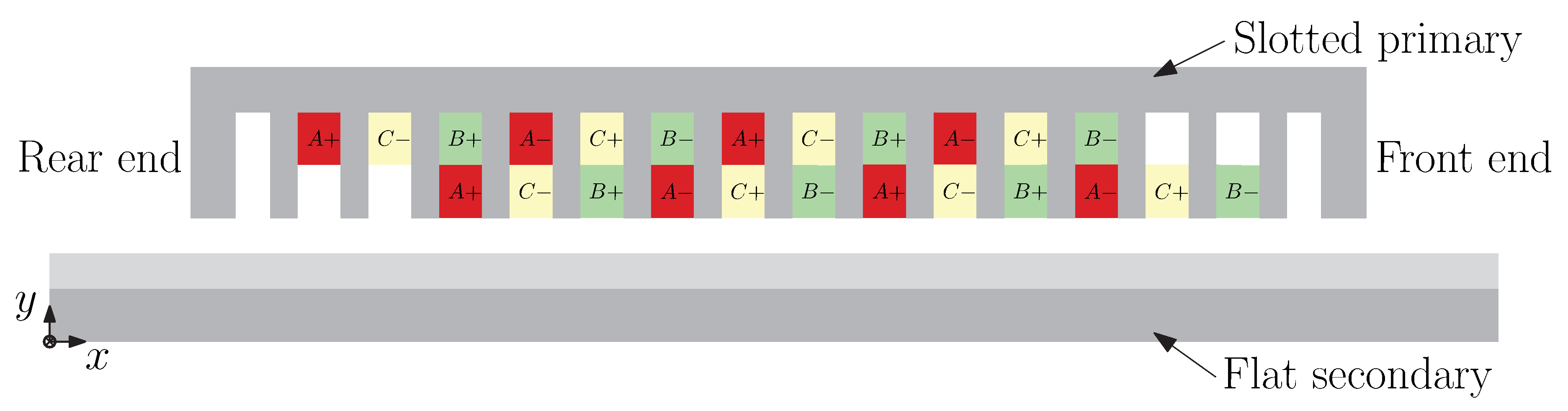
The electromagnetic problem that is investigated in this paper is a linear induction motor (LIM) topology with a moving primary and an infinitely-long flat secondary (Figure 1). The primary contains a rewound laminated core from a Tecnotion TL-15 linear synchronous permanent magnet motor with double-layer three-phase distributed winding [14]. This topology is used to validate the model with static measurements.

In this paper, a generalized description of the modeling methodology is presented in Section 2. Afterwards, the introduced model is applied to a double-layer single-sided LIM and validated with respect to a 2D steady-state FEA simulation and measurement data for the same topology, and the results are discussed in Section 3. Finally, the conclusions are presented in Section 4.

2. Modeling Methodology

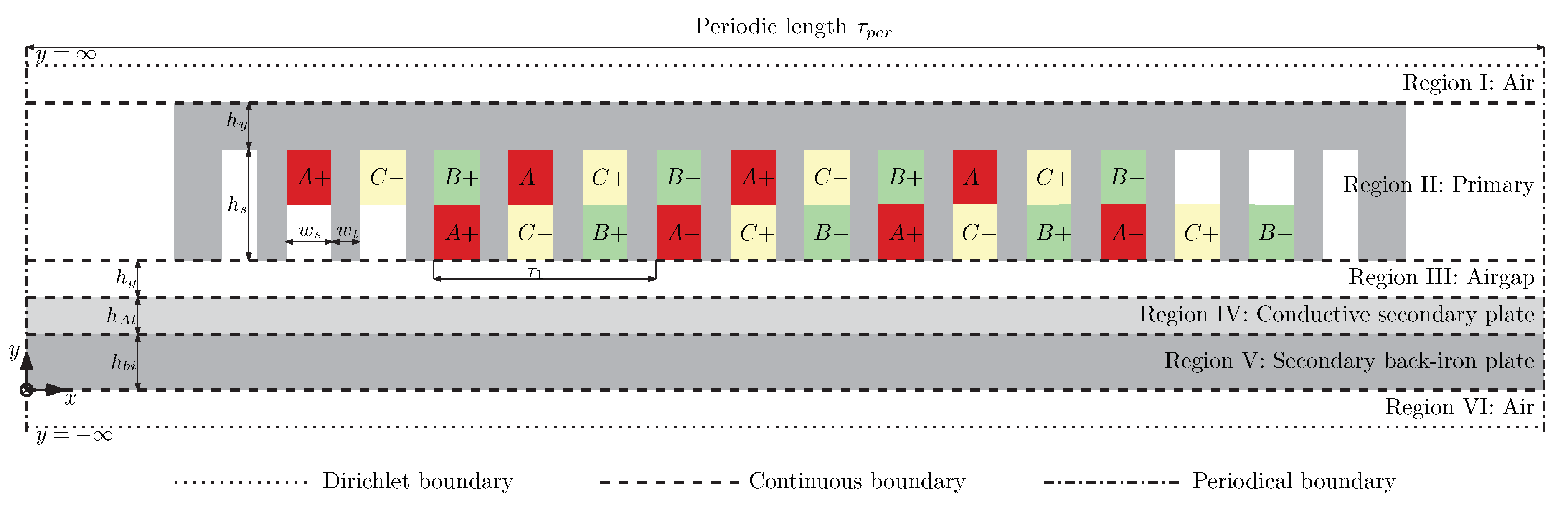
To apply the hybrid modeling technique to an electromagnetic problem like the LIM, the topology was represented in the 2D Cartesian coordinate system and is divided into orthogonal regions, as depicted in Figure 2. The complex harmonic modeling was applied to Regions I, III, IV, V, and VI, as these regions contained only homogeneous, isotropic, and linear materials. As the primary of the LIM (Region II) contained different materials along the x-direction and y-direction, it was modeled using the mesh-based MEC formulation. Using the complex harmonic formulation required periodicity in the longitudinal direction. As the secondary of the LIM was considered infinitely long, and the finite length of the primary was included in the analysis to account for the longitudinal end-effects, while the periodicity in x-direction was ensured by adding air at the front and rear end of the primary yoke, defining the periodical length ${\tau }_{per}$ for the whole problem.

The currents flowing into the three-phase distributed winding were as follows:

$$\begin{array}{ccc}\hfill I_{phA}(t)& =& I_p{e}^{j2\pi ft},\hfill \end{array}$$

(1)

$$\begin{array}{ccc}\hfill I_{phB}(t)& =& I_p{e}^{-j\frac{2\pi }{3}}{e}^{j2\pi ft},\hfill \end{array}$$

(2)

$$\begin{array}{ccc}\hfill I_{phC}(t)& =& I_p{e}^{j\frac{2\pi }{3}}{e}^{j2\pi ft},\hfill \end{array}$$

(3)

where f is the synchronous frequency, $I_p$ is the peak current, and t is the instance of time.

2.1. Complex Harmonic Modeling

The complex harmonic modeling technique is based on the analytical solution of the magnetic vector potential $A_z$, which was explained in detail in [15]. To derive the steady-state solution for the magnetic vector potential, time variation has to be included to account for the induced currents in the conductive regions. Their relation to the vector potential is expressed by the diffusion equation:

$$\begin{array}{c}\hfill \frac{{\partial }^2{A}_z}{\partial x^2}+\frac{{\partial }^2{A}_z}{\partial y^2}={\mu }_0{\mu }_r\sigma \frac{\partial A_z}{\partial t},\end{array}$$

(4)

where $\sigma$ is the conductivity of the considered region, ${\mu }_0$ is the relative permeability of the free space, and ${\mu }_r$ is the relative permeability of the material in that region. The general form of the solution to the magnetic vector potential is obtained in complex form:

$$\begin{array}{c}\hfill A_z(x,y,t)=\sum _{n=-\infty }^{\infty }(a_n{e}^{\sqrt{{\lambda }_n^2}y}+b_n{e}^{-\sqrt{{\lambda }_n^2}y})e^{j{\omega }_{n}x}{e}^{j(2\pi ft+{\omega }_{n}vt)},\end{array}$$

(5)

where:

$$\begin{array}{c}\hfill {\lambda }_n^2={\omega }_n^2+j{\mu }_0{\mu }_r\sigma (2\pi f+{\omega }_{n}v),\end{array}$$

(6)

$$\begin{array}{c}\hfill {\omega }_n=\frac{2n\pi }{{\tau }_{per}}.\end{array}$$

(7)

In (5), ${\omega }_n$ is the spatial frequency for the $n^{\mathrm{th}}$ space harmonic, v is the considered steady-state velocity of the primary with respect to the secondary, and $a_n$ and $b_n$ are the unknown coefficients for each harmonic, obtained from the applied boundary conditions explained in the following section.

The resulting flux density distributions for the tangential and normal direction were obtained as follows:

$$\begin{array}{c}\hfill B_x(x,y,t)=\frac{\partial A_z(x,y,t)}{\partial y}=\sum _{n=-\infty }^{\infty }\left[{\lambda }_n(a_n{e}^{{\lambda }_{n}y}-b_n{e}^{-{\lambda }_{n}y})\right]e^{j{\omega }_{n}x}{e}^{j(2\pi ft+{\omega }_{n}vt)},\end{array}$$

(8)

$$\begin{array}{c}\hfill B_y(x,y,t)=-\frac{\partial A_z(x,y,t)}{\partial x}=-j\sum _{n=-\infty }^{\infty }\left[{\omega }_n(a_n{e}^{{\lambda }_{n}y}+b_n{e}^{-{\lambda }_{n}y})\right]e^{j{\omega }_{n}x}{e}^{j(2\pi ft+{\omega }_{n}vt)}.\end{array}$$

(9)

2.2. MEC

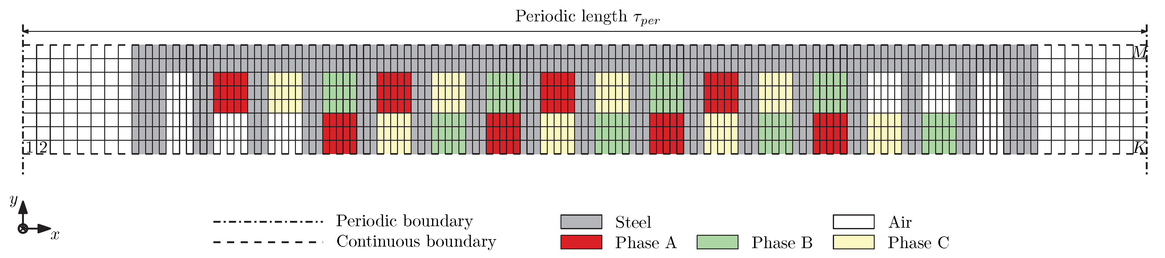
The primary of the LIM contained non-homogeneous material properties along the x- and y-direction, and for that reason, it was modeled using the MEC formulation. The region was discretized into L layers along the y-direction, each containing K rectangular elements along the x-direction, forming a mesh of $M=L\times K$ elements, as illustrated in Figure 3.

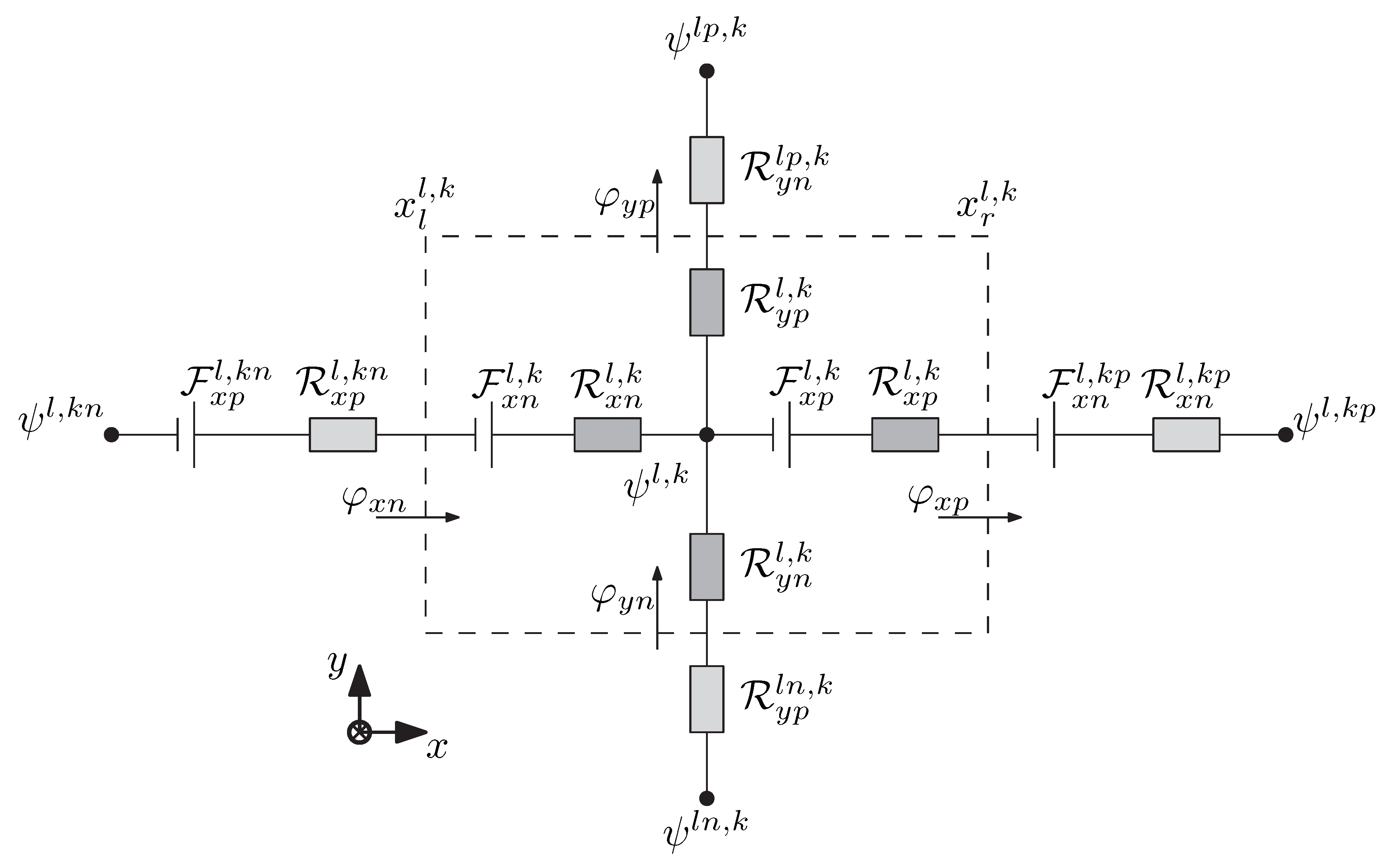
Each MEC-element encompassed one potential node, $\psi (l,k)$, as is shown in Figure 4, and time dependency was accounted for by adapting the following expression:

$$\begin{array}{c}\hfill \psi (l,k,t)=\psi (l,k)e^{j2\pi ft},\end{array}$$

(10)

where $\psi (l,k)$ is the complex value for each potential node, which is obtained after solving the set of linear equations, formed from the applied boundary conditions.

The reluctances for each MEC-element were defined by its dimensions and material properties:

$$\begin{array}{ccc}\hfill {\mathcal{R}}_{xp}(l,k)& =& {\mathcal{R}}_{xn}(l,k)=\frac{l_x(l,k)}{2{\mu }_0{\mu }_r(l,k)S_{zy}(l,k)},\hfill \end{array}$$

(11)

$$\begin{array}{ccc}\hfill {\mathcal{R}}_{yp}(l,k)& =& {\mathcal{R}}_{yn}(l,k)=\frac{l_y(l,k)}{2{\mu }_0{\mu }_r(l,k)S_{xz}(l,k)},\hfill \end{array}$$

(12)

where $l_x(l,k)$ and $l_y(l,k)$ are the lengths of each MEC-element in the x- and y-direction (Figure 4), $x_l^{l,k}$ and $x_r^{l,k}$ are the left and right coordinates of the MEC element, while $S_{zx}(l,k)$ and $S_{yz}(l,k)$ are the cross-sectional areas parallel to the $zx$- and $yz$-planes, respectively. The values, assigned to ${\mu }_r$, depend on each element’s location in the $xy$-plane, and as a consequence, the material each element encloses.

The magnetic equivalence of Kirchoff’s current law was applied to each MEC-element. All magnetic flux entering one potential node ($\psi (l,k,t)$) should be equal to the magnetic flux leaving this node:

$$\begin{array}{c}\hfill {\phi }_{xn}(l,k,t)+{\phi }_{yn}(l,k,t)={\phi }_{xp}(l,k,t)+{\phi }_{yp}(l,k,t),\end{array}$$

(13)

where:

$$\begin{array}{ccc}\hfill {\phi }_{xp}(l,k,t)& =& \frac{\psi (l,kp,t)-\psi (l,k,t)}{{\mathcal{R}}_{xp}(l,k)+{\mathcal{R}}_{xn}(l,kp)}+\frac{{\mathcal{F}}_{xp}(l,k,t)+{\mathcal{F}}_{xn}(l,kp,t)}{{\mathcal{R}}_{xp}(l,k)+{\mathcal{R}}_{xn}(l,kp)},\hfill \end{array}$$

(14)

$$\begin{array}{ccc}\hfill {\phi }_{xn}(l,k,t)& =& \frac{\psi (l,k,t)-\psi (l,kn,t)}{{\mathcal{R}}_{xn}(l,k)+{\mathcal{R}}_{xp}(l,kn)}+\frac{{\mathcal{F}}_{xn}(l,k,t)+{\mathcal{F}}_{xp}(l,kn,t)}{{\mathcal{R}}_{xn}(l,k)+{\mathcal{R}}_{xp}(l,kn)},\hfill \end{array}$$

(15)

$$\begin{array}{ccc}\hfill {\phi }_{yp}(l,k,t)& =& \frac{\psi (lp,k,t)-\psi (l,k,t)}{{\mathcal{R}}_{yp}(l,k)+{\mathcal{R}}_{yn}(lp,k)},\hfill \end{array}$$

(16)

$$\begin{array}{ccc}\hfill {\phi }_{yn}(l,k,t)& =& \frac{\psi (l,k,t)-\psi (ln,k,t)}{{\mathcal{R}}_{yn}(l,k)+{\mathcal{R}}_{yp}(ln,k)},\hfill \end{array}$$

(17)

where $kp$, $kn$, $lp$, and $ln$ represent the indices of neighboring potential nodes.

To allow coupling with the complex harmonic regions, periodicity in the x-direction is fulfilled by linking the last element of each layer with the first element from the same layer.

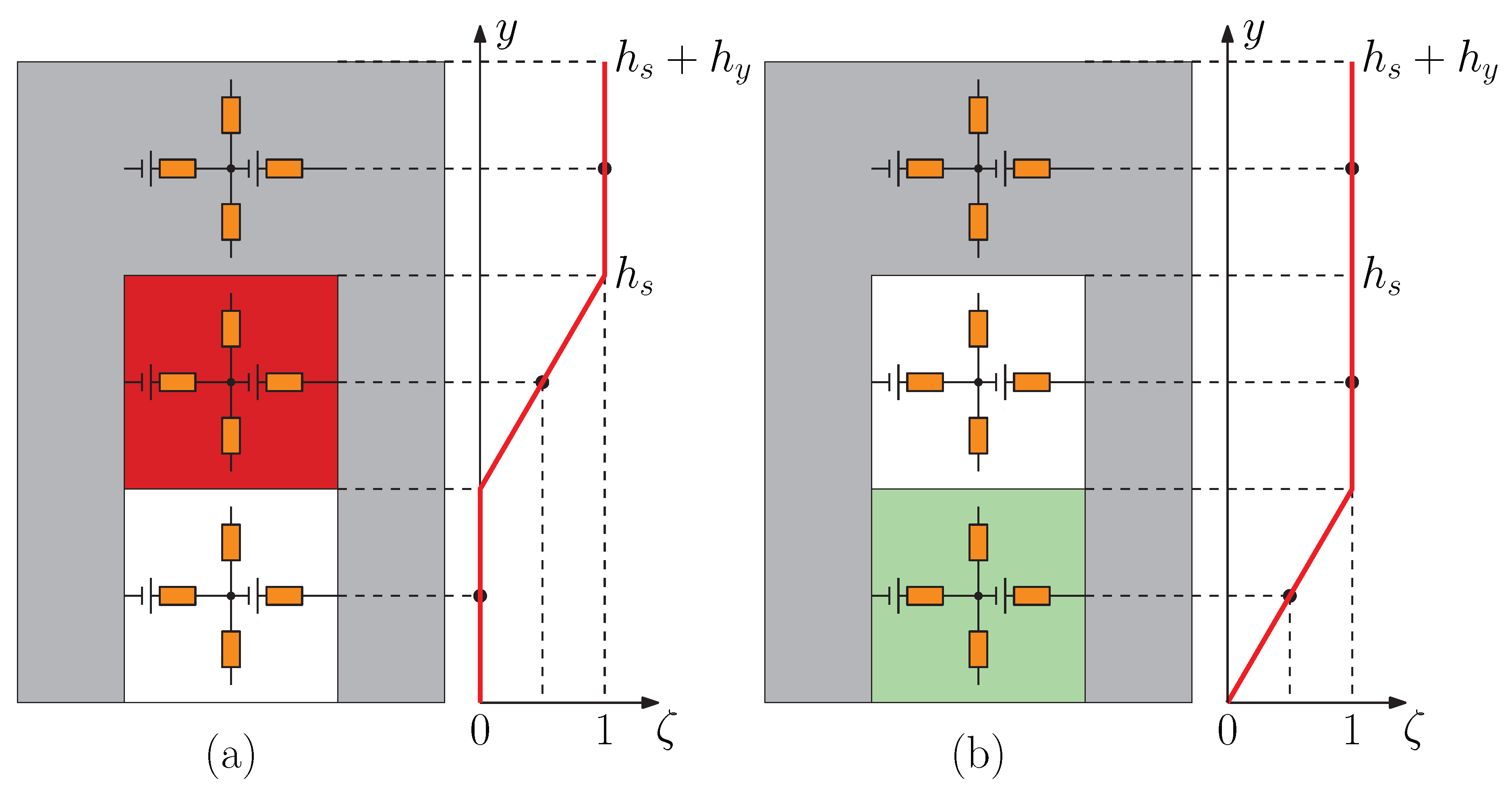
The MMFsource terms, present in the primary of the LIM, included only coil excitations represented by MMF-sources:

$$\begin{array}{ccc}\hfill {\mathcal{F}}_x(l,k,t)& =& \zeta \frac{N_t{I}_{ph}(t)}{2K_c},\hfill \end{array}$$

(18)

where $I_{ph}$ is the complex phase current according to (1)–(3), $N_t$ is the number of turns for a single coil, $K_c$ is the number of MEC elements in the x-direction for a single coil, and $\zeta$ represents the scaling factor to account for the distribution of the MMF sources along the y-direction. In Figure 5, the magnitude variation of the MMF-sources in the top and bottom layer coils is depicted. The magnitude was maximal in the yoke elements, as the formed magnetic path through the air gap enclosed the whole area of the coil, while in the slot elements, the magnitude of the MMF-sources was proportional to the enclosed coil area. In case coils were present in both layers, superposition of both MMF-sources was applied.

2.3. Boundary Conditions

To obtain the unknown coefficients for both harmonic and MEC regions, a set of linear equations, accounting the boundary conditions between every two adjacent regions, was solved. The presence of air above the primary and beneath the secondary of the investigated topology allowed the top and bottom boundaries of LIM to be extended to infinity, and thus, the Dirichlet boundary condition, forcing all field components to vanish, applied. To ensure continuity between every two neighboring Fourier regions i and j (e.g., Regions III and IV), the tangential components of the magnetic field strength and the normal components of the flux density, obtained by (8) and (9) for both regions, were equated. Analogically, the continuous boundary condition applied also on the border between each Fourier and MEC region (e.g., Regions I and II). While the obtained expressions for the magnetic fields in the harmonic regions were defined for the full periodical section of the analyzed problem, each expression for the MEC region was associated with a single mesh-element. A detailed explanation of the boundary conditions for both normal and tangential field components was given in [15], considering trigonometric harmonic solutions.

The main differences introduced by the complex harmonic solution, presented in this paper, were in the expressions of the coupled normal and tangential field components between each adjacent Fourier and MEC region.

Adapting (13), the coupled flux in the normal direction at the bottom and top of the MEC region took the form of:

$$\begin{array}{c}\hfill {\phi }_{xn}(1,k,t)+{\phi }_{yn}^{HM}(1,k,t)={\phi }_{xp}(1,k,t)+{\phi }_{yp}(1,k,t),\end{array}$$

(19)

$$\begin{array}{c}\hfill {\phi }_{xn}(L,k,t)+{\phi }_{yn}(L,k,t)={\phi }_{xp}(L,k,t)+{\phi }_{yp}^{HM}(L,k,t),\end{array}$$

(20)

where for the bottom layer of the MEC:

$$\begin{array}{ccc}\hfill {\phi }_{yn}^{HM}(1,k,t)& =& L_s\underset{x_l(1,k)-vt}{\overset{x_r(1,k)-vt}{\int }}{B}_y^{HM}(x,y_{BC})\mathrm{d}x,\hfill \\ & =& L_s\sum _{n=-\infty }^{\infty }(a_n{e}^{{\lambda }_n{y}_{BC}}+b_n{e}^{-{\lambda }_n{y}_{BC}})(e^{j{\omega }_n{x}_l(1,k)}-e^{j{\omega }_n{x}_r(1,k)})e^{j2\pi ft},\hfill \end{array}$$

(21)

for $1\le k\le K$, where $y_{BC}$ is the y-coordinate between the regions, to which the boundary condition applies, and $L_s$ is the depth of the domain. For the top layer of MEC, ${\phi }_{yp}^{HM}(L,k,t)$ was derived analogically.

Substituting the derived equation for $B_x$ from the adjacent Fourier region (8), the boundary condition for the tangential field strength used the the constitute relation $B={\mu }_0{\mu }_{r}H$ and took the form of:

$$\begin{array}{c}\hfill \frac{1}{{\mu }_0{\mu }_r^{HM}}{B}_x^{HM}(x,y_{BC},t)=\sum _{k=1}^K\frac{1}{{\mu }_0{\mu }_r^{MEC}(l,k)}{B}_x^{MEC}(x,y_{BC},t),\end{array}$$

(22)

where ${\mu }_r^{HM}$ represents the homogeneous relative permeability within the Fourier region, while ${\mu }_r^{MEC}(l,k)$ is the relative permeability per element of the MEC-region. The magnetic flux density, calculated for the top or bottom layer of the MEC-region, was considered to be constant within a single element [9]. To allow coupling with the neighboring Fourier regions, the right-hand side of (22) was modified as:

$$\begin{array}{c}\hfill B_x^{MEC}(x,y_{BC},t)=\sum _{n=-\infty }^{\infty }\frac{2}{{\tau }_{per}}\sum _{k=1}^K\underset{x_l(1,k)-vt}{\overset{x_r(1,k)-vt}{\int }}{B}_x^{MEC}(l,k,t)e^{-j{\omega }_{n}x}\mathrm{d}x,\end{array}$$

(23)

where:

$$\begin{array}{c}\hfill B_x^{MEC}(l,k,t)=\sum _{k=1}^K\frac{{\phi }_{xn}(l,k,t)+{\phi }_{xp}(l,k,t)}{2S_{zy}(l,k)}\end{array}$$

(24)

is the average tangential flux density per element and $l=L$ or $l=1$ for the top or bottom layer, respectively.

2.4. Force Calculation

The output thrust and normal forces acting on the primary were derived from the Maxwell stress tensor evaluated inside the air gap [16]. Taking into account the derived equations for $B_x$ and $B_y$ for Region III, the analytical force equations took the form of:

$$\begin{array}{c}\hfill F_x=-\frac{L_s}{{\mu }_0}\underset{0}{\overset{{\tau }_{per}}{\int }}\left[B_{xn}(x,y,t)B_{yn}^{*}(x,y,t)\right]dx\\ \hfill =-\frac{j{L}_s{\tau }_{per}}{2{\mu }_0}\sum _{n=-\infty }^{\infty }\left[{\lambda }_n{\omega }_n(a_n{e}^{{\lambda }_{n}y}-b_n{e}^{-{\lambda }_{n}y})(a_n^{*}{e}^{{\lambda }_n^{*}y}+b_n^{*}{e}^{-{\lambda }_n^{*}y})\right]\end{array}$$

(25)

and:

$$\begin{array}{c}\hfill F_y=-\frac{L_s}{2{\mu }_0}\underset{0}{\overset{{\tau }_{per}}{\int }}\left[B_{xn}(x,y,t)B_{xn}^{*}(x,y,t)-B_{yn}(x,y,t)B_{yn}^{*}(x,y,t)\right]dx\\ \hfill =-\frac{L_s{\tau }_{per}}{4{\mu }_0}\sum _{n=-\infty }^{\infty }[{\lambda }_n{\lambda }_n^{*}(a_n{e}^{{\lambda }_{n}y}-b_n{e}^{-{\lambda }_{n}y})(a_n^{*}{e}^{{\lambda }_n^{*}y}-b_n^{*}{e}^{-{\lambda }_n^{*}y})\\ \hfill -{\omega }_n^2(a_n{e}^{{\lambda }_{n}y}+b_n{e}^{-{\lambda }_{n}y})(a_n^{*}{e}^{{\lambda }_n^{*}y}+b_n^{*}{e}^{-{\lambda }_n^{*}y})],\end{array}$$

(26)

where * is the complex conjugate.

2.5. Joule Losses’ Calculation

The conduction losses inside the secondary can be calculated, using the Poynting vector, applied in the air gap (Region III) [17]:

$$\begin{array}{c}\hfill P_{joule,sec}=-\frac{L_s}{2}\Re \underset{0}{\overset{{\tau }_{per}}{\int }}{E}_z(x,y,t)H_x^{*}(x,y,t)dx\\ \hfill =-\frac{L_s{\tau }_{per}}{j2{\mu }_0}\sum _{n=-\infty }^{\infty }\left[({\lambda }_n^{*}\omega +{\lambda }_n^{*}{\omega }_{n}v)(a_n{e}^{{\lambda }_{n}y}+b_n{e}^{-{\lambda }_{n}y})(a_n^{*}{e}^{{\lambda }_n^{*}y}+b_n^{*}{e}^{-{\lambda }_n^{*}y})\right],\end{array}$$

(27)

where the following expressions were used:

$$\begin{array}{ccc}\hfill E_z(x,y,t)& =& -\frac{\partial A_z(x,y,t)}{\partial t},\hfill \end{array}$$

(28)

$$\begin{array}{ccc}\hfill H_x^{*}(x,y,t)& =& \frac{1}{{\mu }_0}{B}_x^{*}(x,y,t).\hfill \end{array}$$

(29)

3. Results and Model Validation

To validate the presented 2D complex hybrid steady-state model, 2D finite element analysis (FEA) was performed on the same topology.

Table 1. Parameters of the double-layer single-sided LIM.

Parameter	Symbol	Value	Unit
Number of phases	$N_p$	3	-
Number of poles	$2p$	6	-
Number of slots	$z_1$	16	-
Number of turns per coil	$N_t$	57	-
Stack width	$L_s$	50	mm
Fundamental pitch of the primary	${\tau }_1$	12	mm
Primary tooth width	$w_t$	6	mm
Primary slot width	$w_s$	10	mm
Primary slot height	$h_s$	20	mm
Primary yoke height	$h_y$	$6.5$	mm
Air gap length	$h_g$	$2.7$	mm
Thickness of the aluminum plate	$h_{Al}$	2	mm
Thickness of the back-iron plate	$h_{bi}$	8	mm
Conductivity of aluminum	${\sigma }_{Al}$	$17\times {10}^6$	Sm${}^{-1}$
Conductivity of iron	${\sigma }_{Fe}$	$4.5\times {10}^6$	Sm${}^{-1}$
Relative permeability iron	${\mu }_r$	1000	mm

contains the dimensions and design parameters used for both simulations. For the complex hybrid model, $N=100$ harmonics and $K=576$ elements in $L=53$ layers were used, in order to generate a dense enough mesh, able to model the magnetic field in the primary of the motor and in the surrounding air accurately. The periodic length ${\tau }_{per}$ for both the complex hybrid model and FEA was selected to be even times the fundamental pitch of one periodical section of the primary ${\tau }_1$ (in this case, ${\tau }_{per}=12\times {\tau }_1$). The conductivity of the aluminum plate was reduced accordingly, to take into consideration the transverse end-effects of the investigated motor [18].

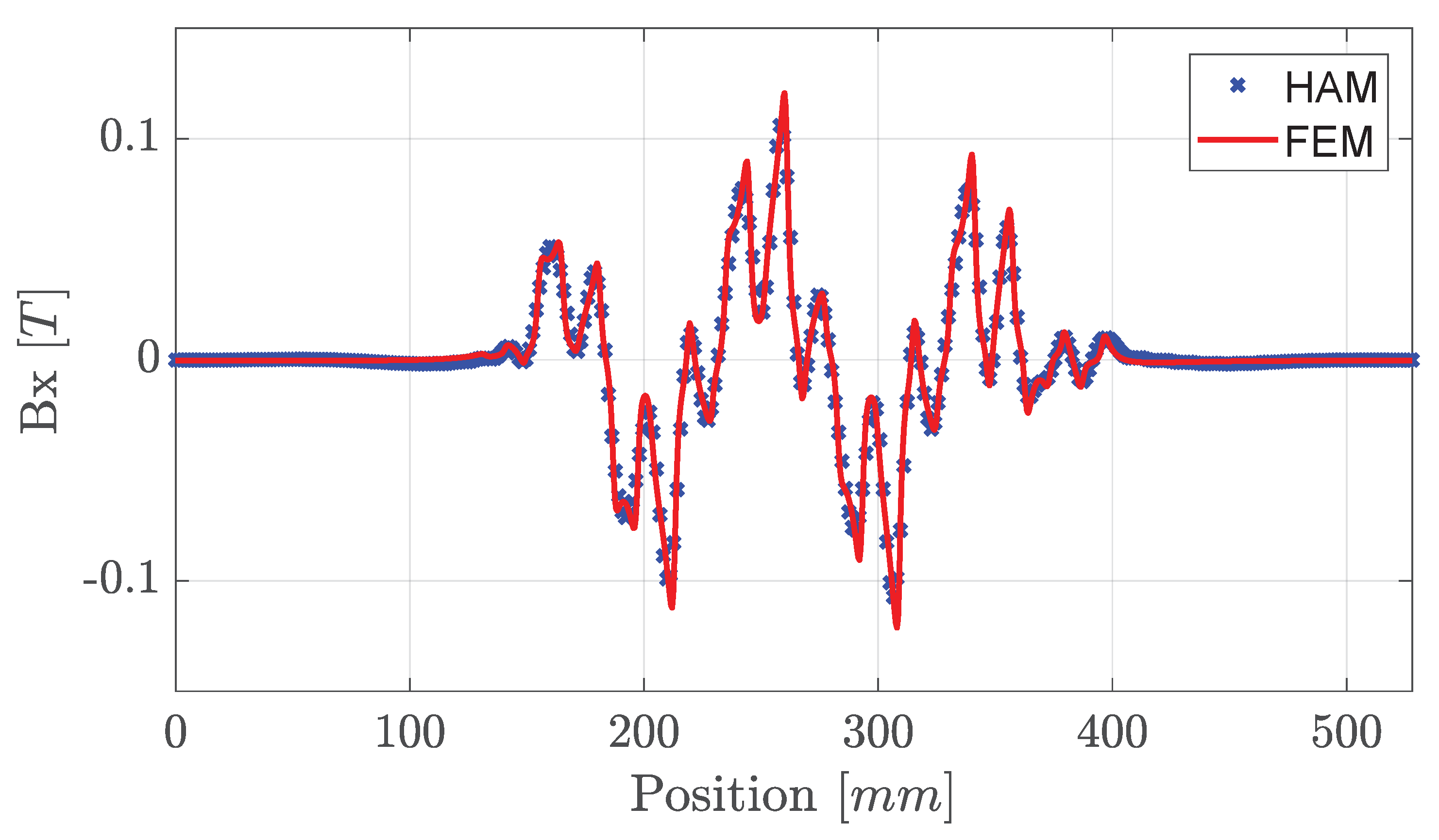
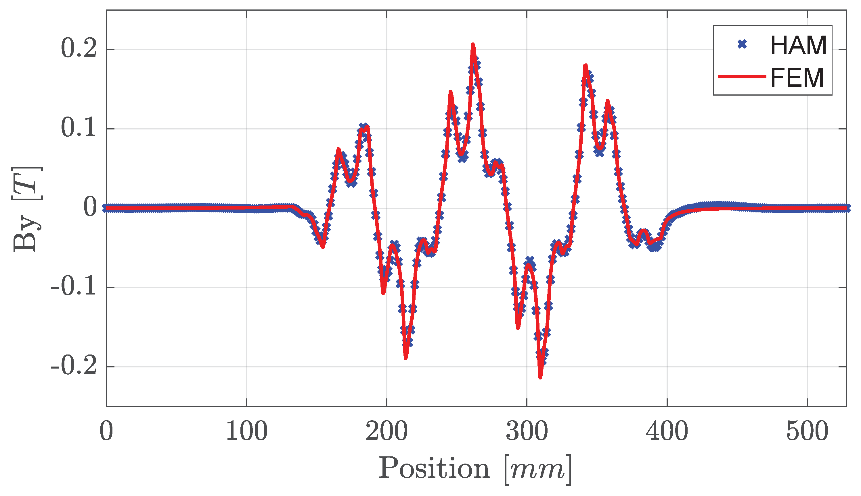
Considering velocity $v=0$ m/s, peak current $I_p=10$ A, and synchronous frequency $f=100$ Hz, the resulting magnetic flux density in the normal (Figure 6) and in longitudinal direction (Figure 7) was plotted against the steady-state FEA solution, showing excellent correspondence. The output thrust force, normal force, and Joule losses were calculated using (25)–(27), respectively, and predicted within 1.5%, 1.7%, and 3.1% when compared to FEA.

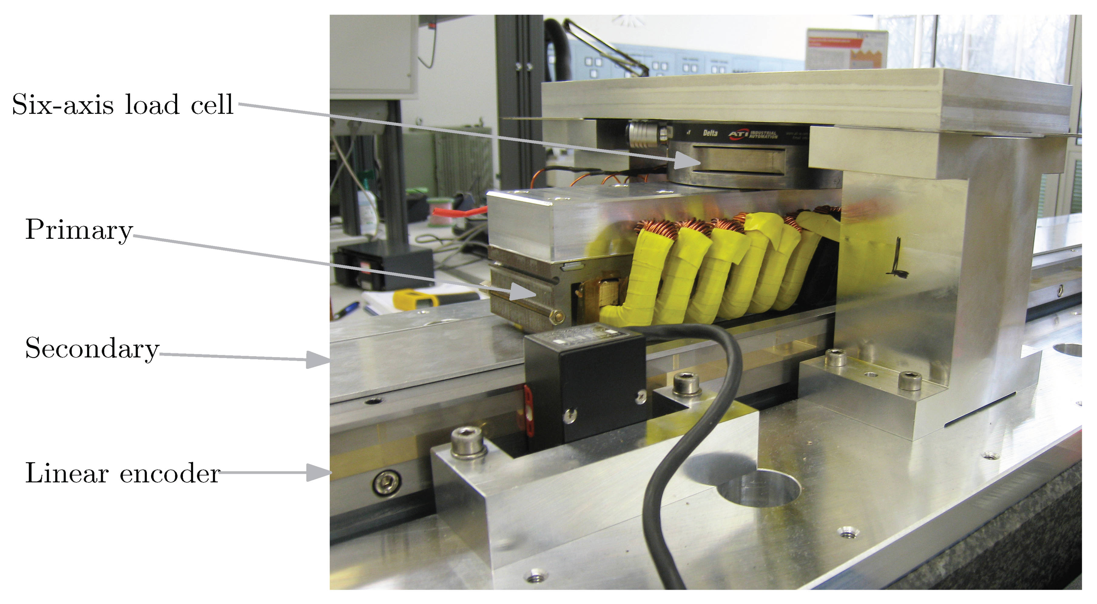
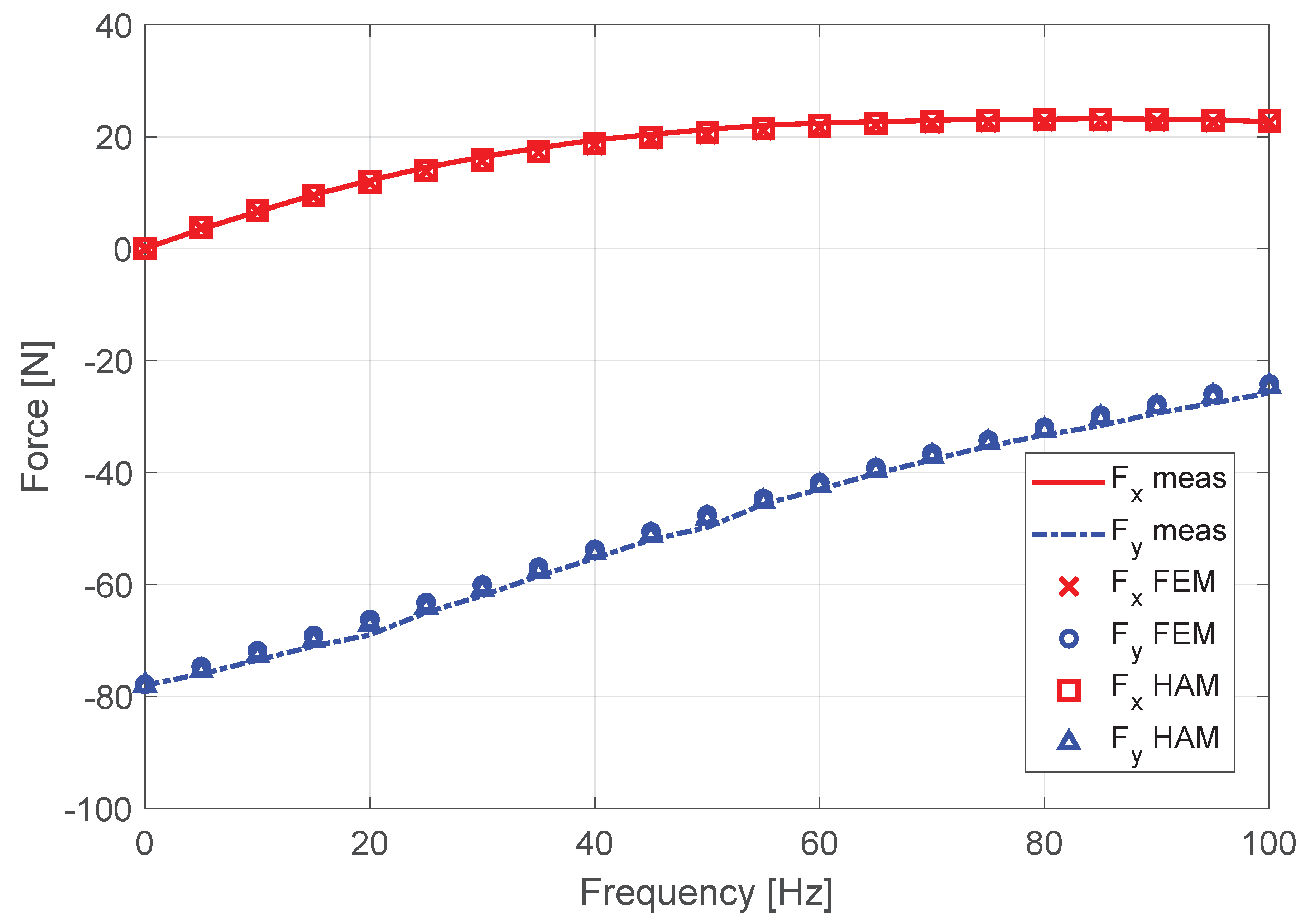
In addition, the thrust and normal forces, obtained at different synchronous frequencies from both the presented model and FEA, were validated by static measurements. As shown in Figure 8, the secondary of the LIM was mounted on a moving translator, while the mechanical construction on top of it held the primary and a six-axis load cell [14]. The thrust and normal force were measured with a fixed secondary and primary ($v=0$ m/s). For $I_p=10$ A, the results are shown in Figure 9.

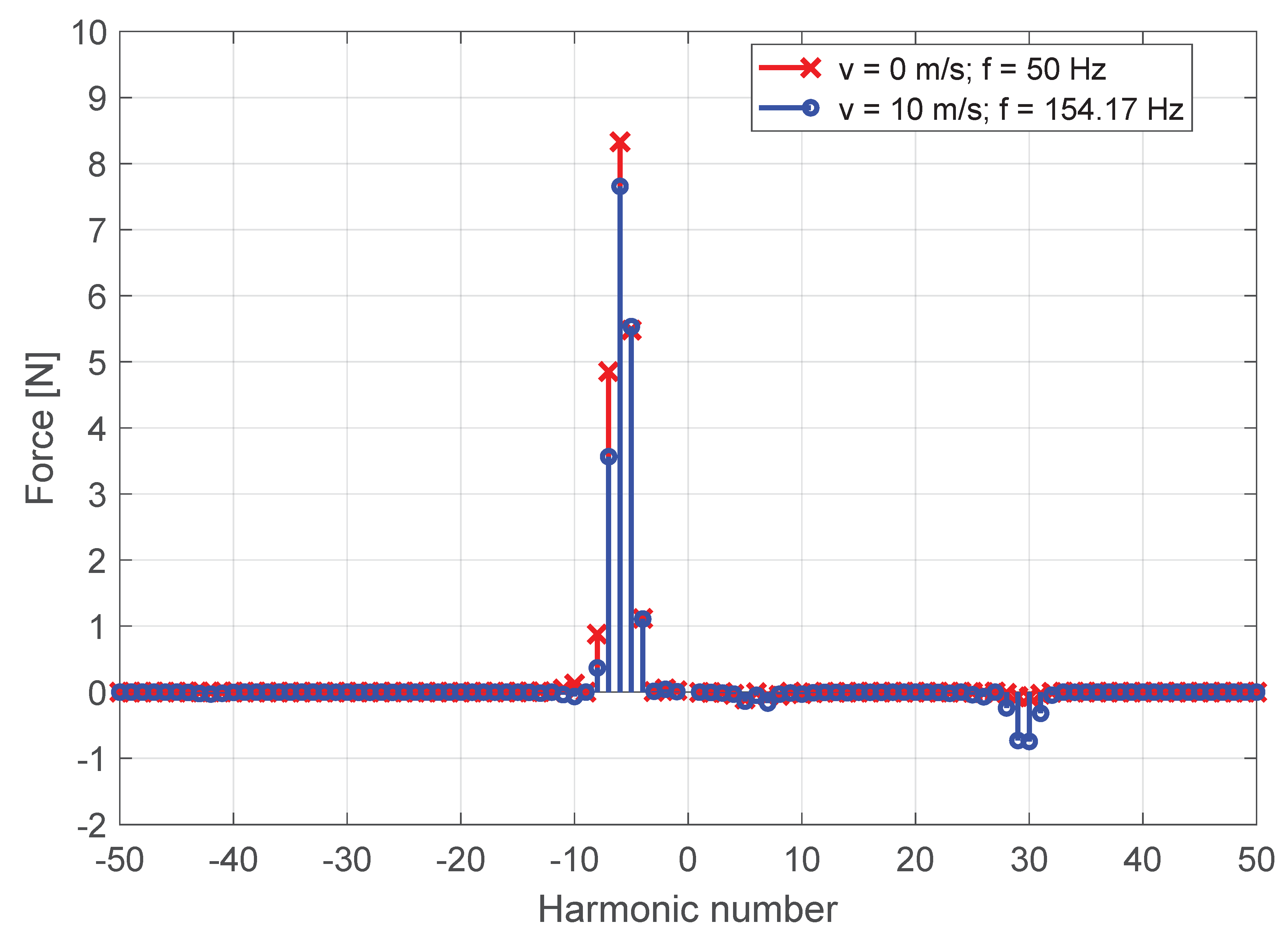
Having the resulting field represented by complex Fourier series allowed obtaining the contribution of each harmonic to the propulsion force. Including the end-effects of the primary provided information on the full harmonic spectrum contribution, as shown on Figure 10. As the velocity of the motor was accounted for in this steady-state hybrid model, two simulations at the same fundamental slip frequency:

$$\begin{array}{ccc}\hfill f_{slip}& =& f-\frac{v}{2{\tau }_1}\hfill \end{array}$$

(30)

were performed:

• Case 1: velocity $v=0$ m/s at frequency $f=50$ Hz,
• Case 2: velocity $v=10$ m/s at frequency $f=154.17$ Hz.

In Case 1, the eddy-currents generated in the static secondary were interacting with the traveling wave, produced by the three-phase primary winding, and thus, propulsion force in the positive x-direction was acting on the primary. The fundamental motor harmonic, contributing to the propulsion force generation, was defined by one periodical section of the primary. Due to the definition of this electromagnetic problem, where $x_p=12\tau$, the fundamental motor harmonic was equal to the sixth field harmonic in the Fourier series, and analogically, the fifth motor harmonic was equal to the thirtieth field harmonic in the Fourier series, as can be clearly seen in Figure 10. Additional thrust force contributions from the fifth and seventh field harmonics were caused by the end-effects, and the total thrust force in Case 1 was $F_x=20.4$ N.

As the velocity was accounted for in Case 2, new conductive material, unaffected by the induced magnetic field, was constantly seen by the front end of the primary, while there were still trailing eddy-currents in the conductive plate, behind the rear end of the motor. This effect caused the fifth motor harmonic (thirtieth field harmonic) to oppose the fundamental motor harmonic (sixth field harmonic), which was additionally reduced by the longitudinal end-effects, and thus, the generated thrust force was decreased to $F_x=15.8$ N, as seen in Figure 10.

4. Conclusions

In this paper, a 2D hybrid steady-state magnetic field model that included the full primary of a double-layer single-sided linear induction motor, thus accounting for the longitudinal end-effects, was presented. Compared to finite elements analysis, the model showed excellent correspondence of the magnetic field distribution inside the LIM. The velocity of the primary, with respect to the secondary, and the resulting longitudinal end-effects were accounted for in the solution of the magnetic field. The obtained thrust and normal forces for different fundamental slip frequencies had a discrepancy within 1.7% compared to FEA and were verified by static measurements. Future research will focus on derivation of secondary parameters and adding saturation effects to the model, which will allow the implementation for different motor topologies.